Article

Stochastic Analysis of the Marginal and Dependence Structure of Streamflows: From Fine-Scale Records to Multi-Centennial Paleoclimatic Reconstructions

by
Alonso Pizarro
1,
Panayiotis Dimitriadis
2,*,
Theano Iliopoulou
2,
Salvatore Manfreda
3 and
Demetris Koutsoyiannis
2
1
Escuela de Ingeniería en Obras Civiles, Universidad Diego Portales, Santiago 8370109, Chile
2
Department of Water Resources and Environmental Engineering, School of Civil Engineering, National Technical University of Athens, Heroon Polytechneiou 5, 15880 Zographou, Greece
3
Department of Civil, Architectural and Environmental Engineering, University of Naples Federico II, 80125 Naples, Italy
*
Author to whom correspondence should be addressed.
Hydrology 2022, 9(7), 126; https://doi.org/10.3390/hydrology9070126
Submission received: 12 May 2022 / Revised: 28 June 2022 / Accepted: 7 July 2022 / Published: 17 July 2022
(This article belongs to the Section Statistical Hydrology)

Abstract

:
The identification of the second-order dependence structure of streamflow has been one of the oldest challenges in hydrological sciences, dating back to the pioneering work of H.E Hurst on the Nile River. Since then, several large-scale studies have investigated the temporal structure of streamflow spanning from the hourly to the climatic scale, covering multiple orders of magni-tude. In this study, we expanded this range to almost eight orders of magnitude by analysing small-scale streamflow time series (in the order of minutes) from ground stations and large-scale streamflow time series (in the order of hundreds of years) acquired from paleocli-matic reconstructions. We aimed to determine the fractal behaviour and the long-range de-pendence behaviour of the streamflow. Additionally, we assessed the behaviour of the first four marginal moments of each time series to test whether they follow similar behaviours as sug-gested in other studies in the literature. The results provide evidence in identifying a common stochastic structure for the streamflow process, based on the Pareto–Burr–Feller marginal dis-tribution and a generalized Hurst–Kolmogorov (HK) dependence structure.

1. Introduction

Describing the stochastic properties of streamflows is essential for hydrological modelling and flood risk management. However, the lack of continuous and long streamflow records makes a proper characterization of the process in stochastic terms challenging. Technological advances have fostered the use of novel monitoring frameworks able to reduce costs. The HARMONIOUS COST Action provided a large ensemble of innovative practices, algorithms, and data assimilation techniques to enhance our ability to monitor rivers (see details in [1,2]). These target practices and methods could be further improved by incorporating the stochastic structure of streamflow (i.e., the marginal distribution and dependence functions). Such structures cannot be known a priori and are often estimated from single short time series (e.g., less than 30 years, which is considered the typical climatic scale). However, because the estimators of both the marginal and dependence structures rely on the selected model, it is argued that their values cannot be robustly estimated when the following conditions are met: (a) the process is characterized by long-range dependence (LRD; also called long-term persistence, long-term memory, Hurst phenomenon [3] or Hurst–Kolmogorov (HK) behaviour [4]), which is the dominant case, especially in the hydrological cycle processes (e.g., see global-scale analyses from reanalysis data in [5]; and in hydrometeorological stations in [6]); (b) a single and often short time series of a process is analysed (e.g., of some years of length or even smaller), which is a central practice in the literature; and, (c) statistical bias is not taken into account, which is also the most common practice (e.g., see the discussion on the importance of bias in [7,8]). The mentioned practices are considered unreliable because they may lead to severe underestimation of the expected values (depending on the strength of the LRD behaviour) and thus of the parameters of the selected models.
Natural processes are expected to exhibit specific stochastic similarities because they are all bounded by the law of entropy extremization (e.g., see the physical justification of the LRD in [9]). This concept has been confirmed in recent studies, such as the one by Dimitriadis et al. [6], where stochastic similarities (including LRD) are traced in all key hourly and daily-scale hydrological-cycle processes (i.e., surface air temperature, relative humidity, dew-point, close-to-surface wind speed, atmospheric pressure, streamflow, and precipitation) by analysing the most comprehensive available databases (i.e., including tens of billions of values from several thousands of globally distributed stations). Notably, it is illustrated that even though the stations are located in different climatic regimes, a pattern exists in the values of the marginal moments and the dependence structure when they are robustly estimated from data. Thus, it is argued that the impact of the climatic conditions is mainly mirrored by the different values of the marginal and dependence structure model parameters, leaving the distribution type and the dependence model structure almost unaltered after applying simple standardization techniques.
Thus, the aim of this study was to estimate the stochastic structure of the streamflow process over an extensive range of temporal scales, from fine scales (in the order of minutes) to very large timescales (in the order of hundreds of years). For this aim, we used several global databases of finer-scale streamflow time series and larger-scale paleoclimatic reconstructions, for which the scientific interest has grown (e.g., see discussions and methods in recent studies [10,11,12]) but without having performed any similar stochastic analysis. The stochastic dependence structure, and in particular, the importance of the LRD in hydrology and streamflow, has been highlighted in several studies analysing large-scale observational datasets [13,14,15,16,17,18,19,20,21,22,23,24]; however, the temporal coverage of these datasets is usually limited compared with those of paleoclimatic reconstructions. To the best of our knowledge, this is the first time that such an extensive range of temporal scales (spanning approximately eight orders of magnitude) has been assembled and studied for the streamflow process from both observational records and paleoclimatic reconstructions. This range of scales and data enables unique insights into the process’s stochastic properties. The analysis also applied the K-moments [8] for the estimation of the first four moments, which present some advantages compared with the most commonly used classical (raw or central) or L-moments [25] estimators.
Additionally, the second-order dependence structure is expressed herein through the climacogram (i.e., the variance of the averaged process at the scale domain [26]), which is adjusted for estimation bias as opposed to the commonly used estimators (see definitions in Beran [27], and comparison among other estimators in [6,7]). Finally, the resulting model form and parameters (such as the first four K-moments, and the fractal and Hurst parameters) are compared with those reported in other studies, where a higher number of streamflow stations was assessed. Notably, previously published studies used shorter lengths, a smaller range of scales, and lower resolution.
The manuscript is organized as follows: Section 2 presents the applied methodology focusing on the marginal and second-order dependence structure metrics; Section 3 contains the results; and Section 4, which precedes the conclusions, discusses their usefulness at operational and research levels.

2. Methodology

A common task in stochastic analyses is the estimation of the second-order dependence structure of a geophysical process from sample series of different scales (e.g., hourly, monthly, or annual). After performing a non-linear transformation in order to diminish the effect of double periodicity of the geophysical process on the dependence structure, this task becomes easy for a white-noise correlation structure (i.e., assumption of independent increments of the process) and by assuming a single distribution function, because it requires only to transform all samples to the largest scale among them, and then simply merge them as if they were drawn from a single sample of the process. However, in the presence of long-range dependence—a dominant attribute of geophysical processes—this task becomes challenging and cannot be accomplished with such naive procedures. The second-order dependence structure of a process from samples of different scales can be estimated more robustly through the variance (adjusted for bias) in the scale domain (where the variance of the averaged process vs. time scale is called the climacogram) rather than in other domains (e.g., lag of frequency). Following the proposed methods, we estimated streamflow’s fractal and long-range dependence behaviour more accurately, assuming they are not considerably affected by different climatic conditions. We combined records from sub-hourly scale resolution to paleoclimatic reconstructed time series with annual resolution. The estimated scales ranged from minutes to hundreds of years; thus, they were used to extend the range of streamflow scales used in literature.

2.1. Second-Order Dependence Structure Metrics

For the estimation of the LRD, the climacogram was applied, which is defined as [28]:
γ ( k ) : = var [ 0 k x _ ( y ) d y ] / k 2
where k is the scale in units of time.
For the estimation of the fractal behaviour, the so-called climacogram-based variogram (or climaco-variogram) was employed, which is simply defined as γ ( 1 ) γ ( k ) [28].
For the estimation of both the LRD and the fractal behaviours, the climacogram-based spectrum (CBS, or climacospectrum)) was used, defined as [28]:
ψ ( k ) : = k ( γ ( k ) γ ( 2 k ) ) ln 2
The estimator of variance for both the above metrics can be expressed as [8,29]:
γ ^ _ ( k ) = 1 n / κ i = 1 n / κ ( x _ i ( κ ) μ _ ^ ) 2
where κ = k / Δ is the dimensionless scale, Δ is the time resolution of each sample time series, n / κ is the integer part of n/κ, and x _ i ( κ ) is the ith element of the averaged sample of the process at scale κ, i.e.,
x _ i ( κ ) = 1 κ j = ( i 1 ) κ + 1 i κ x _ j
The statistical bias of the above estimator of the above second-order climacogram, γ ^ _ ( κ Δ ) at resolution Δ, can be expressed as [8,29]:
E [ γ ^ _ ( κ Δ ) ] = γ ( κ Δ ) γ ( n / κ κ Δ )
For convenience and for the identification of the fractal and Hurst parameter, the standardized climacogram and CBS are used, i.e., γ ^ _ ( k ) / γ ^ _ ( 1 ) and ψ ^ _ ( k ) / ψ ^ _ ( 1 ) , respectively, where γ ^ _ ( 1 ) and γ ^ _ ( 2 ) are the sample variances of finer-resolution time series.
Finally, for the appropriate selection of the climacogram model to assess the fractal behaviour and LRD of the streamflow process, we selected an expression that combines both behaviours, i.e., [28,29]:
γ ( k ) = λ ( 1 + ( k / a ) 2 M ) ( 1 H ) / M
where λ is the variance of the process, a is a scale parameter in units of the scale k, M is the dimensionless fractal parameter indicative of the roughness (M < 0.5) or smoothness (M > 0.5) of the fine scales (whereas the case M = 0.5 corresponds to the absence of fractal behaviour), and H is the Hurst parameter, indicative of the strength of the LRD (i.e., for 0.5 < H < 1, whereas the case H = 0.5 corresponds to a white-noise behaviour, and 0 < H < 0.5 to an anti-persistence behaviour ).

2.2. Marginal Structure Metrics

It has been shown that the high-order moments (i.e., skewness, kurtosis and beyond) indicate the process’s intermittence and tail behaviour [29]. However, the preservation of additional moments (beyond the fourth) can further contribute to the simulation of the marginal structure and joint probability distributions for the second-order statistics of demanding engineering applications (e.g., at hourly resolution [30]), such as streamflow [31]. Here, comparing the results of the global-scale analysis conducted by Dimitriadis et al. [6], we assessed the behaviour of the marginal structure of streamflow through the first four moments (i.e., mean, variance, skewness, and kurtosis) of the examined sample time series. Specifically, we applied the unbiased estimators of the standardized classical central (C-) moments, as well as the corresponding knowable (K-) moments, which are shown to be invariant, homogeneous and approximately unbiased even for high orders (as compared with the classical moments), and can incorporate the joint effect between the marginal and the second-order dependence structure of a process (as compared with the well-known L-moments; [10]), thus enabling more reliable estimations from data [8].
Here, we used a version of the K-moments, called hyper-central K-moments, which present several additional advantages in model fitting and inference from data, and are defined as (see definitions, discussion, and abundant applications in [8,32]):
K p q + : = ( p q + 1 ) E [ ( 2 F ( x _ ) 1 ) p q ( x _ μ ) q ]
for p q , where p and q reflect the order of the estimation, x is the stochastic process of interest with marginal probability distribution F ( x _ ) , and μ is the process mean.
The hyper-central moments, estimated from the central K-moments, are defined as:
K p q : = ( p q + 1 ) E [ ( F ( x _ ) ) p q ( x _ μ ) q ]
For example, the hyper-central K-skewness and K-kurtosis can be defined through the hyper- and central K-moments as:
S = K 32 + K 22 + = 2 K 32 K 22 2
and
K = K 42 + K 22 + = 4 K 42 K 22 6 K 32 K 22 + 3
The sample estimator of the central K-moments, approximately adjusted for bias, can be expressed as:
K ^ _ p 2 = n n 1 i = p n p 1 n Γ ( n p + 2 ) Γ ( n ) Γ ( i ) Γ ( i p + 2 ) ( x _ ( i : n ) μ _ ^ ) 2
where n is the length of the sample, μ _ ^ = i = 1 n x _ i / n is the estimator of the mean, and x _ ( i : n ) is the observed sample rearranged in ascending order.

2.3. Global-Scale Data Extraction and Processing

The analysed streamflow dataset included both measured and reconstructed data (paleoclimatic reconstructions) with high-quality and 0% missing values. The latter expanded the range of analysis by incorporating more information. Datasets are described in Table 1, where the number of monitoring stations and period of observation are presented. In addition, Figure 1 illustrates the differences among the examined time series.
The paleoclimatic reconstruction dataset has an annual temporal resolution encompassing 55 minimally regulated stations within the Missouri River catchment in the USA. The reconstruction relies on canonical correlation and tree-ring-based analyses [33], and in total, 533 years were retrieved following this methodology (access in: https://www.ncei.noaa.gov/access/paleo-search/study/19520, accessed on 10 May 2022). The catchment area ranges from around 4 to 13,000 km2.
The updated Sacramento time series reconstructs 1077 years (from 901 to 1977) based on tree-ring chronologies [34,35]. The reconstructed streamflow consists of four gauges: (i) Sacramento River at Bend Bridge; (ii) Feather River inflow to Lake Oroville; (iii) Yuba River at Smartville; and (iv) American River inflow to Folsom Lake (access in: https://www.ncei.noaa.gov/pub/data/paleo/treering/reconstructions/california/sacramento-flow-cdwr.txt, accessed on 10 May 2022).
The Swiss streamflow data were requested from the Federal Office for the Environment (FOEN; access in: https://www.bafu.admin.ch/bafu/en/home/topics/water.html, accessed on 10 May 2022). In total, 39 gauging stations were considered and filtered by minimizing anthropogenic effects and encompassing a wide range of catchment characteristics. Indeed, the streamflow is not altered by urban areas or regulated by lakes. The monitoring time ranges from 1974 to 2017 (with a minimum number of 20 years), and the catchment areas are small to medium-sized.

3. Results

The first four moments from both databases are depicted and compared in Figure 2 and Figure 3. The cloud data from the analysis performed in [6] (where over 10 million data values from over 1500 stations are assessed) are also plotted in Figure 2 and Figure 3, for comparison of the behaviour of different temporal scales (i.e., annual and 10 min scales vs. hourly and daily scales).
Specifically, the data cloud of the mean vs. the standard deviation is depicted in Figure 2, where the latter was estimated through the classical estimator. The information drawn from the joint behaviour of these two is of high scientific interest and can also be found useful at operational levels (e.g., in an engineering design), where usually only the mean value can be robustly estimated due to limited data. Similar interest is generated when observing the skewness and kurtosis, as shown in Figure 3. It is noted that in this figure, the classical estimators are used for the estimation of both statistical moments.
Additionally, both data clouds of the mean (μ) vs. the standard deviation (σ) and the skewness (s) vs. the kurtosis (k) coefficients can be well fitted by power-law functions, i.e., σ = 2.0 μ0.9 (R2 = 0.28 when including all values; and R2 = 0.87 when the reconstructed time series with the largest standard deviation value is omitted, which was causing a large residual value compared to the total sum of residuals between the model and data-values; see circled value in Figure 2), and k = 3.4 s1.7 (R2 = 0.97) when all values are included and k = 2.9 s1.8 (R2 = 0.97) when the 15 reconstructed time series with the smallest skewness values below 1.2 are omitted (see circled values in Figure 3).
The information drawn from the first two moments could be representative and sensitive to the river geometry (e.g., small/large rivers mainly generate low/high-magnitude streamflows) or catchment size (e.g., small/large catchment sizes tend to generate lower/higher streamflow coefficients of variation) or climatic conditions at the location of the recording station (e.g., low/high precipitation intensity may cause small/large variabilities, depending on the soil moisture and air humidity conditions). However, the information drawn from the skewness vs. kurtosis is indicative of the heaviness of the tail of the marginal structure of streamflow. For example, one may observe that several values of skewness and kurtosis of the paleoclimatic reconstructions are very low compared with the rest of the values and datasets. This is mainly caused by the fact that these time series are at an annual aggregation scale, which means that their tails are closer to Gaussianity.
Notably, classical moments beyond the second are unknowable, and their estimations can be misleading for small (or even extensive) time series lengths [8,32]. For a more robust analysis, one may implement the L-moments (see estimations in [6]). However, the latter do not consider the impact of the dependence structure, which in the case of a strong LRD behaviour is non-negligible. To acquire the latter effect, the so-called knowable (K-) moments were introduced by Koutsoyiannis [32]. Figure 4 shows them for the examined time series of all datasets. Similar power-law behaviour is observed, with a negligible difference between the 10 min discrete and the annual aggregated scale, between the K-skewness (S) and K-kurtosis (K), by omitting the 15 reconstructed time series with the smallest K-skewness below 0.6 (see circled values in Figure 4), i.e., K = 2.3 S0.3 (R2 = 0.90; the linear trendline, i.e., K = 0.6 S + 1.7, achieves a higher R2 = 0.93, but may not be considered physically consistent). Again, the aggregated reconstructed time series are expected to deviate from the rest of the data cloud and approach Gaussianity.
To estimate the second-order dependence structure through the variance vs. scale, we expressed all-time series to the smallest available scale of the data; here, it was the 10 min scale. Therefore, the time series from the paleoclimatic reconstructions, which are at an annual aggregated scale, are transformed into a 10 min scale by dividing each value of the climacogram of each time series by n2, where n = 365 × 24 × 6 is approximately the total number of 10 min in one year.
Subsequently, we constructed the climacograms, climaco-variograms and CBSs for all the time series of the Swiss stations and the paleoclimatic reconstructions, so that their expected values were estimated, adapting for bias, as explained in the previous section. Furthermore, all the above mean climacograms, climaco-variograms and CBSs were standardized (i.e., divided by their first value); for example, the mean climacograms for all scales and from both time series of the Swiss stations and the paleoclimatic reconstructions are divided by the average variance of their time series. Notably, only 90% of the available scales were depicted and used for model fitting, since estimations of variance from samples with fewer than 10 values are considered unreliable and misleading [7].
For illustration purposes, and in order to combine all the available scales from both sources (i.e., streamflow stations and paleoclimatic reconstructions), we adjusted the mean climacogram of the Swiss database to that of the paleoclimatic reconstructions at the annual scale (Figure 5 and Figure 6), by multiplying the latter with a coefficient so that both mean climacograms and mean climaco-variograms of the paleoclimatic reconstructions had equal values at the annual scale of the adapted for bias model.
Finally, for comparison of the LRD and fractal behaviours with the global-scale analysis in [6], we show the differences through the mean CBS (Figure 7) where, to focus only on these two behaviours, the adjustment between the Swiss and paleoclimatic datasets is employed at the model’s climatic scale. Interestingly, we observe that both analyses exhibit similar asymptotic behaviours. In fact, the differences between the fractal and Hurst parameters of the Swiss dataset (approximately M = 0.8 and H = 0.8) and the global-scale analysis of hourly resolution datasets (M = 0.78 and H = 0.78; [6]) are considered small.
Notably, for the fitting of Equation (6) at the climacogram and climaco-variogram, the scale parameter is estimated as a = 21 h. Additionally, the fitting of the model described in Equation (6) is considered adequate, with the exception of the intermediate drop in variance at the medium scales (see the difference when adjusting at the model’s climacogram and observed climacogram of the Swiss dataset), a phenomenon which is consistent with the rest of the literature (e.g., see discussion in [7] and results from the global-scale analysis in [6]). To capture this drop at the intermediate scales, a more sophisticated model is required, with additional parameters (see such examples in [7,8]).
As an overall observation of the results of the current analysis, the stochastic similarities are apparent in both the marginal (in terms of the first four moments) and the (second-order) dependence structure (in terms of the climacogram-based metrics). Practical implications of these and comparisons with those from the literature are further discussed in the next section.

4. Discussion

To estimate the strength of the LRD behaviour (known as the long-term persistence or Hurst phenomenon) of the streamflow process for scales related to engineering applications, we used time series based on paleoclimatic reconstructions with several hundreds of years of record lengths. The Hurst parameter was estimated approximately as H = 0.8 from the mean climacogram, which is indicative of a strong LRD behaviour (i.e., H >> 0.5). This is in agreement with the existent literature [3,5,6,31,36,37,38,39], where (a) the timeseries were recorded through stage–discharge measurements and not based on paleoclimatic reconstructions, (b) shorter lengths of time series were used to estimate the Hurst parameter, and (c) the selected estimators were either not adapted for bias, or not evaluated through the scale domain (but rather by the classical autocovariance-based metrics of the lag or frequency domains) or were based on the estimation of a single (or only a few) streamflow time series. An example of a practical application of the estimation of the LRD behaviour is when synthetic time series are required in areas where only short-length streamflow records are available. A typical misconception in stochastic hydrology is to provide synthetic time series that only preserve the statistical characteristics of an observed short-length sample. The LRD behaviour can affect all temporal scales; therefore, it is suggested that any prediction method [37,40,41] preserves the Hurst parameter evaluated from the current (or similar) analysis, and not the one estimated from shorter-length records.
For the fractal behaviour of the streamflow, records with a temporal resolution in the order of minutes were considered. The fractal parameter was estimated approximately as M = 0.8 from the mean climaco-variogram, which is consistent with the existing literature [6,31]. In fact, Vavoulogiannis et al. [31] estimated the fractal parameter from hourly-resolution timeseries as M = 0.72. All these results are indicative of a smooth behaviour (i.e., M > 0.5) rather than a rough behaviour (i.e., M < 0.5), which is the dominant rule for the rest key hydrological-cycle processes at hourly scale (i.e., precipitation, wind speed, air temperature, atmospheric pressure, humidity and dew-point) and turbulent processes [6,29]. It is also interesting to recall that in the global-scale analysis [6], the fractal behaviour of streamflow was characterized as slightly rough for the daily resolution datasets (i.e., M = 0.43 < 0.5), whereas for the hourly resolution time series, the fractal parameter was estimated as M = 0.78. The latter can be justified by the fact that for larger temporal scales, the fractal behaviour of a process is expected to be absent (i.e., M = 0.5) and to reveal its nature (i.e., smooth or rough) only at smaller scales.
An additionally interesting result of the current analysis is the similarities and agreement depicted among the first four marginal moments and the different datasets. Despite the different nature, climatic conditions and scale of the reconstructed time series, their marginal structure—as quantified through the mean and standard deviation as well as the skewness and kurtosis—is similar to the hourly and daily-scale analysis conducted by Dimitriadis et al. [6]. This result can be useful, for instance, in regionalization analyses or when it is not possible to robustly estimate one of the marginal moments from a sample. In the case of a short-length sample, the estimation uncertainty of the mean value may be found to be small, but that of the standard deviation can be larger. In such a scenario, one may use the suggested power-law expression to estimate the standard deviation based on the mean.
Moreover, the provided overall data cloud from all datasets can be used to perform a first empirical check of a new (short or long) time series and assess whether its sample moments fall into these data clouds. If its moment values do not fall into these data clouds, it does not necessarily mean that the data are erroneous, although it could be an indication that more careful analyses are required.
Additionally, because the new data analysed in this work also fell into the data cloud of the first four marginal moments, it was concluded that the Pareto–Burr–Feller probability distribution function can also be selected as a potential candidate for fitting, following the same stochastic hierarchy among the other key hydrological-cycle processes (as described in [6]). An important remark is that when LRD is present and explicitly preserved, the first four moments can capture a vast range of scales of a synthetic time series (see discussion, algorithms and applications in [28,29]). Additionally, in an analysis of any range of scales or related to extremes, more moments may need to be preserved (see discussion, algorithms and applications in [8,30,42]), or even additional attributes related to streamflow [43].
Finally, it is useful to note that the values within the data cloud of the skewness–kurtosis estimated from the K-moments (see Figure 4) form a single cluster (which can be accurately described by a power-law function), whether the skewness–kurtosis data cloud estimated from the central moments (see Figure 3) presents two power-law-type behaviours (i.e., one for small skewness records and one for larger records). By closely observing the lowest skewness–kurtosis value in Figure 3, we see that it originated from the Sacramento paleoclimatic reconstruction, which consists of 1077 values, whereas the other reconstructions consist of more than 500 values. However, the estimation of skewness and kurtosis through the K-moments for the specific reconstructed time series is not separated from the rest values of the data cloud. This can be justified by the fact that the K-moments present more advantages than central (or raw or even L, and other types of) moments, resulting in more robust estimations, even in longer records and in processes that exhibit LRD behaviour (see extended analysis and examples in the studies by Koutsoyiannis [8,32], while the L-skewness vs. L-kurtosis graph for the global-scale analysis can be viewed in [6]).
An additional useful remark from this study is that one may argue that if additional records will be available in the future with longer lengths or finer resolutions, then a re-evaluation of the Hurst and fractal parameters, respectively, would be possible. Although this is true (and we should always highlight the need for additional, finer resolution and longer records), the current analysis can set a foundation for studies related to flood management, where even for flash floods and for the larger return period of 1000 years, the results of the current analysis can be assumed adequate for a risk assessment. The latter can also be used to infer flood variability from fine temporal scales (e.g., minute, hourly and daily) to multi-centennial temporal scales.

5. Conclusions

Streamflow time series (from observational records and paleoclimatic reconstructions, forming a unique range of temporal scales of the order of minutes to hundreds of years) were analysed to determine the stochastic properties of the process. Results showed that the streamflow process is smooth at small scales, i.e., characterized, on average, by a fractal parameter of M = 0.8, and strongly persistent at large scales, i.e., characterized by long-range dependence with a parameter H = 0.8. Furthermore, the first four statistical moments (estimated from classic and K-moments) determine a useful relationship for operational and scientific practices. In particular, it was found that a power-law function can fit observations following a common stochastic behaviour. The latter leads to concluding that the Pareto–Burr–Feller probability distribution function, which is found to be a good candidate distribution for various hydrological-cycle processes in the literature, can also describe well these streamflow datasets.
Overall, these results complement previous studies on the stochastic structure of streamflow by significantly extending the empirical evidence from minute to centennial scales. They strengthen the hypothesis that the multi-scale streamflow process can generally be characterized by a Pareto–Burr–Feller marginal distribution and an HK-type dependence model, with the specific parameters determined by the local hydrometeorological processes and geophysical conditions. The identified common stochastic structure can be useful to support estimation at sites with limited data and serve as a basis for streamflow regionalization analyses. Furthermore, this study paves the way for the construction of a stochastic model for streamflow based on a common structure validated on a global spatial scale and a temporal scale ranging from minutes to centuries.

Author Contributions

Conceptualization, A.P., P.D., T.I., S.M. and D.K.; methodology, A.P., P.D., T.I., S.M. and D.K.; formal analysis, A.P., T.I. and P.D.; writing—original draft preparation, A.P. and P.D.; writing—review and editing, A.P., P.D., T.I., S.M. and D.K.; visualization, A.P., T.I. and P.D.; supervision, S.M. and D.K.; funding acquisition, S.M. and D.K. All authors have read and agreed to the published version of the manuscript.

Funding

This research was carried out/funded in the context of the project “Development of Stochastic Methods for Extremes (ASMA): identification and simulation of dependence structures of extreme hydrological events” (MIS 5049175) under the call for proposals “Researchers’ support with an emphasis on young researchers—2nd Cycle”. The project was co-financed by Greece and the European Union (European Social Fund; ESF) by the Operational Programme Human Resources Development, Education, and Lifelong Learning 2014–2020. Hydrology 09 00126 i001 This research was also supported by the COST Action CA16219, “HARMONIOUS-Harmonization of UAS techniques for agricultural and natural ecosystems monitoring”.

Data Availability Statement

Data used in this paper can be found at the following websites: (a) https://www.ncei.noaa.gov/access/paleo-search/study/19520, accessed on 10 May 2022; (b) https://www.ncei.noaa.gov/pub/data/paleo/treering/reconstructions/california/sacramento-flow-cdwr.txt, accessed on 10 May 2022; (c) https://www.bafu.admin.ch/bafu/en/home/topics/water.html, accessed on 10 May 2022.

Conflicts of Interest

The authors declare no conflict of interest.

References

  1. Manfreda, S.; McCabe, M.F.; Miller, P.E.; Lucas, R.; Pajuelo Madrigal, V.; Mallinis, G.; Ben Dor, E.; Helman, D.; Estes, L.; Ciraolo, G.; et al. On the Use of Unmanned Aerial Systems for Environmental Monitoring. Remote Sens. 2018, 10, 641. [Google Scholar] [CrossRef] [Green Version]
  2. Perks, M.T.; Dal Sasso, S.F.; Hauet, A.; Jamieson, E.; Le Coz, J.; Pearce, S.; Peña-Haro, S.; Pizarro, A.; Strelnikova, D.; Tauro, F.; et al. Towards harmonisation of image velocimetry techniques for river surface velocity observations. Earth Syst. Sci. Data 2020, 12, 1545–1559. [Google Scholar] [CrossRef]
  3. Hurst, H.E. Long-Term Storage Capacity of Reservoirs. Trans. Am. Soc. Civ. Eng. 1951, 116, 770–799. [Google Scholar] [CrossRef]
  4. Koutsoyiannis, D. Hurst-Kolmogorov dynamics and uncertainty. J. Am. Water Resour. Assoc. 2011, 47, 481–495. [Google Scholar] [CrossRef]
  5. Koutsoyiannis, D. Revisiting the global hydrological cycle: Is it intensifying? Hydrol. Earth Syst. Sci. 2020, 24, 3899–3932. [Google Scholar] [CrossRef]
  6. Dimitriadis, P.; Koutsoyiannis, D.; Iliopoulou, T.; Papanicolaou, P. A Global-Scale Investigation of Stochastic Similarities in Marginal Distribution and Dependence Structure of Key Hydrological-Cycle Processes. Hydrology 2021, 8, 59. [Google Scholar] [CrossRef]
  7. Dimitriadis, P.; Koutsoyiannis, D. Climacogram versus autocovariance and power spectrum in stochastic modelling for Markovian and Hurst–Kolmogorov processes. Stoch. Environ. Res. Risk Assess. 2015, 29, 1649–1669. [Google Scholar] [CrossRef]
  8. Koutsoyiannis, D. Stochastics of Hydroclimatic Extremes—A Cool Look at Risk; Kallipos: Athens, Greece, 2021; 333p, ISBN 978-618-85370-0-2. Available online: https://repository.kallipos.gr/handle/11419/6522 (accessed on 1 April 2022).
  9. Koutsoyiannis, D. Hurst-Kolmogorov dynamics as a result of extremal entropy production. Phys. A 2011, 390, 1424–1432. [Google Scholar] [CrossRef]
  10. Ljungqvist, F.C.; Piermattei, A.; Seim, A.; Krusic, P.J.; Büntgen, U.; He, M.; Kirdyanov, A.V.; Luterbacher, J.; Schneider, L.; Seftigen, K.; et al. Ranking of tree-ring based hydroclimate reconstructionsof the past millennium. Quat. Sci. Rev. 2020, 230, 106074. [Google Scholar] [CrossRef]
  11. Nasreen, S.; Součková, M.; Vargas Godoy, M.R.; Singh, U.; Markonis, Y.; Kumar, R.; Rakovec, O.; Hanel, M. A 500-year runoff reconstruction for European catchments. Earth Syst. Sci. Data Discuss. 2021. [Google Scholar]
  12. Formetta, G.; Tootle, G.; Bertoldi, G. Streamflow Reconstructions Using Tree-Ring Based Paleo Proxies for the Upper Adige River Basin (Italy). Hydrology 2022, 9, 8. [Google Scholar] [CrossRef]
  13. Cox, D.R. Long-Range Dependence: A review, Statistics: An Appraisal. In Proceedings of the 50th Anniversary Conference, Bridlington, UK, 1–2 June 1984; David, H.A., David, H.T., Eds.; Iowa State University Press: Ames, IA, USA, 1984; pp. 55–74. [Google Scholar]
  14. Bloschl, G.; Sivapalan, M. Scale issues in hydrological modelling: A review. In Scale Issues in Hydrological Modelling; Kalma, J.D., Sivapalan, M., Eds.; John Wiley: New York, NY, USA, 1995; pp. 9–48. [Google Scholar]
  15. Cohn, T.A.; Lins, H.F. Nature’s style—Naturally trendy. Geophys. Res. Lett. 2005, 32. [Google Scholar] [CrossRef] [Green Version]
  16. Mudelsee, M. Long memory of rivers from spatial aggregation. Water Resour. Res. 2007, 43. [Google Scholar] [CrossRef]
  17. Hirpa, F.A.; Gebremichael, M.; Over, T.M. River flow fluctuation analysis: Effect of watershed area. Water Resour. Res. 2010, 46, 12. [Google Scholar] [CrossRef] [Green Version]
  18. Gudmundsson, L.; Tallaksen, L.M.; Stahl, K.; Fleig, A.K. Low-frequency variability of European runoff. Hydrol. Earth Syst. Sci. 2011, 15, 2853–2869. [Google Scholar] [CrossRef] [Green Version]
  19. Zhang, Q.; Zhou, Y.; Singh, V.P.; Chen, X. The influence of dam and lakes on the Yangtze River streamflow: Long-range correlation and complexity analyses. Hydrol. Process. 2012, 26, 436–444. [Google Scholar] [CrossRef]
  20. O’Connell, P.; Koutsoyiannis, D.; Lins, H.F.; Markonis, Y.; Montanari, A.; Cohn, T. The scientific legacy of Harold Edwin Hurst (1880–1978). Hydrol. Sci. J. 2016, 61, 1571–1590. [Google Scholar] [CrossRef] [Green Version]
  21. Serinaldi, F.; Kilsby, C.G. Irreversibility and complex network behavior of stream flow fluctuations. Phys. A Stat. Mech. Appl. 2016, 450, 585–600. [Google Scholar] [CrossRef] [Green Version]
  22. Graves, T.; Gramacy, R.; Watkins, N.; Franzke, C. A Brief History of Long Memory: Hurst, Mandelbrot and the Road to ARFIMA, 1951–1980. Entropy 2017, 19, 437. [Google Scholar] [CrossRef] [Green Version]
  23. Iliopoulou, T.; Aguilar, C.; Arheimer, B.; Bermúdez, M.; Bezak, N.; Ficchì, A.; Koutsoyiannis, D.; Parajka, J.; Polo, M.J.; Thirel, G.; et al. A large sample analysis of European rivers on seasonal river flow correlation and its physical drivers. Hydrol. Earth Syst. Sci. 2019, 23, 73–91. [Google Scholar] [CrossRef] [Green Version]
  24. Dimitriadis, P.; Iliopoulou, T.; Sargentis, G.-F.; Koutsoyiannis, D. Spatial Hurst–Kolmogorov Clustering. Encyclopedia 2021, 1, 1010–1025. [Google Scholar] [CrossRef]
  25. Hosking, J.R.M. L-Moments: Analysis and Estimation of Distributions Using Linear Combinations of Order Statistics. J. R. Stat. Soc. Ser. B Stat. Methodol. 1990, 52, 105–124. [Google Scholar] [CrossRef]
  26. Koutsoyiannis, D. HESS opinions, A random walk on water. Hydrol. Earth Syst. Sci. 2010, 14, 585–601. [Google Scholar] [CrossRef] [Green Version]
  27. Beran, J. Statistical Methods for Data with Long-Range Dependence. Stat. Sci. 1992, 7, 404–416. [Google Scholar]
  28. Koutsoyiannis, D. Generic and parsimonious stochastic modelling for hydrology and beyond. Hydrol. Sci. J. 2016, 61, 225–244. [Google Scholar] [CrossRef]
  29. Dimitriadis, P.; Koutsoyiannis, D. Stochastic synthesis approximating any process dependence and distribution. Stoch. Environ. Res. Risk A 2018, 32, 1493–1515. [Google Scholar] [CrossRef]
  30. Koutsoyiannis, D.; Dimitriadis, P. Towards generic simulation for demanding stochastic processes. Science 2021, 3, 34. [Google Scholar] [CrossRef]
  31. Vavoulogiannis, S.; Iliopoulou, T.; Dimitriadis, P.; Koutsoyiannis, D. Multi-scale temporal irreversibility of streamflow and its stochastic modelling. Hydrology 2021, 8, 63. [Google Scholar] [CrossRef]
  32. Koutsoyiannis, D. Knowable moments for high-order stochastic characterization and modelling of hydrological processes. Hydrol. Sci. J. 2019, 64, 19–33. [Google Scholar] [CrossRef] [Green Version]
  33. Ho, M.; Lall, U.; Cook, E.R. Can a paleo-drought record be used to reconstruct streamflow? A case-study for the Missouri River Basin. Water Resour. Res. 2016, 52, 5195–5212. [Google Scholar] [CrossRef] [Green Version]
  34. Meko, D.M.; Therrell, M.D.; Baisan, C.H.; Hughes, M.K. Sacramento River flow reconstructed to A. D. 869 from tree rings. J. Am. Water Resour. Assoc. 2001, 37, 1029–1040. [Google Scholar] [CrossRef]
  35. Meko, D.M. Sacramento River Annual Flow Reconstruction. International Tree-Ring Data Bank. IGBP PAGES/World Data Center for Paleoclimatology Data Contribution Series #2006-105; NOAA/NGDC Paleoclimatology Program: Boulder, CO, USA, 2006. [Google Scholar]
  36. Vogel, R.M.; Tsai, Y.; Limbrunner, J.F. The regional persistence and variability of annual streamflow in the United States. Water Resour. Res. 1998, 34, 3445–3459. [Google Scholar] [CrossRef] [Green Version]
  37. Koutsoyiannis, D.; Yao, H.; Georgakakos, A. Medium-range flow prediction for the Nile: A comparison of stochastic and deterministic methods. Hydrol. Sci. J. 2008, 53, 142–164. [Google Scholar] [CrossRef]
  38. Szolgayová, E.; Laaha, G.; Blöschl, G.; Bucher, C. Factors influencing long range dependence in streamflow of European rivers. Hydrol. Process. 2013, 28, 1573–1586. [Google Scholar] [CrossRef]
  39. Markonis, Y.Y.; Moustakis, C.; Nasika, P.; Sychova, P.; Dimitriadis, M.; Hanel, P.; Máca; Papalexiou, S.M. Global estimation of long-term persistence in annual river runoff. Adv. Water Resour. 2018, 113, 1–12. [Google Scholar] [CrossRef]
  40. Dimitriadis, P.; Koutsoyiannis, D.; Tzouka, K. Predictability in dice motion: How does it differ from hydrometeorological processes? Hydrol. Sci. J. 2016, 61, 1611–1622. [Google Scholar] [CrossRef] [Green Version]
  41. Papacharalampous, G.; Tyralis, H.; Pechlivanidis, I.G.; Grimaldi, S.; Volpi, E. Massive feature extraction for explaining and foretelling hydroclimatic time series forecastability at the global scale. Geosci. Front. 2022, 13, 101349. [Google Scholar] [CrossRef]
  42. Iliopoulou, T.; Koutsoyiannis, D. Revealing hidden persistence in maximum rainfall records. Hydrol. Sci. J. 2019, 64, 1673–1689. [Google Scholar] [CrossRef]
  43. Koutsoyiannis, D. Simple stochastic simulation of time irreversible and reversible processes. Hydrol. Sci. J. 2020, 65, 536–551. [Google Scholar] [CrossRef]
Figure 1. The reconstructed streamflow time series at Sacramento from 901 to 1977 (in 10× hm3/year and of annual resolution), the reconstructed streamflow time series from the Missouri database from 1473 to 2005 (with ID 6278300, in 10−2× hm3/year and of annual resolution) and the 6th streamflow recorded time series from the Swiss database ranging from 1974 to 2017 (in hm3/year and of aggregated monthly resolution).
Hydrology 09 00126 g001
Figure 2. Mean vs. standard deviation of streamflow time series from the analysis by Dimitriadis et al. [6] (daily and hourly time series, denoted as Global), for the Swiss dataset (10 min resolution, denoted as Swiss) and for the paleoclimatic reconstructions (annual time series, denoted as Paleo. Rec.).
Hydrology 09 00126 g002
Figure 3. Skewness coefficient vs. kurtosis coefficient of the streamflow time series from the Dimitriadis et al. [6] analysis (daily and hourly time series, denoted as Global), for the Swiss dataset (10 min resolution, denoted as Swiss) and for the paleoclimatic reconstructions (annual time series, denoted as Paleo. Rec.).
Hydrology 09 00126 g003
Figure 4. K-skewness vs. K-kurtosis of streamflow time series from the analysis by Dimitriadis et al. [6] (daily and hourly resolution, denoted as Global), for the Swiss dataset (10 min resolution, denoted as Swiss), and for the paleoclimatic reconstructions (annual resolution, denoted as Paleo. Rec.).
Hydrology 09 00126 g004
Figure 5. The mean standardized climacogram for the analysis by Dimitriadis et al. [6] (daily and hourly resolution), for the Swiss dataset (10 min resolution) and for the paleoclimatic reconstructions (annual resolution).
Hydrology 09 00126 g005
Figure 6. The mean standardized climaco-variogram for the analysis by Dimitriadis et al. [6] (daily and hourly resolution), for the Swiss dataset (10 min resolution) and for the paleoclimatic reconstructions (annual resolution).
Hydrology 09 00126 g006
Figure 7. The mean standardized CBS for the analysis by Dimitriadis et al. [6] (daily and hourly resolution), for the Swiss dataset (10 min resolution) and for the paleoclimatic reconstructions (annual resolution).
Hydrology 09 00126 g007
Table 1. Summary of used datasets for the stochastic analysis.
Number of StationsTemporal ResolutionTotal Record Values/StationTime PeriodLocationTypeDatabase
Swiss dataset3910 min2.3 × 1061974–2017SwitzerlandStationsHyperlink
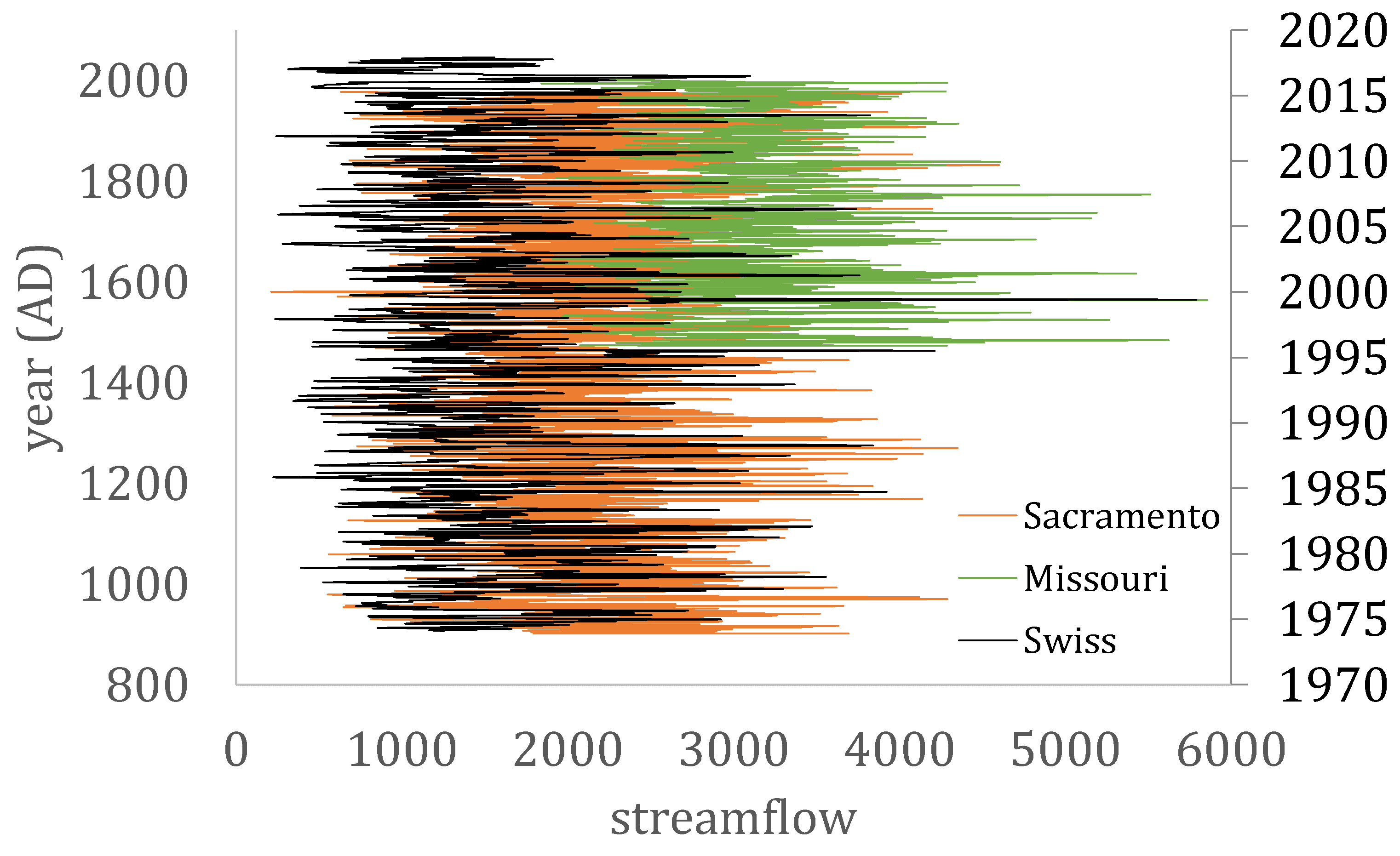
Missouri paleoclimatic reconstruction dataset55Annual5331473–2005Missouri river basin, USAReconstructionsHyperlink
Sacramento reconstruction timeseries1Annual1077901–1977Sacramento River, USAReconstructionHyperlink
Publisher’s Note: MDPI stays neutral with regard to jurisdictional claims in published maps and institutional affiliations.

