
On the Accuracy of Particle Image Velocimetry with Citizen Videos—Five Typical Case Studies


Abstract
:1. Introduction
2. Materials and Methods
2.1. Fudaa-LSPIV
- The area size (px). This is the size in pixels of the IA side (IA is square).
- S1, S2, S3, and S4 (px). These are the maximum displacements, in pixels, along the four directions of the IA up to which the normalized correlation is calculated.
- The minimum and maximum velocity threshold (m s−1). These values define the upper and lower limit of the range of the acceptable estimated velocity magnitudes. Non-acceptable values are filtered out.
- The minimum and maximum Vx threshold (m s−1). These values define the upper and lower limit of the range of the acceptable x-components of the estimated velocities.
- The minimum and maximum Vy threshold (m s−1). These values define the upper and lower limit of the range of the acceptable y-components of the estimated velocities.
- The minimum and maximum correlation. These values define the upper and lower limit of the normalized correlation values for a displacement to be considered acceptable.
2.2. Free-LSPIV
- The IA size (px × px). These are the sizes in pixels of the IA sides (IA is rectangle in Free-LSPIV, whereas it is square in Fudaa-LSPIV).
- The SA size (px × px). These are the sizes in pixels of the search area sides. SA defines the boundary within which the IA is displaced at each subsequent frame to calculate the correlation coefficient. The maximum correlation coefficient obtained corresponds to the most probable features’ displacement between the sequential frames. This is equivalent to S1, S2, S3, and S4 of Fudaa-LSPIV.
- The maximum velocity threshold (m s−1), the same parameter used in Fudaa-LSPIV.
- The minimum and maximum Vx threshold (m s−1), the same parameters used in Fudaa-LSPIV.
- The minimum and maximum Vy threshold (m s−1), the same parameters used in Fudaa-LSPIV.
- The minimum correlation coefficient, the same parameter used in Fudaa-LSPIV.
- The contrast adjustment parameter. This parameter controls the intensity capping [20], which is applied on the IA and SA before calculating the correlation. This is an additional feature of Free-LSPIV.
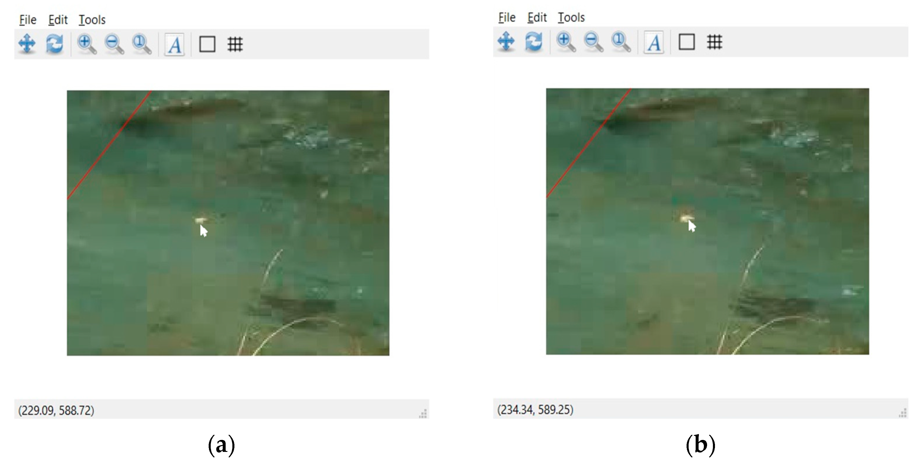
2.3. Manual Method
- Obtain the row and column of the feature in the initial frame i (let us say ri and ci) and the subsequent frame i + 1 (let us say ri+1 and ci+1). Figure 1 demonstrates how this is accomplished. According to this figure, the row and column pairs in the initial and subsequent frames are (229, 589) and (234, 589), respectively.
- Transform the row and column pairs to (x, y) pairs, employing a projective transformation [22], i.e., T(ri, ci) → (xi, yi) and T(ri+1, ci+1) → (xi+1, yi+1).
- If Δt is the time interval between frames i and i + 1, then the surface velocity can be estimated with the following formula:
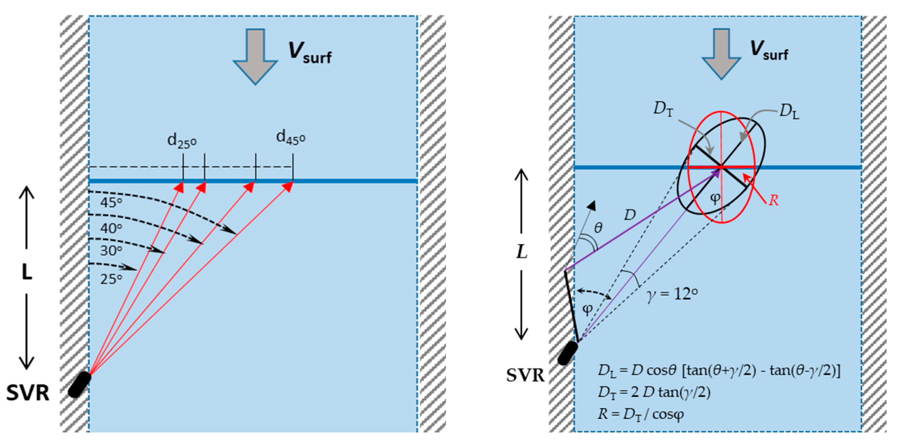
2.4. SVR Measurements
2.5. Case Studies
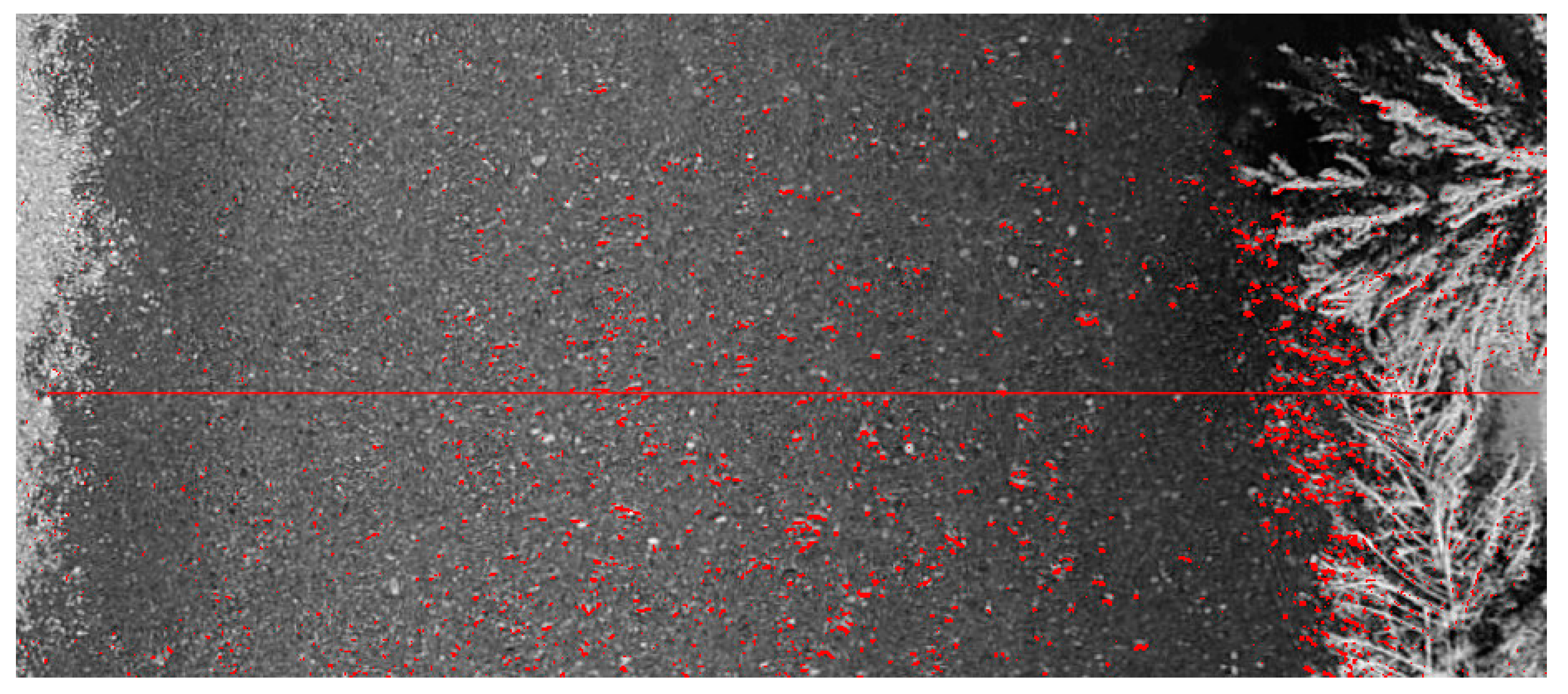
2.5.1. Case Study—Kolubara River
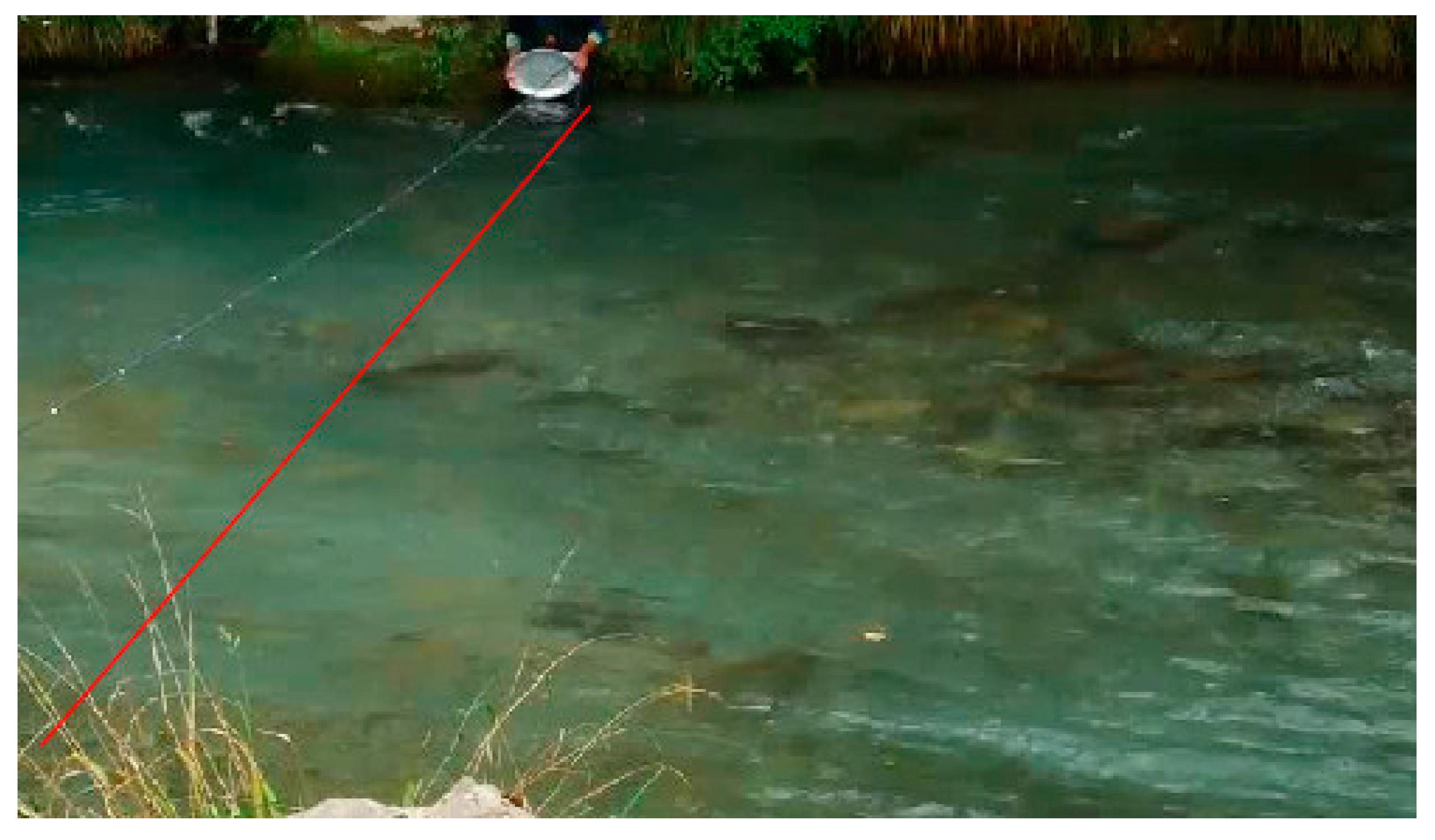
2.5.2. Case Study—Murg River
2.5.3. Case Study—Salmon River
2.5.4. Case Study—Loussios River at Atsicholos Bridge
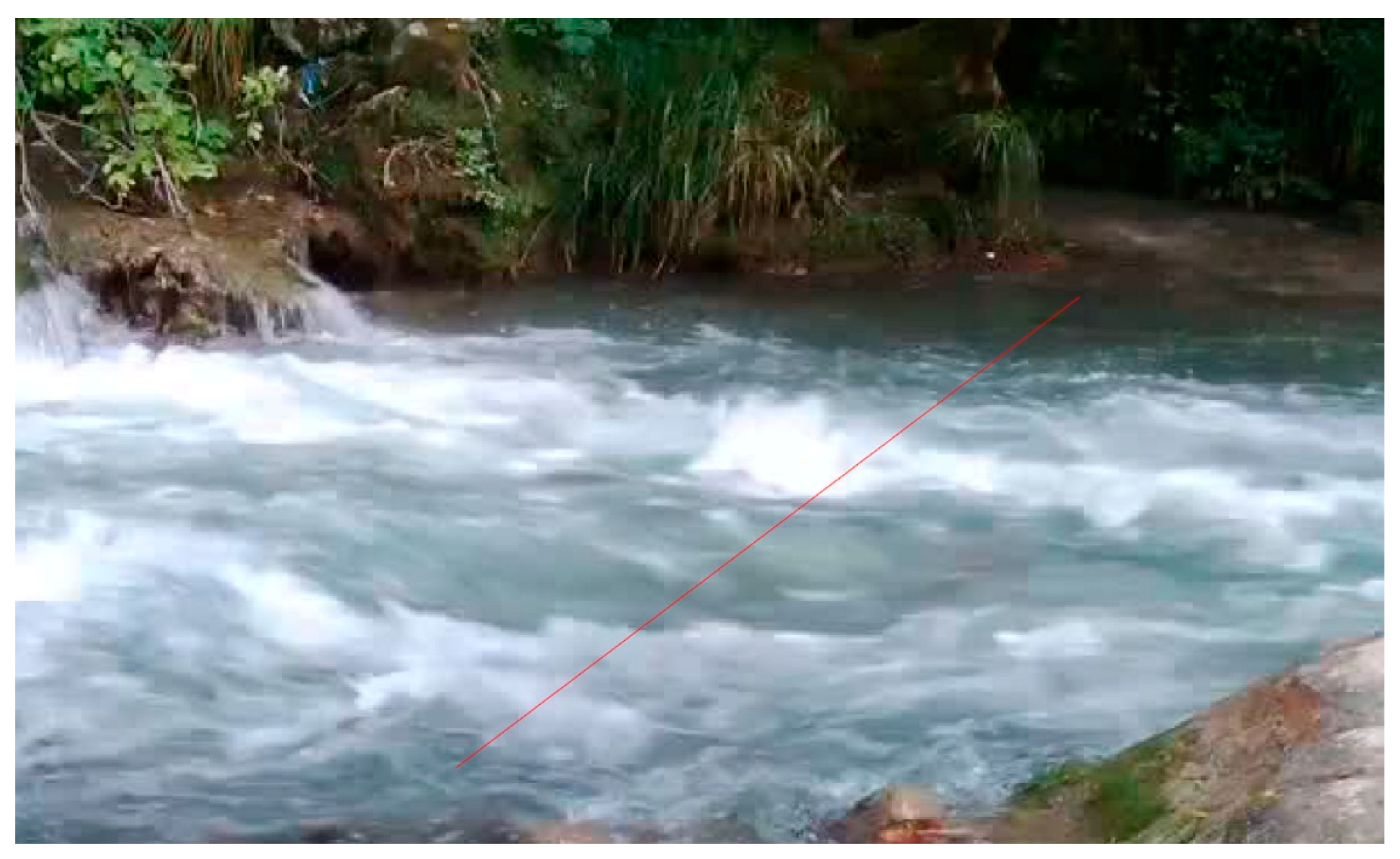
2.5.5. Case Study—Loussios River Upstream Atsicholos Bridge
3. Results
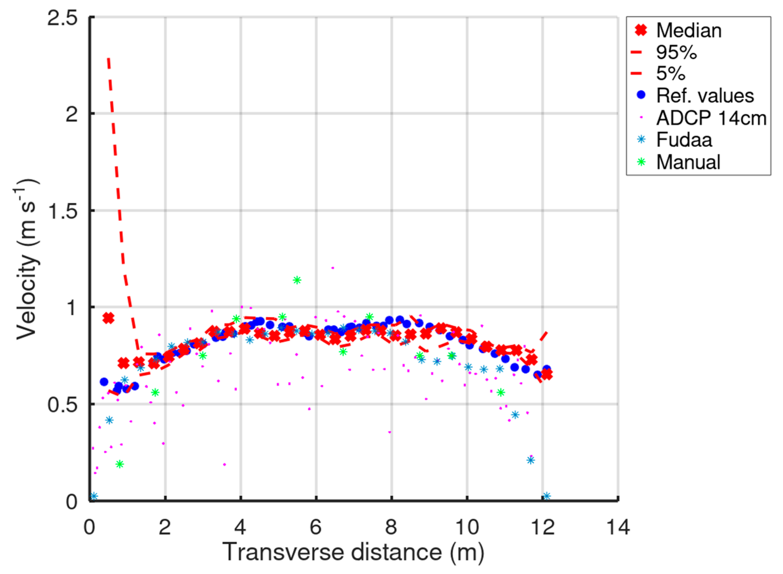
3.1. Kolubara River
3.2. Murg River
3.3. Salmon River
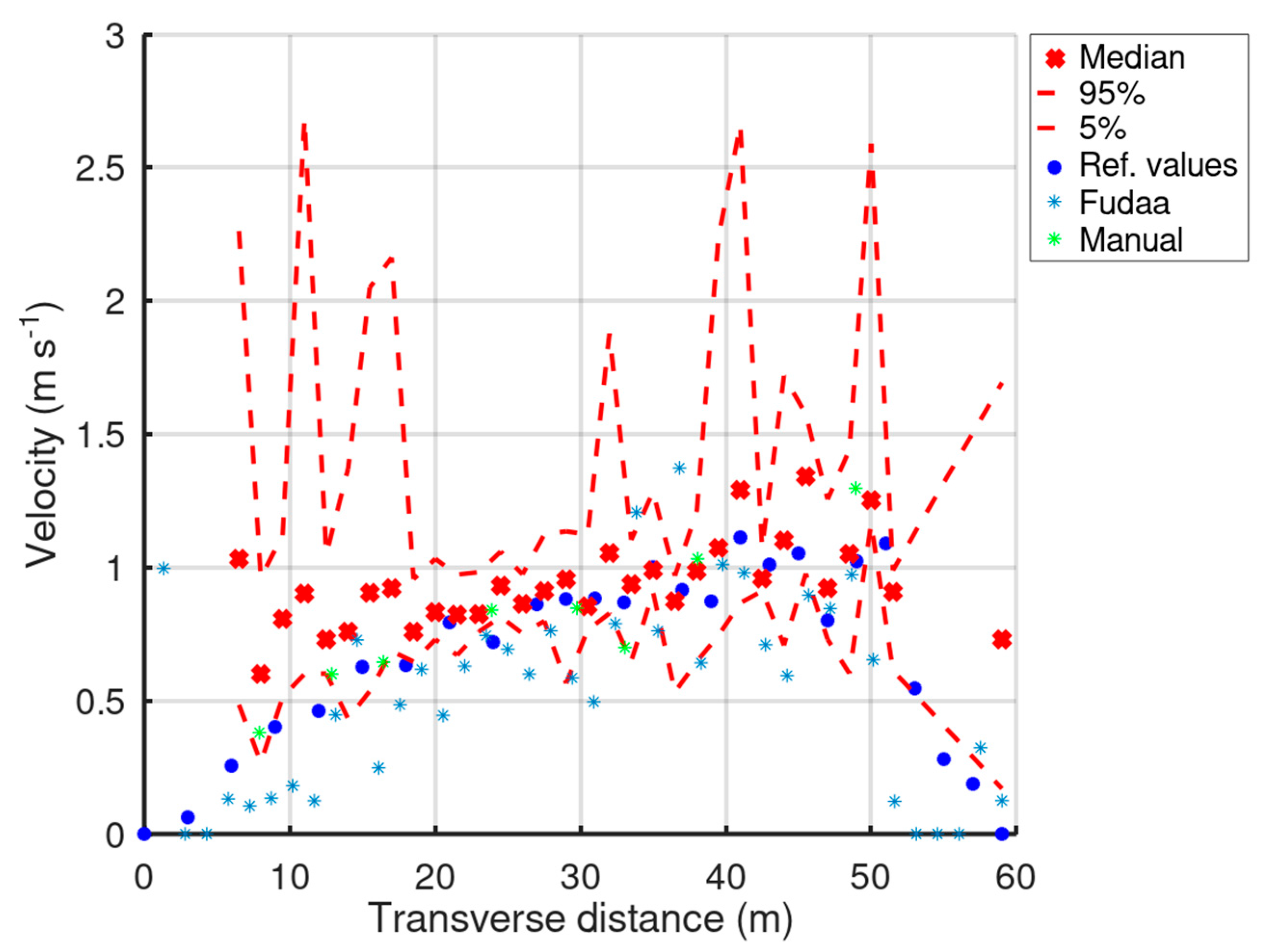
3.4. Loussios River at Atsicholos Bridge
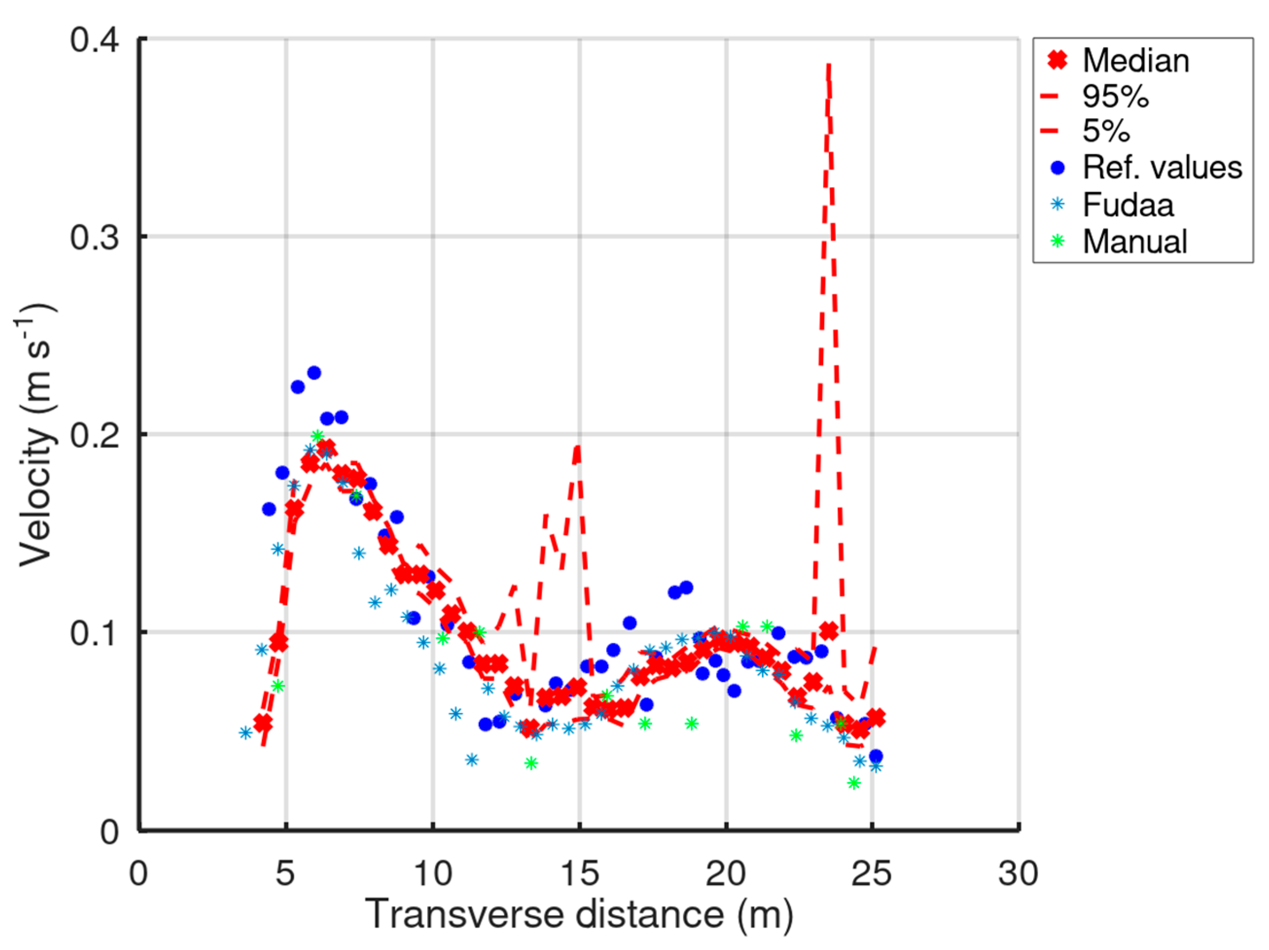
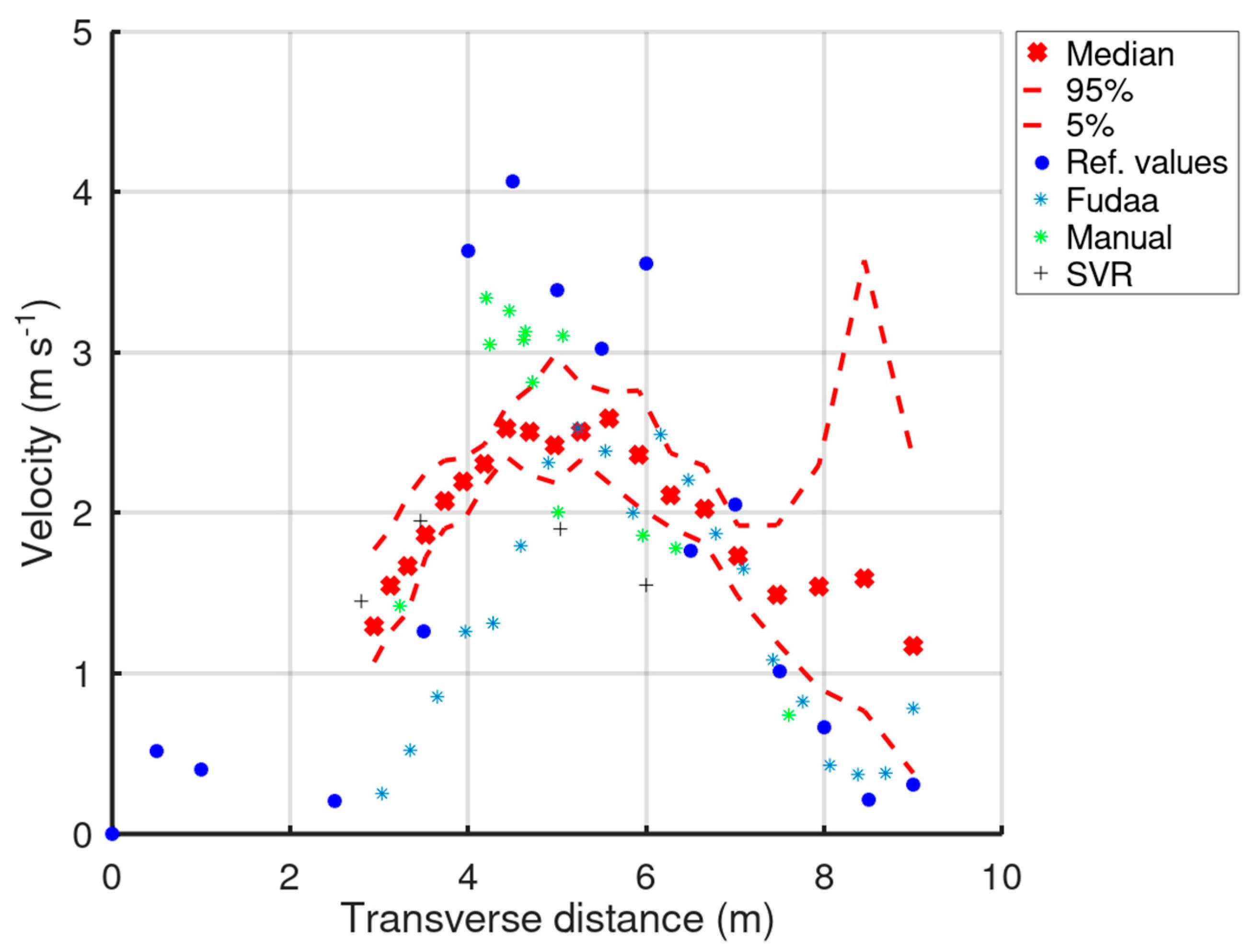
3.5. Loussios River Upstream
4. Discussion
5. Conclusions
Author Contributions
Funding
Institutional Review Board Statement
Informed Consent Statement
Data Availability Statement
Conflicts of Interest
Appendix A

| I | II | III | IV | V | |
|---|---|---|---|---|---|
| Area size (px) | 24 | 40 | 20 | 10 | 16 |
| S1 (px) | 8 | 12 | 6 | 4 | 6 |
| S2 (px) | 8 | 12 | 6 | 4 | 6 |
| S3 (px) | 8 | 12 | 20 | 4 | 6 |
| S4 (px) | 19 | 12 | 6 | 8 | 12 |
| Velocity threshold min (m s−1) | 0.02 | 0.0 | 0.0 | 0.20 | 0.1 |
| Velocity threshold max (m s−1) | 0.5 | 4.0 | 3.0 | 10.0 | 10.0 |
| Vx threshold min (m s−1) | 0.01 | −1.0 | −3.0 | 0.10 | 0.1 |
| Vx threshold max (m s−1) | 1.0 | 1.0 | −0.2 | 10.0 | 10.0 |
| Vy threshold min (m s−1) | −0.1 | −0.1 | −1.0 | −1.5 | −2.0 |
| Vy threshold max (m s−1) | 0.1 | 4.0 | 1.0 | 1.5 | 2.0 |
| Correlation min | 0.6 | 0.4 | 0.4 | 0.40 | 0.30 |
| Correlation max | 0.98 | 0.98 | 0.98 | 0.98 | 0.98 |
| I | II | III | IV | V | |
|---|---|---|---|---|---|
| IA size (px × px) | 12 × 12–48 × 48 | 30 × 30–120 × 120 | 30 × 30–120 × 120 | 11 × 11–44 × 44 | 10 × 13–40 × 52 |
| SA size (px × px) | 25 × 25–98 × 98 | 51 × 51–206 × 206 | 55 × 55–220 × 220 | 15 × 18–60 × 72 | 32 × 47–130 × 188 |
| Velocity threshold max (m s−1) | 0.5 | 4.0 | 3.0 | 3.0 | 10.0 |
| Vx threshold min (m s−1) | 0.01 | −1.0 | −3.0 | −1.5 | 0.1 |
| Vx threshold max (m s−1) | 1.0 | 1.0 | −0.0 | 3.0 | 10.0 |
| Vy threshold min (m s−1) | −0.1 | −4.0 * | −1.0 | −1.5 | −2.0 |
| Vy threshold max (m s−1) | 0.1 | 0.1 | 1.0 | 1.5 | 2.0 |
| Correlation min | 0.5–1.0 | 0.5–1.0 | 0.5–1.0 | 0.5–1.0 | 0.5–1.0 |
| Contrast | 0.3–1.0 | 0.3–1.0 | 0.3–1.0 | 0.3–1.0 | 0.3–1.0 |
Appendix B
| X Coordinate (m) | Y Coordinate (m) | Frame Row (px) | Frame Column (px) | Error * (m) |
|---|---|---|---|---|
| −3.29 | 14.33 | 391 | 271 | 0.68 |
| −1.90 | 15.67 | 380 | 393 | 0.17 |
| −0.26 | 15.70 | 374 | 513 | 0.11 |
| −3.03 | 5.06 | 724 | 68 | 0.10 |
| −1.53 | 4.75 | 757 | 368 | 0.22 |
| −0.43 | 4.88 | 808 | 617 | 0.09 |
| −2.32 | 8.70 | 521 | 345 | 0.46 |
| X Coordinate (m) | Y Coordinate (m) | Frame Row (px) | Frame Column (px) | Error (m) |
|---|---|---|---|---|
| −3.66 | 10.07 | 249 | 230 | 0.02 |
| −2.94 | 11.81 | 223 | 353 | 0.24 |
| −1.49 | 12.30 | 219 | 514 | 0.06 |
| 0.24 | 12.90 | 221 | 697 | 0.07 |
| −2.26 | 3.36 | 662 | 66 | 0.02 |
| −1.42 | 4.12 | 588 | 360 | 0.11 |
| −0.36 | 4.17 | 631 | 636 | 0.02 |
| −0.25 | 2.86 | 866 | 678 | 0.05 |
References
- Adrian, R.J. Scattering particle characteristics and their effect on pulsed laser measurements of fluid flow: Speckle velocimetry vs. particle image velocimetry. Appl. Opt. 1984, 23, 1690. [Google Scholar] [CrossRef] [PubMed]
- Dal Sasso, S.F.; Pizarro, A.; Manfreda, S. Recent Advancements and Perspectives in UAS-Based Image Velocimetry. Drones 2021, 5, 81. [Google Scholar] [CrossRef]
- Tauro, F.; Porfiri, M.; Grimaldi, S. Surface flow measurements from drones. J. Hydrol. 2016, 540, 240–245. [Google Scholar] [CrossRef] [Green Version]
- Tauro, F.; Selker, J.; van de Giesen, N.; Abrate, T.; Uijlenhoet, R.; Porfiri, M.; Manfreda, S.; Caylor, K.; Moramarco, T.; Benveniste, J.; et al. Measurements and Observations in the XXI century (MOXXI): Innovation and multi-disciplinarity to sense the hydrological cycle. Hydrol. Sci. J. 2018, 63, 169–196. [Google Scholar] [CrossRef] [Green Version]
- Fujita, I.; Muste, M.; Kruger, A. Large-scale particle image velocimetry for flow analysis in hydraulic engineering applications. J. Hydraul. Res. 1998, 36, 397–414. [Google Scholar] [CrossRef]
- Tauro, F.; Piscopia, R.; Grimaldi, S. Streamflow Observations from Cameras: Large-Scale Particle Image Velocimetry or Particle Tracking Velocimetry? Water Resour. Res. 2017, 53, 10374–10394. [Google Scholar] [CrossRef] [Green Version]
- Fujita, I.; Watanabe, H.; Tsubaki, R. Development of a non-intrusive and efficient flow monitoring technique: The space-time image velocimetry (STIV). Int. J. River Basin Manag. 2007, 5, 105–114. [Google Scholar] [CrossRef] [Green Version]
- Tauro, F.; Tosi, F.; Mattoccia, S.; Toth, E.; Piscopia, R.; Grimaldi, S. Optical Tracking Velocimetry (OTV): Leveraging Optical Flow and Trajectory-Based Filtering for Surface Streamflow Observations. Remote Sens. 2018, 10, 2010. [Google Scholar] [CrossRef] [Green Version]
- Perks, M.T.; Russell, A.J.; Large, A.R.G. Technical Note: Advances in flash flood monitoring using unmanned aerial vehicles (UAVs). Hydrol. Earth Syst. Sci. 2016, 20, 4005–4015. [Google Scholar] [CrossRef] [Green Version]
- World Meteorological Organization. Manual on Stream Gauging Vol. I Fieldwork; World Meteorological Organization: Geneva, Switzerland, 2010. [Google Scholar]
- Dal Sasso, S.F.; Pizarro, A.; Manfreda, S. Metrics for the Quantification of Seeding Characteristics to Enhance Image Velocimetry Performance in Rivers. Remote Sens. 2020, 12, 1789. [Google Scholar] [CrossRef]
- Pizarro, A.; Dal Sasso, S.F.; Perks, M.T.; Manfreda, S. Identifying the optimal spatial distribution of tracers for optical sensing of stream surface flow. Hydrol. Earth Syst. Sci. 2020, 24, 5173–5185. [Google Scholar] [CrossRef]
- Le Coz, J.; Patalano, A.; Collins, D.; Guillén, N.F.; García, C.M.; Smart, G.M.; Bind, J.; Chiaverini, A.; Le Boursicaud, R.; Dramais, G.; et al. Crowdsourced data for flood hydrology: Feedback from recent citizen science projects in Argentina, France and New Zealand. J. Hydrol. 2016, 541, 766–777. [Google Scholar] [CrossRef] [Green Version]
- Le Boursicaud, R.; Pénard, L.; Hauet, A.; Thollet, F.; Coz, J. Gauging extreme floods on YouTube: Application of LSPIV to home movies for the post-event determination of stream discharges. Hydrol. Process. 2016, 30, 90–105. [Google Scholar] [CrossRef] [Green Version]
- Le Coz, J.; Jodeau, M.; Hauet, A.; Marchand, B.; Le Boursicaud, R. Image-based velocity and discharge measurements in field and laboratory river engineering studies using the free FUDAA-LSPIV software. In Proceedings of the River Flow, Lausanne, Switzerland, 3–5 September 2014. [Google Scholar]
- Free-LSPIV: A Simple Image Velocimetry Tool. Available online: https://www.hydroshare.org/resource/e713f959ad564adf8acacf1687250ea0/ (accessed on 17 February 2022).
- Jodeau, M.; Hauet, A.; Le Coz, J.; Faure, J.B.; Bodart, G. Fudaa-LSPIV Version 1.7.3, User Manual; Document Version 04/01/2020; EDF and IRAE: France, Paris, 2020. [Google Scholar]
- Lewis, J.P. Fast Template matching. Vis. Interface 1995, 95, 120–123. [Google Scholar]
- Rozos, E.; Dimitriadis, P.; Mazi, K.; Lykoudis, S.; Koussis, A. On the Uncertainty of the Image Velocimetry Method Parameters. Hydrology 2020, 7, 65. [Google Scholar] [CrossRef]
- Gonzales, R.C.; Woods, R.E. Digital Image Processing, 2nd ed.; Prentice Hall: Upper Saddle River, NJ, USA, 2001. [Google Scholar]
- Rozos, E.; Mazi, K.; Koussis, A.D. Probabilistic Evaluation and Filtering of Image Velocimetry Measurements. Water 2021, 13, 2206. [Google Scholar] [CrossRef]
- MathWorks Help Center. Infer Spatial Transformation from Control Point Pairs. Available online: https://www.mathworks.com/help/images/ref/cp2tform.html (accessed on 15 February 2022).
- Tamari, S.; Garcia, F.; Arciniega-Ambrocio, J.I.; Porter, A. Laboratory and Field Testing of a Handheld Radar to Measure the Water Velocity at the Surface of Channels. Available online: https://www.researchgate.net/publication/260676906_Laboratory_and_field_testing_of_a_handheld_radar_to_measure_the_water_velocity_at_the_surface_of_open_channels (accessed on 15 January 2022).
- Pearce, S.; Ljubicic, R.; Peña Haro, S.; Perks, M.; Tauro, F.; Pizarro, A.; Dal Sasso, S.; Strelnikova, D.; Grimaldi, S.; Maddock, I. An Evaluation of Image Velocimetry Techniques under Low Flow Conditions and High Seeding Densities Using Unmanned Aerial Systems. Remote Sens. 2020, 12, 232. [Google Scholar] [CrossRef] [Green Version]
- Perks, M.T. KLT-IV v1.0: Image velocimetry software for use with fixed and mobile platforms. Geosci. Model Dev. 2020, 13, 6111–6130. [Google Scholar] [CrossRef]
- Perks, M.T.; Dal Sasso, S.F.; Hauet, A.; Jamieson, E.; Le Coz, J.; Pearce, S.; Peña Haro, S.; Pizarro, A.; Strelnikova, D.; Tauro, F. Towards harmonisation of image velocimetry techniques for river surface velocity observations. Earth Syst. Sci. Data 2020, 12, 1545–1559. [Google Scholar] [CrossRef]
- Hauet, A.; Morlot, T.; Daubagnan, L. Velocity profile and depth-averaged to surface velocity in natural streams: A review over a large sample of rivers. In Proceedings of the River flow, E3s Web of Conferences, Villeurbanne, France, 5–7 September 2018; EDP Sciences: Les Ulis, France, 2018; Volume 40, p. 06015. [Google Scholar]
- Detert, M.; Johnson, E.D.; Weitbrecht, V. Proof-of-concept for low-cost and noncontact synoptic airborne river flow measurements. Int. J. Remote Sens. 2017, 38, 2780–2807. [Google Scholar] [CrossRef]
- Mazi, Κ.; Koussis, A.D.; Lykoudis, S.; Vitantzakis, G.; Dimitriadis, P.; Kappos, N.; Psiloglou, B.; Katsanos, D.; Koletsis, I.; Rozos, E.; et al. HYDRO-NET: Hydro-telemetric Network for surface waters—Innovations and Prospects. In Proceedings of the EGU General Assembly 2021, Vienna, Austria, 19–30 April 2021. [Google Scholar] [CrossRef]
- Koussis, A.D.; Dimitriadis, P.; Lykoudis, S.; Kappos, N.; Katsanos, D.; Koletsis, I.; Psiloglou, B.; Rozos, E.; Mazi, K. Discharge estimation from surface-velocity observations by a maximum-entropy based method. Hydrol. Sci. J. 2022, 67, 451–461. [Google Scholar] [CrossRef]
- Blachard, S.F. Office of Surface Water Technical Memorandum 2005.05: Guidance on the Use of RD Instruments StreamPro Acoustic Doppler Profiler; Technical Report; U.S. Geological Survey: Reston, VA, USA, 2005.
- Plant, W.J.; Keller, W.C.; Hayes, K. Measurement of river surface currents with coherent microwave systems. IEEE Trans. Geosci. Remote Sens. 2005, 43, 1242–1257. [Google Scholar] [CrossRef]
- Scarano, F. Theory of non-isotropic spatial resolution in PIV. Exp. Fluids 2003, 35, 268–277. [Google Scholar] [CrossRef]
- Lei, Y.C.; Tien, W.H.; Duncan, J.; Paul, M.; Ponchaut, N.; Mouton, C.; Dabiri, D.; Rösgen, T.; Hove, J. A vision-based hybrid particle tracking velocimetry (PTV) technique using a modified cascade correlation peak-finding method. Exp. Fluids 2012, 53, 1251–1268. [Google Scholar] [CrossRef]


| Case Study | Feature Density | Feature Type | Flow Velocity | Evaluation |
|---|---|---|---|---|
| 1 | High | Artificial and fine | Low | Briefly: relatively good accuracy, medium uncertainty *. The accuracy is relatively good but is compromised by the orthorectification uncertainty which, though low in absolute terms, is significant in relative terms because of the very low flow velocity. The latter combined with the fine (instead of coarse) artificial seeding seem to be the reasons for the spikes of the upper bound of the confidence interval. |
| 2 | High | Artificial and coarse | Midrange | Briefly: very good accuracy, low uncertainty. This is the case study with the best accuracy. The flow velocity is medium and uniform, and the seeding is dense and very distinguishable. The results of the two image velocimetry algorithms practically coincide. Some of the manual estimations lay outside the confidence interval. This is not alarming; it is due to the increased variance of the instantaneous measurements, as the ADCP observations manifest, and the narrowness of the confidence interval. |
| 3 | Medium (varies) | Ripples | Midrange | Briefly: relatively good accuracy, uncertainty varies. In this case study, the accuracy is good at the middle of the cross-section, where there is good agreement between the ADV observations, the two image velocimetry methods, and the manually estimated velocities. The accuracy is low close to the banks because of the lack of detectable features on the surface. This results in the widening of the confidence interval at these locations. |
| 4 | Low | Floating debris | Midrange to high | Briefly: relatively good accuracy, medium uncertainty. In this case study, the accuracy of the image velocimetry methods is relatively good along the entire cross-section. The observed values, the estimated velocities via the image velocimetry methods, and the manual estimations all fall well within the confidence interval. |
| 5 | High | Foam, jet oscillation, roller | High | Briefly: poor accuracy, low uncertainty (deceptive a priori estimation). This case study is interesting as far as the interpretation of the image velocimetry results in case studies with similar conditions is concerned. The confidence interval is narrow and hardly includes any reference value. The image velocimetry methods underestimate the high velocities by 40%. Yet, it may be that the image velocimetry methods correctly estimate the velocity of the surface features, but the velocity of the type of features that are abundant (water foam, roller, or jet oscillation of the hydraulic jump) is not representative of the surface flow velocity. This assumption is also supported by the readings of the hand-held SVR, which are similar with the image velocimetry estimations. A possible explanation could be either the Stokes-drift effect [23] or the effect of the roughness due to the turbulence [32]. On the other hand, the error of the manual estimation, which was based exclusively on within-the-flow features (floating debris and leaves rarely occurring in the footage), was only 20%. |
Publisher’s Note: MDPI stays neutral with regard to jurisdictional claims in published maps and institutional affiliations. |
© 2022 by the authors. Licensee MDPI, Basel, Switzerland. This article is an open access article distributed under the terms and conditions of the Creative Commons Attribution (CC BY) license (https://creativecommons.org/licenses/by/4.0/).
Share and Cite
Rozos, E.; Mazi, K.; Lykoudis, S. On the Accuracy of Particle Image Velocimetry with Citizen Videos—Five Typical Case Studies. Hydrology 2022, 9, 72. https://doi.org/10.3390/hydrology9050072
Rozos E, Mazi K, Lykoudis S. On the Accuracy of Particle Image Velocimetry with Citizen Videos—Five Typical Case Studies. Hydrology. 2022; 9(5):72. https://doi.org/10.3390/hydrology9050072
Chicago/Turabian StyleRozos, Evangelos, Katerina Mazi, and Spyridon Lykoudis. 2022. "On the Accuracy of Particle Image Velocimetry with Citizen Videos—Five Typical Case Studies" Hydrology 9, no. 5: 72. https://doi.org/10.3390/hydrology9050072
APA StyleRozos, E., Mazi, K., & Lykoudis, S. (2022). On the Accuracy of Particle Image Velocimetry with Citizen Videos—Five Typical Case Studies. Hydrology, 9(5), 72. https://doi.org/10.3390/hydrology9050072