Abstract
The DRAINMOD model is a superior tool used to predict the changes in farmland water balance under different agricultural drainage layouts, fields, weather conditions, and management practices. In the present study, we assessed the sensitivity of the DRAINMOD predictions in farmland water balance to the time step (hourly or daily) in daily evapotranspiration (ET₀) computations for 12-hectares of farmland located at the lower reaches of the Yangtze River basin. The model was calibrated and validated and then was applied twice under two sets of daily ET₀ values, computed using the standardized ASCE Penman–Monteith model (one using the hourly time step (HTS) and the other using the daily time step (DTS)). Regarding daily computed ET₀ values, results show that abrupt diurnal changes in the weather always result in significant differences between daily ET₀ values when computed based on DTS and HTS. DRAINMOD simulations show that such differences between daily computed ET₀ values affected the model’s predictions of the “water fate” in the study area; e.g., adopting HTS rather than DTS resulted in a 4.8% increase, and a 3.1% and 1% decrease in the models’ cumulative predictions of runoff, drainage, and infiltration, respectively. Therefore, for a particular study area, it is critical to pay attention when deciding the best time step in ET₀ computations to ensure accurate DRAINMOD simulations, thereby ensuring better utilization of agricultural water alongside high agricultural productivity.
1. Introduction
Excess water on farmlands has always been a major threat as it causes severe crop yield losses and threatens the quality of adjacent water bodies (due to excess water runoff from such lands) [1,2,3]. Therefore, implementing artificial drainage projects in poorly drained farmlands is necessary to ensure better conditions for the agricultural process and the surrounding environment [4,5]. The best drainage layouts and practices require certain tools that could predict how current and future farmland water balances change under such layouts and practices, to achieve the desired agricultural and environmental conditions on the farmlands [6].
The DRAINMOD model is reported to be one of the best tools that enables decision-makers to predict changes in farmland water balance under different drainage layouts and practice scenarios. The model was developed by Professor Skaggs [7] at the Department of Biological and Agricultural Engineering, North Carolina (NC) State University, Raleigh, NC, and is based on water balances in the soil profile, on the field surface, and, in some cases, in the drainage system [8]. Considering the importance of the model, it is necessary to assess its sensitivity to the inputs, thereby ensuring accurate outputs and better utilization of agricultural water and environmental resources alongside high crop yields.
Potential evapotranspiration (ET₀) is one of the main inputs used by DRAINMOD when predicting water distribution patterns in a particular study area. Since the process of land potential evapotranspiration is invisible and, in most cases, complicated and expensive (in regard to being measured), many approaches have been developed to provide estimations for ET₀ values. Based on the availability of weather data (e.g., whether observed on an hourly or daily basis), these approaches compute daily ET₀ values at different time steps (e.g., daily time step (DTS) and hourly time step (HTS)). The problem is that, for a particular day, many studies, including by Jia et al. [9], Perera et al. [10], and Bakhtiari et al. [11], have reported that the daily ET₀ value computed, based on the DTS, may differ from the one computed based on the HTS. Djaman et al. [12] compared daily ET₀ values calculated on DTS and HTS for four study areas in Senegal and Guinea; the study shows that the adoption of DTS overestimated (by about 1.3 to 8%) daily ET₀ values for the whole study period relative to the ones computed based on HTS. The study also reported that, during the wintertime (November to March), the HTS-based computed daily ET₀ values tended to be higher than the DTS-based ones. The same trend was reported for the Brazilian territory; Althoff et al. [13] reported that for cold regions, the HTS-based computed daily ET₀ estimates predominantly have higher values compared to the ones computed based on DTS. In northeastern Austria, Nolz et al. [14] reported a root mean square error (RMSE) of 0.27 mm between daily ET₀ estimates, computed based on HTS and DTS. Moreover, in the State of New Mexico, the USA, Djaman et al. [15] reported RMSEs (0.21 to 0.98 mm) between the daily ET₀ values, computed based on HTS and DTS. The study also reported that the adoption of HTS resulted in higher (4.1 to 16.6%) annual ET₀ values, compared to DTS-based ET₀ estimates.
Considering the above-mentioned studies that reported such differences between daily ET₀ estimates, when the time step changes from daily to hourly, it is necessary to assess the sensitivity of DRAINMOD predictions in farmland water balance to the time step in ET₀ computations. Therefore, in the present study, we:
- Assessed the differences between daily ET₀ computations when the time step changed from daily to hourly, for 12-hectares of farmland located at the lower reaches of the Yangtze River Basin, China, from May 2018 to August 2019.
- Applied the DRAINMOD model to predict the water distribution pattern in the study area under two sets of daily ET₀ values (one computed based on DTS and the other based on HTS).
This will help to assess whether and how the DRAINMOD performance is affected by the changes in the time step in daily ET₀ computations.
2. Materials and Methods
2.1. Study Area
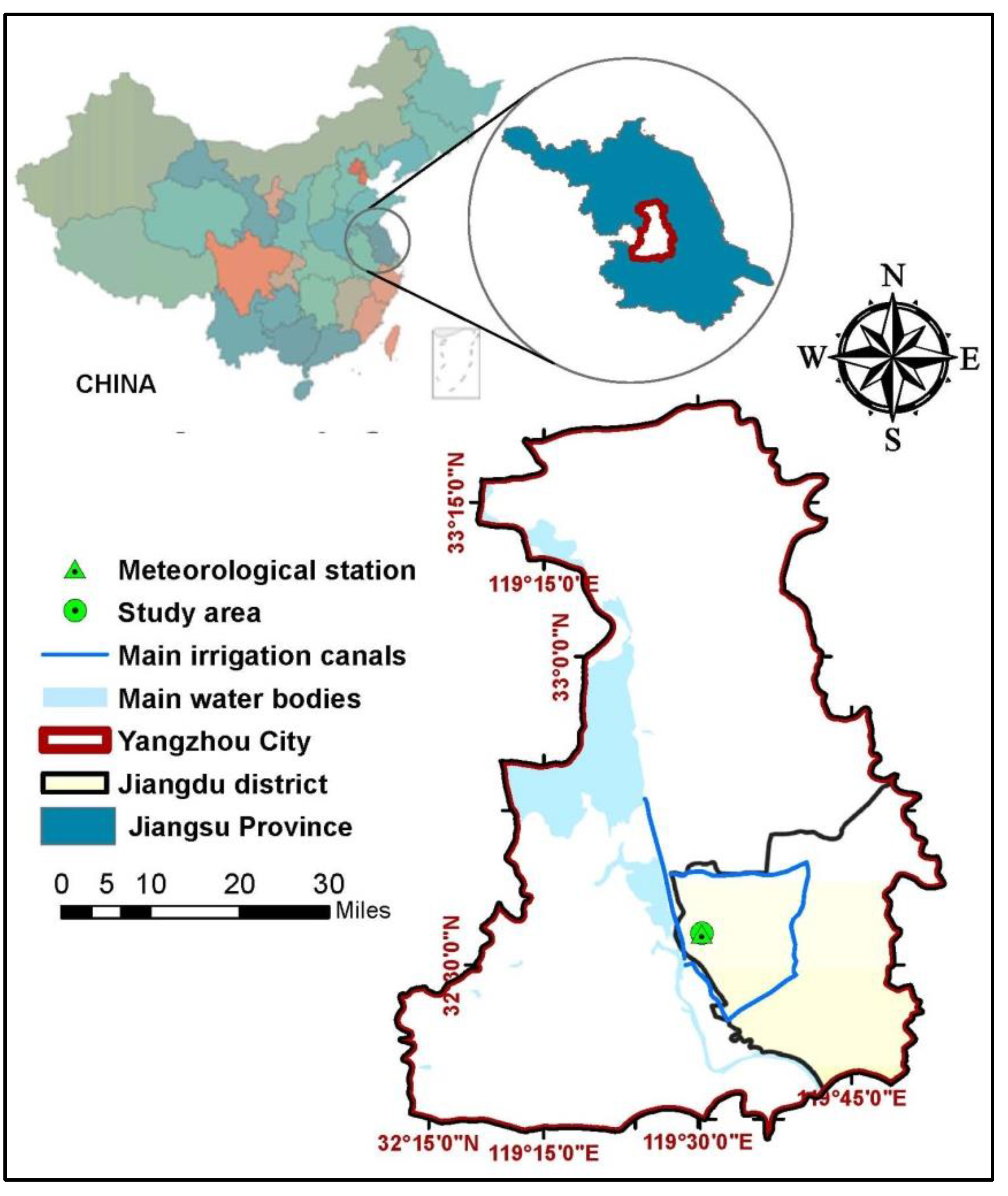
The study area is located at the lower reaches of the Yangtze River basin (YanYun irrigation District, Jiangdu District, Yangzhou, China) (Figure 1). It comprises several farmlands that have rice and wheat crop rotation. Elevations in the study area range from 5 to 8 m + mean sea level (MSL), and the annual precipitation is about 1000 mm [16].
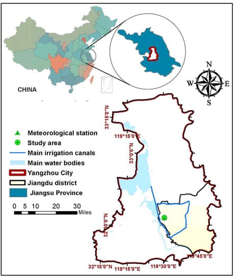
Figure 1.
The study area and location of the meteorological station.
2.2. Daily ET₀ Computations
In the present study, the American Society of Civil Engineers (ASCE) Penman–Monteith (PM) approach was used to compute daily ET₀ values based on DTS and HTS [17]. The ASCE-PM uses the same approach as the Food and Agriculture Organization (FAO)-PPM when estimating daily ET₀ values while the difference appears when adopting the HTS. When computing daily ET₀ values based on HTS, the FAO-PPM presumes a constant value for the surface resistance of vegetation per unit leaf area (rs) during all-day periods while the ASCE-PM approach presumes a smaller value of rs during the daytime and a larger value during the nighttime. Later, FAO recommended the use of rs values that were presumed in the ASCE-PM approach for daily ET₀ estimates based on HTS or other shorter periods [18].
In the present study, hourly ET₀ values were estimated following the approach developed by Snyder et al. [19]. The other necessary parameters for ET₀ estimates were computed following the approach developed by Allen et al. [20].
Collection of Weather Data Required for ET₀ Computations
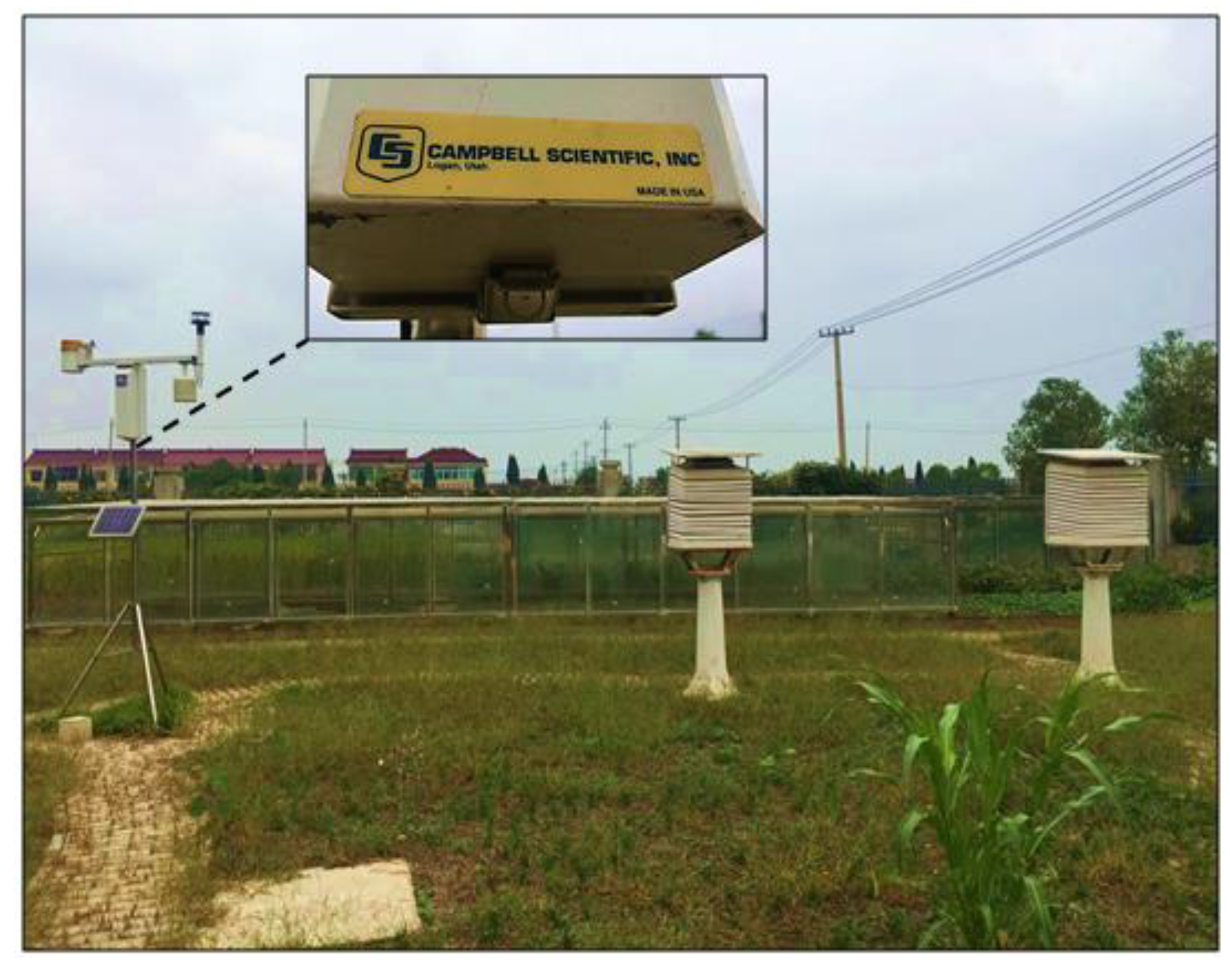
To compute daily ET₀ values, it is necessary to observe a set of weather parameters. To achieve that in the present study, a “Campbell scientific automated weather station (Figure 2)” was installed in the study area to record a wide variety of weather parameters (e.g., air temperature, precipitation, relative humidity, wind speed, solar radiation, etc.) that are necessary for ET₀ computations.

Figure 2.
Setup of the Campbell weather station in the study area with the different meteorological instruments.
2.3. DRAINMOD Simulations
2.3.1. DRAINMOD Model and Its Applications to Assess Farmland Water Balances under Different Agricultural Drainage Layouts and Practices
The model was developed mainly for field-scale applications; however, after several modifications and improvements, the model became applicable at watershed scales [21], with the ability to assess many field parameters (e.g., predictions of nitrogen and phosphorus fate in farmlands [22,23,24,25]) alongside its applicability under special environmental conditions [26]. Among the literature, there are plenty of studies (including Kladivko et al. [27], Jafari et al. [28], Nangia et al. [29], Youssef et al. [30], Wesström et al. [31], and Sands et al. [32]) in which researchers applied the model, to assess how the changes in the drainage layout (represented in drain spacing, drain depth) and drainage practices affect the “water fate” in agricultural lands. This reveals the wide use of the model as a tool that helps hydrologists assess the impacts of drainage practices in farmland water balance.
2.3.2. Potential Evapotranspiration Considerations in DRAINMOD Alongside the Data Required to Set Up and Run the Model
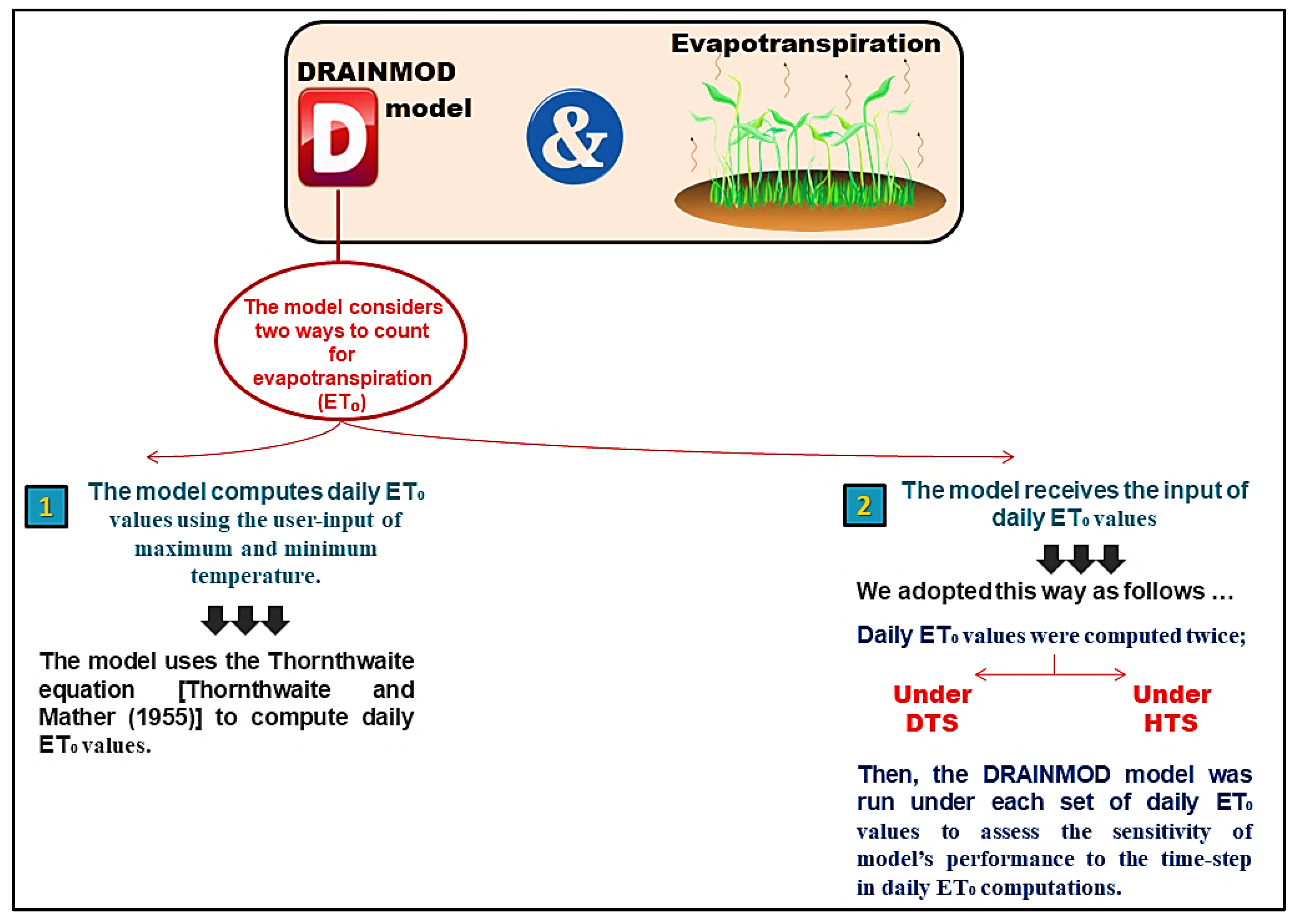
As shown in Figure 3, the DRAINMOD model was applied in the present study to predict the hydrologic regime in the study area under two sets of daily ET₀ values (one was computed using DTS and the other using HTS). This was to assess whether and how the model’s predictions of the water fate changes due to the changes in the time step in ET₀ computations.
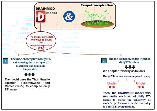
Figure 3.
The way in which DRAINMOD counts for the daily ET₀ during simulations, alongside the adopted approach, to achieve the present study’s aim.
The data required for DRAINMOD simulations can be divided into two categories:
- Data required to set up and run the DRAINMOD model.
- Data required to calibrate and validate the DRAINMOD model.
2.3.3. Data Required to Set Up and Run the DRAINMOD Model
To set up and run the DRAINMOD model, many sets of parameters related to the weather, soil, drainage system layout, management practices, etc., needed to be collected, processed (if required), and input into the model.
Weather data (in terms of daily maximum and minimum temperatures and precipitation) were collected from the installed meteorological station (Figure 2) and processed on a daily basis. The soil in the study area was loamy to silt-loam; Table 1 lists the soil properties used for DRAINMOD simulations.

Table 1.
Soil properties that were considered for DRAINMOD simulations in the present study.
Regarding the drainage layout and practices and crop pattern in the study area; the area comprises a set of open ditches spaced every 100 m alongside parallel buried pipes installed at a depth of 60 cm and spaced every 18 m. Based on observations, the average drainage flux in the study area was about 0.5 cm/d during peak drainage seasons [28]. Farmers in the study area adopt the cropping patterns of rice and wheat; rice grows from late June to early November while wheat grows from mid-November to early June. Besides the ample rainfall that characterizes the study area, irrigation is practiced during the rice-growing season to ensure the high rice water requirements. As shown in Figure 1, irrigation water is diverted from a nearby canal adjacent to the study area.
2.3.4. Data Required for DRAINMOD Calibration and Validation
In the present study, the DRAINMOD model was calibrated and validated by comparing its predictions of GWTs to the observed ones. For accurate GWT observations and, thus, better calibration and validation, the “HOBO water level data logger” was used to record groundwater depths in the study area, to have accurate observations for the calibration and validation processes of the DRAINMOD model.
The model performance was evaluated using coefficient of determination (R2) and Nash–Sutcliffe Efficiency (NSE) to measure the degree of agreement between the observed and simulated GWTs.
3. Results
3.1. Calibration and Validation of the DRAINMOD Model
DRAINMOD simulations show that the model was able to produce satisfactory predictions of GWTs in the study area (Figure 4).
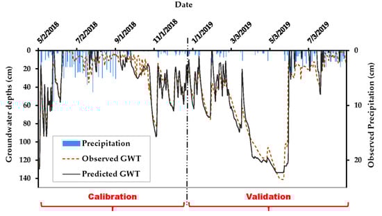
Figure 4.
Calibration and validation of the DRAINMOD model for predicting GWTs in the study area for the period May 2018 to September 2019.
Table 2 shows the agreement between the observed GWTs and those predicted by the DRAINMOD model. The good statistics indicators assure that the model can satisfactorily predict the water balance in the study area and, thus, can be applied to check the effect of any changes in input parameters (e.g., the changes in the time step in ET₀ values) on the hydrologic regime in the study area.
Table 2.
Agreement between observed GWTs and predicted ones using the DRAINMOD model.
3.2. Differences between Daily ET₀ Values as Estimated Based on DTS and HTS Alongside the Impact of These Differences on DRAINMOD Performance
3.2.1. Daily ET₀ Estimates Based on DTS and HTS
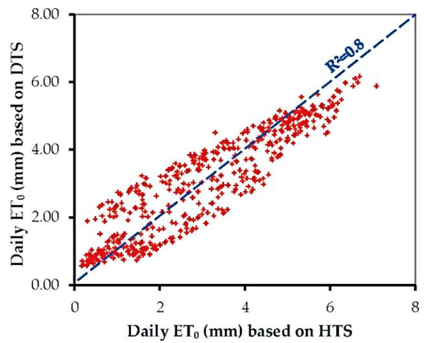
Results show that there was an overall good agreement between daily ET₀ values when computed based on DTS and HTS (Figure 5). However, during some days and months, there were large differences between DTS- and HTS-based-computed daily ET₀ values.

Figure 5.
Correlation between daily ET₀ values as computed based on DTS and HTS.
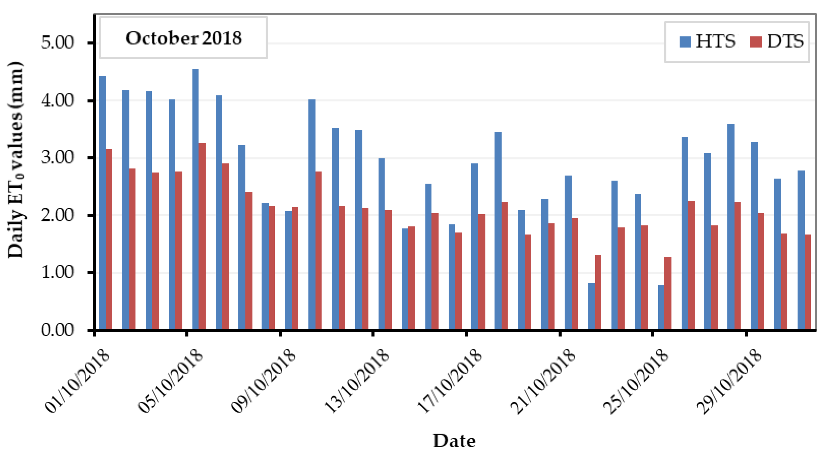
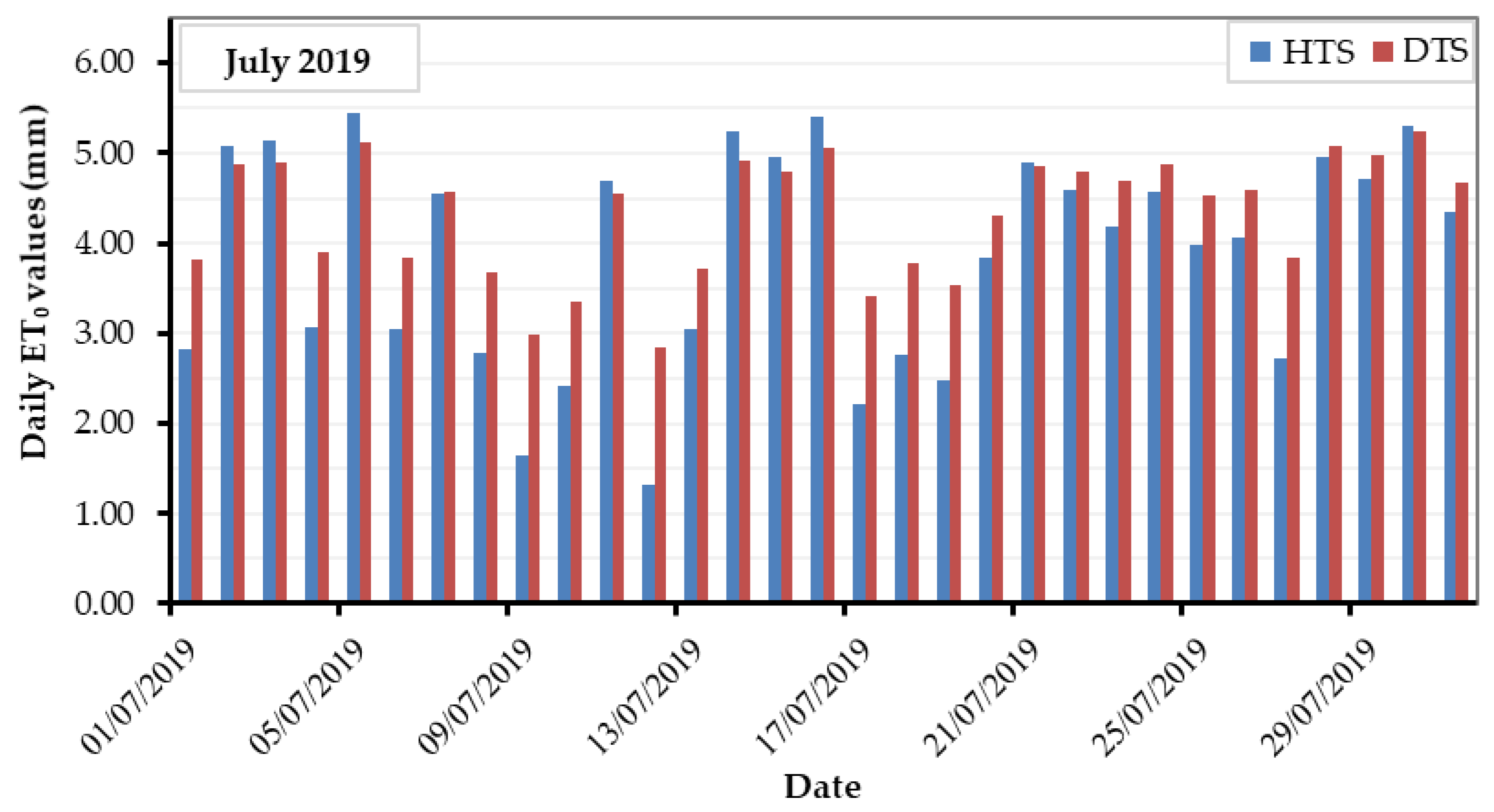
Referring to Figure 6—results revealed that during cold periods, the adoption of HTS led to higher daily ET₀ values while the opposite occurred during most hot periods. The figure shows the differences between daily ET₀ values when computed based on DTS and HTS; for October 2018 (as an example for cold periods) and July 2019 (as an example for hot periods).

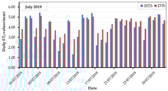
Figure 6.
Differences between daily ET₀ values as computed based on DTS and HTS; for October 2018 (as an example for cold periods) and July 2019 (as an example for hot periods).
Results also revealed that such differences between daily ET₀ values are related, much to how the weather changes during the day.
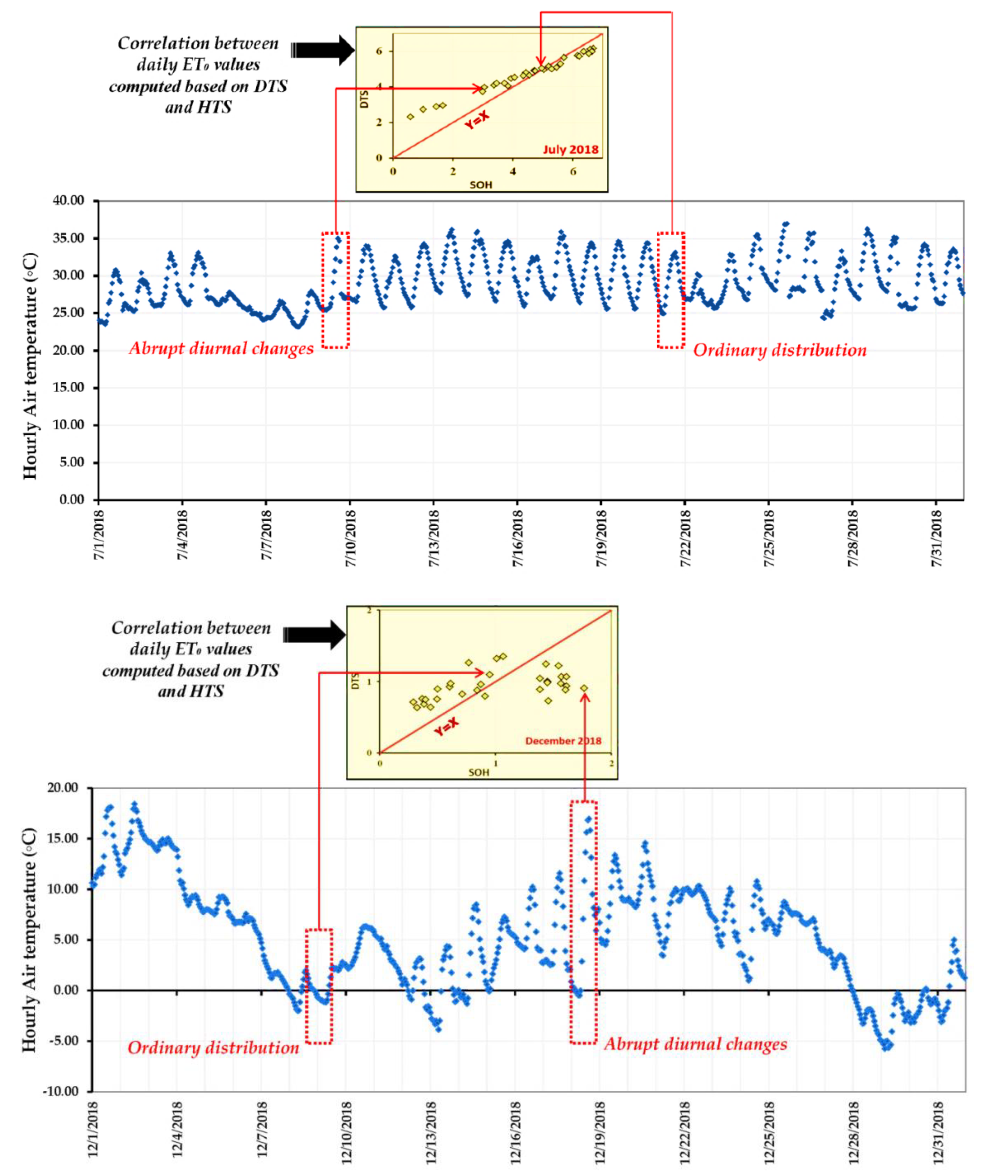
Let us consider the hourly air temperature as an example of weather parameters. Each day might show a different distribution of the hourly air temperature values; in other words, these values might change each day with a different pattern. The problem is in these days that have abrupt diurnal changes in air temperature. Based on the results, these days were predominantly found to have large differences between daily ET₀ values when the time step changed from daily to hourly. Figure 7 shows how the differences between daily ET₀ values were affected by the pattern by which the hourly air temperature values changed during the day. Two months were chosen: July 2018 (as an example of hot periods) and December 2018 (as an example of cold periods); it is clear from the figure that there are remarkable differences between the distribution patterns of hourly air temperature values in the selected months.
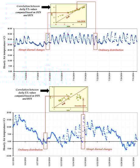
Figure 7.
Effect of the distribution pattern of the hourly air temperature values, as an example of weather parameters, on the differences between daily ET₀ values, as computed based on DTS and HTS; for July 2018 (as an example for hot periods) and December 2018 (as an example for cold periods).
The big differences between daily ET₀ values appeared in the days that have abrupt diurnal changes in the hourly air temperature values while such differences tend to be smaller on days with normal distributions of the hourly air temperature values (Figure 7).
Based on the above findings, there were slight-to-remarkable differences between computed daily ET₀ values when the time step in these computations changed from daily to hourly. Such differences have great possibility in affecting the assessment of crop water requirements [32] and, thus, the amount of water to be supplied in agricultural lands. Overestimating daily ET₀ values will result in excessive irrigation, which would create wet stresses in plants [33]. In contrast, underestimating daily ET₀ values would result in supplying agricultural lands with less water than crops need, which would create drought stresses in these crops [34]. Therefore, it is necessary to assess how such time step–change-originated differences in daily ET₀ values affect the assessment of the water fate in agricultural lands to conserve agricultural water and ensure high crop yields.
3.2.2. Sensitivity of DRAINMOD Predictions of the Water Balance in the Study Area to the Changes in the Time Step (From Daily to Hourly) in ET₀ Computations
DRAINMOD simulations show that changing the time step (from daily to hourly) in daily ET₀ computations significantly affected, in most periods, the predictions of water distribution patterns in the study area. Figure 8 shows the cumulative differences between DRAINMOD predictions of the water fate in the study area as a result from changes in the time step in ET₀ computations.
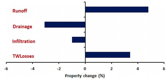
Figure 8.
Cumulative differences between DRAINMOD predictions of the water fate in the study area, resulting from the changes in the time step (from daily to hourly) in ET₀ computations.
3.2.3. A Discussion on How the Changes in DRAINMOD Predictions of the Water Fate Would Affect Agricultural Water-Use Efficiency Alongside Crop Yield
It is clear from Figure 8 that changing the time step in ET₀ computations caused the DRAINMOD model to predict a different hydrologic regime in the study area. This, without doubt, will affect the assessment of irrigation requirements in the study area, thereby agricultural production, alongside many other adverse impacts on the environment, as follows:
- Irrigation requirements and agricultural production.
Let us say that, for example, changing the time step in ET₀ computations caused the DRAINMOD model to predict higher runoff than in reality. This absolutely will make the model predict lower infiltration rates, compared to reality. As a result, the model will underestimate the soil water availability, which is the major determinate of crop water requirements.
Thus, under such a case, and based on the model simulations, the studied area would be supplied by a water amount that exceeds what is needed by crops. This may cause excess water to accumulate in the land or the root zone, creating so-called “waterlogging conditions”, which lead to induced wet stresses in crops. Thus, it is indispensable to know the most proper time step in daily ET₀ computations to ensure accurate predictions of the hydrologic regime in a particular study area, thereby ensuring better utilization of agricultural water alongside high crop yields.
- The adverse impacts on the surrounding environment.
In contrast with the above-mentioned case; let us say that, changing the time step in ET₀ computations caused the DRAINMOD model to predict low runoff compared to reality in a particular watershed. If we apply the model to manage this watershed, then the model will not be able to predict real water fluxes from farmlands to the adjacent water bodies, rather the model will predict lower runoff rates from these farmlands, compared to reality. If we rely on such model outputs, there will be a certain water amount (which is the difference between the real and predicted runoff) discharges into the adjacent water bodies and we cannot consider it or know its exact amount. This will weaken the assessment and management of the non-point source pollution [35] that is a major threat to the quality of many water bodies that surround farmlands.
4. Conclusions
The present study reported that changing the time step (from daily to hourly) in daily ET₀ computations led to small-to-remarkable differences between daily ET₀ values for a study area located at the lower reaches of the Yangtze River Basin. Such differences were affected by the patterns in which the weather changed during the day. The abrupt diurnal changes in weather parameters, compared to the rest of the day, were revealed to cause significant differences between daily ET₀ values (when computed based on daily and hourly time steps).
The DRAINMOD model was calibrated and validated in the study area and then applied to predict the water distribution pattern under the two sets of daily ET₀ computed values (one based on DTS and the other based on HTS). Results show that there was a 4.8% increase, and 3.1% and 1% decrease in DRAINMOD cumulative predictions of the runoff, drainage, and infiltration, respectively, when the time step changed from daily to hourly in ET₀ computations. This impacted the management of the irrigation process and, thereby, the crop yield.
Findings from the present study should alert hydrologists about the sensitivity of the DRAINMOD model to the time steps in daily potential evapotranspiration computations, making it better to assess the most appropriate time step to be used for a particular study area before applying a hydrological model. This would help ensure accurate water fate predictions and, thus, better utilization of agricultural water alongside high crop yields.
Author Contributions
Conceptualization, A.A.; methodology, A.A., M.E.-R. and M.A.; software, A.A., M.E.-R., M.A. and N.A.-A.; supervision, A.A.; validation, A.A; writing—original draft, A.A. and M.E.-R.; writing—review and editing, A.A., M.E.-R., M.A. and N.A.-A. All authors have read and agreed to the published version of the manuscript.
Funding
Not applicable.
Data Availability Statement
Not applicable.
Acknowledgments
The authors would like to express their sincere appreciation to the journal’s editors and anonymous reviewers for their valuable comments and suggestions. We also thank all of the lab members at the College of Water Resources and Hydropower Engineering, Yangzhou University.
Conflicts of Interest
The authors declare no conflict of interest.
References
- Ashraf, M.A. Waterlogging Stress in Plants: A Review. Afr. J. Agric. Res. 2012, 7, 1976–1981. [Google Scholar]
- Munns, R.; Goyal, S.S.; Passioura, J. The Impact of Salinity Stress. PlantStress. 2008. Available online: http://www.plantstress.com (accessed on 25 December 2021).
- Pericherla, S.; Karnena, M.K.; Vara, S. A Review on Impacts of Agricultural Runoff on Freshwater Resources. Int. J. Emerg. Technol. 2020, 11, 829–833. [Google Scholar]
- Valipour, M. Drainage, Waterlogging, and Salinity. Arch. Agron. Soil Sci. 2014, 60, 1625–1640. [Google Scholar] [CrossRef]
- Ghane, E. Agricultural Drainage; Extension Bullefin E3370. 2018. Available online: https://www.canr.msu.edu/agriculture/uploads/files/agriculturaldrainage-2-2-18-web.pdf (accessed on 28 December 2021).
- Wayne Skaggs, R. Drainage Simulation Models. Agric. Drain. 1999, 38, 469–500. [Google Scholar]
- Skaggs, R.W. Drainmod, a Water Management Model for Shallow Water Table Soils; Water Resources Research Institute of the UNC System: Raleigh, NC, USA, 1978. [Google Scholar]
- Skaggs, R.W.; Youssef, M.A.; Chescheir, G.M. Drainmod: Model Use, Calibration, and Validation. Trans. ASABE 2012, 55, 1509–1522. [Google Scholar] [CrossRef]
- Jia, X.; Steele, D.D.; Hopkins, D. Hourly Reference Evapotranspiration Estimates for Alfalfa in North Dakota. In Proceedings of the the World Environmental and Water Resources Congress 2008, Honolulu, HI, USA, 12–16 May 2008. [Google Scholar]
- Perera, K.C.; Western, A.W.; Nawarathna, B.; George, B. Comparison of Hourly and Daily Ref-erence Crop Evapotranspiration Equations across Seasons and Climate Zones in Australia. Agric. Water Manag. 2015, 148, 84–96. [Google Scholar] [CrossRef]
- Bakhtiari, B.; Khalili, A.; Liaghat, A.A.M.; Khanjani, M. Comparison of Daily with Sum-of-Hourly Reference Evapotranspiration in Kerman Reference Weather Station. J. Water Soil (Agric. Sci. Technol.) 2009, 23, 45–56. [Google Scholar]
- Djaman, K.; Irmak, S.; Sall, M.; Sow, A.; Kabenge, I. Comparison of Sum-of-Hourly and Daily Time Step Standardized Asce Penman-Monteith Reference Evapotranspiration. Theor. Appl. Climatol. 2018, 134, 533–543. [Google Scholar] [CrossRef]
- Althoff, D.; Filgueiras, R.; Dias, S.H.B.; Rodrigues, L.N. Impact of Sum-of-Hourly and Daily Timesteps in the Computations of Reference Evapotranspiration across the Brazilian Territory. Agric. Water Manag. 2019, 226, 105785. [Google Scholar] [CrossRef]
- Nolz, R.; Rodný, M. Evaluation and Validation of the Asce Standardized Reference Evapotranspiration Equations for a Subhumid Site in Northeastern Austria. J. Hydrol. Hydromech. 2019, 67, 289–296. [Google Scholar] [CrossRef] [Green Version]
- Djaman, K.; Koudahe, K.; Lombard, K.; O’Neill, M. Sum of Hourly Vs. Daily Penman-Monteith Grass-Reference Evap-otranspiration under Semiarid and Arid Climate. Irrig. Drain Syst. Eng. 2018, 7. [Google Scholar]
- Jia, Z.; Chen, C.; Luo, W.; Zou, J.; Wu, W.; Xu, M.; Tang, Y. Hydraulic Conditions Affect Pollutant Removal Efficiency in Distributed Ditches and Ponds in Agricultural Landscapes. Sci. Total Environ. 2019, 649, 712–721. [Google Scholar] [CrossRef] [PubMed]
- Allen, R.G.; Walter, I.A.; Elliott, R.; Howell, R.; Itenfisu, D.; Jensen, M. Rl Snyder, the Asce Standardized Reference Evapo-Transpiration Equation; Environmental and Water Resources Institute of the American Society of Civil: Reston, FL, USA, 2005. [Google Scholar]
- Allen, R.G.; Pruitt, W.O.; Wright, J.L.; Howell, T.A.; Ventura, F.; Snyder, R.; Itenfisu, D.; Steduto, P.; Berengena, J.; Yrisarry, J.B.; et al. A Recommendation on Standardized Surface Re-sistance for Hourly Calculation of Reference Eto by the Fao56 Penman-Monteith Method. Agric. Water Manag. 2006, 81, 1–22. [Google Scholar] [CrossRef]
- Snyder, R.; Eching, S. Pmhr Penman-Monteith Hourly Etref for Short and Tall Canopies; University of California: Davis, CA, USA, 2006. [Google Scholar]
- Allen, R.G.; Pereira, L.S.; Raes, D.; Smith, M. Crop Evapotranspiration-Guidelines for Computing Crop Water Requirements-Fao Irrigation and Drainage Paper 56; FAO: Rome, Italy, 1998; Volume 300, p. D05109. [Google Scholar]
- Fernandez, G.P.; Chescheir, G.M.; Skaggs, R.W.; Amatya, D.M. Drainmod-Gis: A Lumped Parameter Watershed Scale Drainage and Water Quality Model. Agric. Water Manag. 2006, 81, 77–97. [Google Scholar] [CrossRef]
- Brevé, M.A.; Skaggs, R.W.; Parsons, J.E.; Gilliam, J.W. Drainmod-N, a Nitrogen Model for Artificially Drained Soil. Trans. ASAE 1997, 40, 1067–1075. [Google Scholar] [CrossRef]
- Youssef, M.A.; Skaggs, R.W.; Chescheir, G.M.; Gilliam, J.W. The Nitrogen Simulation Model, Drainmod-N Ii. Trans. ASAE 2005, 48, 611–626. [Google Scholar] [CrossRef]
- Askar, M.H. Drainmod-P: A Model for Simulating Phosphorus Dynamics and Transport in Artificially Drained Agricultural Lands; North Carolina State University: Raleigh, NC, USA, 2019. [Google Scholar]
- Askar, M.H.; Youssef, M.A.; Vadas, P.A.; Hesterberg, D.L.; Amoozegar, A.; Chescheir, G.M.; Skaggs, R.W. Drainmod-P: A Model for Simulating Phosphorus Dynamics and Transport in Drained Agricultural Lands. I. Model Development. Trans. ASABE 2021, 64, 1835–1848. [Google Scholar] [CrossRef]
- Luo, W.; Skaggs, R.W.; Chescheir, G.M. Drainmod Modifications for Cold Conditions. Trans. ASAE 2000, 43, 1569. [Google Scholar] [CrossRef]
- Kladivko, E.J.; Frankenberger, J.R.; Jaynes, D.B.; Meek, D.W.; Jenkinson, B.J.; Fausey, N.R. Nitrate Leaching to Subsurface Drains as Affected by Drain Spacing and Changes in Crop Production System. J. Environ. Qual. 2004, 33, 1803–1813. [Google Scholar] [CrossRef]
- Jafari-Talukolaee, M.; Shahnazari, A.; Ahmadi, M.Z.; Darzi-Naftchali, A. Drain Discharge and Salt Load in Response to Subsurface Drain Depth and Spacing in Paddy Fields. J. Irrig. Drain. Eng. 2015, 141, 04015017. [Google Scholar] [CrossRef]
- Nangia, V.; Gowda, P.H.; Mulla, D.J.; Sands, G.R. Modeling Impacts of Tile Drain Spacing and Depth on Nitrate-Nitrogen Losses. Vadose Zone J. 2010, 9, 61–72. [Google Scholar] [CrossRef] [Green Version]
- Youssef, M.A.; Abdelbaki, A.M.; Negm, L.M.; Skaggs, R.W.; Thorp, K.R.; Jaynes, D. B Drainmod-Simulated Performance of Controlled Drainage across the Us Midwest. Agric. Water Manag. 2018, 197, 54–66. [Google Scholar] [CrossRef]
- Wesström, I.; Joel, A.; Messing, I. Controlled Drainage and Subirrigation—A Water Management Option to Reduce Non-Point Source Pollution from Agricultural Land. Agric. Ecosyst. Environ. 2014, 198, 74–82. [Google Scholar] [CrossRef]
- Sands, G.R.; Song, I.; Busman, L.M.; Hansen, B.J. The Effects of Subsurface Drainage Depth and Intensity on Nitrate Loads in the Northern Cornbelt. Trans. ASABE 2008, 51, 937–946. [Google Scholar] [CrossRef]
- Klt, K. Plant Growth and Yield as Affected by Wet Soil Conditions Due to Flooding or Over-Irrigation. 2004. Available online: http://irrigationtoolbox.com/ReferenceDocuments/Extension/Nebraska/g1904.pdf (accessed on 28 December 2021).
- Farooq, M.; Wahid, A.; Kobayashi, N.S.M.A.; Fujita, D.B.S.M.A.; Basra, S.M.A. Plant Drought Stress: Effects, Mechanisms and Management. In Sustainable Agriculture; Springer: Berlin/Heidelberg, Germany, 2009; pp. 153–188. [Google Scholar]
- Ritter, W.F.; Shirmohammadi, A. Agricultural Nonpoint Source Pollution: Watershed Management and Hydrology; CRC Press: Boca Raton, FL, USA, 2000. [Google Scholar]


Publisher’s Note: MDPI stays neutral with regard to jurisdictional claims in published maps and institutional affiliations. |
© 2022 by the authors. Licensee MDPI, Basel, Switzerland. This article is an open access article distributed under the terms and conditions of the Creative Commons Attribution (CC BY) license (https://creativecommons.org/licenses/by/4.0/).