Article

Forecasting High-Flow Discharges in a Flashy Catchment Using Multiple Precipitation Estimates as Predictors in Machine Learning Models

by
Andre D. L. Zanchetta
1,*,
Paulin Coulibaly
1,2 and
Vincent Fortin
3
1
Department of Civil Engineering, McMaster University, 1280 Main Street West, Hamilton, ON L8S 4L7, Canada
2
School of Earth, Environment and Society, McMaster University, 1280 Main Street West, Hamilton, ON L8S 4L7, Canada
3
Meteorological Research Division, Environment and Climate Change Canada, 2121 Route Transcanadienne, Dorval, QC H9P 1J3, Canada
*
Author to whom correspondence should be addressed.
Hydrology 2022, 9(12), 216; https://doi.org/10.3390/hydrology9120216
Submission received: 26 October 2022 / Revised: 23 November 2022 / Accepted: 29 November 2022 / Published: 30 November 2022
(This article belongs to the Section Hydrological and Hydrodynamic Processes and Modelling)

Abstract

:
The use of machine learning (ML) for predicting high river flow events is gaining prominence and among its non-trivial design decisions is the definition of the quantitative precipitation estimate (QPE) product included in the input dataset. This study proposes and evaluates the use of multiple concurrent QPEs to improve the performance of a ML model towards the forecasting of the discharge in a flashy urban catchment. Multiple extreme learning machine (ELM) models were trained with distinct combinations of QPEs from radar, reanalysis, and gauge datasets. Their performance was then assessed in terms of goodness of fit and contingency analysis for the prediction of high flows. It was found that multi-QPEs models overperformed the best of its single-QPE counterparts, with gains in Kling-Gupta efficiency (KGE) values up to 4.76% and increase of precision in detecting high flows up to 7.27% for the lead times in which forecasts were considered “useful”. The novelty of these results suggests that the implementation of ML models could achieve better performance if the predictive features related to rainfall data were more diverse in terms of data sources when compared with the currently predominant use of a single QPE product.

1. Introduction

1.1. Background

Floods are among the most hazardous events for human life and infrastructure. According to estimations from the United Nations, their occurrence increased by more than 50% in the current decade following an upward trend apparently driven by climate change [1]. Different regions of the world face regular threats of hazardous flooding driven by intense precipitation, e.g., the seasonal Monsoon Asia [2,3,4], the mountainous regions of Italy [5] and of China [6], and urbanized regions of the United States [7] and of Brazil [8]. To support the decisions of emergency response teams, governmental agencies implement flood early warning systems (FEWS), which are characterized as integrated components designed for hazard monitoring, forecasting, disaster risk assessment and communication [9,10].
The river discharge forecasting component of FEWSs historically rely on conventional hydrological models (CHMs) to predict river discharges through simulations of physical or conceptual representations of the hydrological cycle [11,12]. As data-driven alternatives for CHMs, the potential of using supervised machine learning (ML) models for tasks related to rainfall-runoff modelling has been studied for more than 25 years [13,14]. Driven by a continuously increasing of data and computational power availability, an expanding number of ML methods and algorithms has been explored with success, with performances comparable or superior to their CHM counterparts [15]. Examples of ML structures already applied for such a purpose include multi-layer perceptrons (MLP) [16,17], long-short term memory neural networks (LSTM) [18,19], random and decision tree forests [20,21], support vector machines (SVM) [22,23] and extreme learning machines (ELM) [24,25]. This scenario motivates the exploration of techniques and approaches to improve their performance for an implementation in operational forecasting chains [26].
Unsurprisingly, rainfall is usually considered one of the dominant factors determining the occurrence of floods [27]. Replicating the design approach adopted for CHMs, in which each input data represents univocally a material or energetic flux relevant for the local hydrological processes, ML models have been trained and tested with quantitative precipitation estimates (QPE) derived from a single source, be it from rain gauges [19,22], ground-based weather radar [28] or satellite data [29,30]. However, each of such products has specific advantages and limitations: rain gauges are considered the most accurate estimator of rainfall water depth while being restricted to provide measurements for point locations; ground-based weather radars are able to provide relevant information about the spatial distribution and motion of rainfall by recording microwaves reflected from the upper atmosphere, which results in elevated uncertainties concerning the amount of precipitated water that reaches the ground; and numerical weather models (NWM) include concepts of physics to fill gaps and bridge different sources of observational data, potentially adding epistemic uncertainties to the estimated rainfall value [31,32].
These differences usually raise questions on which of these estimations is the best to be used to represent precipitation as input in discharge forecasting systems. They also motivate the search for techniques for combining different QPEs in a way to efficiently maintain their positive characteristics and mitigate their errors. The combination of multiple QPEs is usually performed separately from the rainfall-runoff simulation model, in an additional component that produces a single and supposedly improved QPE. The post-processed QPE is then used as the input for the rainfall-runoff model [33,34]. The use of a post processor external to the hydrological model, however, has the drawbacks of (1) increasing the complexity of an operational systems, as two components need to be set up and maintained, and of (2) assuming that one of the rainfall products (usually from rain gauges) is available and has a quality high enough to be considered a reference for the other QPEs, which may become a constraint for data scarce regions. If a rainfall-runoff model could encapsulate both the QPE combination and the discharge estimation components through data-driven methods (thus without prior assumptions on the data quality of individual products), both the drawbacks would be overcome.
Different from CHMs, conventional ML models are designed to abstractly identify patterns in the training dataset, can be constructed to have an arbitrary number of inputs, and are not constraint by physical laws or conceptualizations of the hydrological behavior of a catchment. This flexibility allows the construction of models that estimates future discharge having multiple concurrent precipitation estimates as part of its input. Such a configuration fulfils the suggested encapsulation, however, to the best of the author’s knowledge, no previous work has investigated the potential effectiveness of including more than one source of QPE products in the predictors set for improving discharge forecasting in ML models.

1.2. Research Questions and Objectives

The purpose of this work is to answer the question: can the use of concurrent QPE products improve the performance of rainfall-runoff ML models? And, more specifically: can it improve the prediction of high flows?
The novelty of the paper is to present and evaluate the hypothesis that ML tools can be efficient on identifying how underlying patterns in concurrent QPE products is reflected in the discharge of a small catchment. This hypothesis raises the expectations that the more QPE products used as predictive features, the higher can be the performance of the model. However, the inclusion of an additional predictor highly correlated with other input data may not result in performance gains and thus leading to an unjustified increase in the model complexity. Even worse: it can result in the overfitting of the data-driven model and consequently in the deterioration of the model performance. Such a duality is usually referred to as “the curse of dimensionality” [35] and demands case-specific analysis on whether a feature should be included or not, which justifies the need for the study presented in this paper.
Answering the abovementioned research questions can serve as an important factor for designers of river forecasting systems based on artificial intelligence, particularly on their decision to consider (or not) using predictor sets composed by more than one rainfall product instead of relying on the use of single QPEs as usually observed in the literature. While the experiment is performed in a densely monitored catchment, the insights presented can also benefit the development of models of poorly gauged or ungauged basins given the current availability of multiple precipitation products with global coverage that could be used as a replacement for the gauged data in this study.
For evaluating our hypothesis, a computational experiment was conducted to compare the performance of different ELMs models, each taking distinct sets of precipitation estimates as input. The conventional single-QPE design is included in the comparison to represent the business-as-usual approach, and the Don River Basin, located in Toronto, Canada, is taken as a study case.

2. Materials

2.1. Study Area

The densely occupied Don River basin (Toronto, ON, Canada) houses approximately 1.4 million residents in total area of nearly 350 km2 upstream the river gauge HY019 (Figure 1), where the average baseflow is estimated to be in the order of 5 m3/s. The longest flow path has 38 km length and an average slope of 6.6 × 10⁻³, which reflects the overall smoothness of the relief in the surroundings of the Great Lakes.
The response time of the catchment at the gauge HY019 is about 3 h, therefore the Don River basin can be considered “flashy” according to the criterion adopted by the United States’ National Weather Service for defining flash floods, i.e., floods “beginning within six hours of the causative event (e.g., intense rainfall, dam failure, ice jam)” [36]. Despite the shape of the basin being relatively elongated, with its two main branches (East and West Don Rivers) being almost parallel for the most of their length, the catchment presents a rapid response time due to its high level of urbanization (over 80%) and insufficient number of stormwater management control structures [37], which derives from an urbanization process that predates modern structural practices.
Located in a humid continental climate zone (Köppen climate classification Dfa), the precipitation regime is characterized by the occurrence of more intense rainfall events during the warm season (from May to October) and reduced precipitation records during the remaining of the year, with an average annual cumulative precipitation of about 660 mm [38].
The area just downstream the gauge HY019, known as “lower Don”, frequently becomes flooded due to river overbank conditions triggered by intense precipitation events during the warm season of the years. Such flooding scenarios recurrently result in disturbances in the operation of high-traffic roads and urban railways in the riverside of the lower Don, causing significant economical and material losses, besides overall life-threatening conditions for the local population.

2.2. Dataset

2.2.1. Data Description

The discharge data (Q) used was collected by the stream gauge HY019. Four meteorological stations equipped with tipping buckets and located within (or close to) the catchment (HY016, HY021, HY027, HY036 as shown in Figure 2) recorded the data used as a representative of rain gauge estimates (referred as G). The Toronto and Region Conservation Authority (TRCA) is the agency responsible for managing the Don River Basin, for maintaining all the above-mentioned gauges, and for providing the collected data to the public at 15 min temporal resolution.
QPEs from data collected by the National Oceanic and Atmospheric Administration (NOAA) NEXRAD S-Band weather radar located in Buffalo, USA, were used to represent products from ground-based radars (referred as R). The distance between the station and the most distant point of the catchment is 128 km, which is within the usable range of 180 km from this ground-based weather radar [39]. The specific product used, referred as N1P, is calculated by NOAA’s Precipitation Processing System algorithm [40] and provided at temporal and spatial resolutions of 1 h and approximately 2 km over the Don River basin, respectively.
The Canadian Precipitation Analysis (CaPA) products produced by the Environment and Climate Change Canada (ECCC) in its 10 km, hourly resolution version [41] is used as the NWM representative (referred as C). The version of CaPA products used in this work integrates observation data from North American Surface Synoptic Observations (SYNOP), Surface Weather Observations (SWOB) and METeorological Aerodrome Reports (METAR) gauge networks with numerical weather simulations based on the ECCC’s Global Environmental Multiscale model (GEM) [42]. It is worth noting that the aforementioned gauge networks do not include stations maintained by TRCA. A summary of the dataset is given in Table 1.

2.2.2. Data Pre-Processing

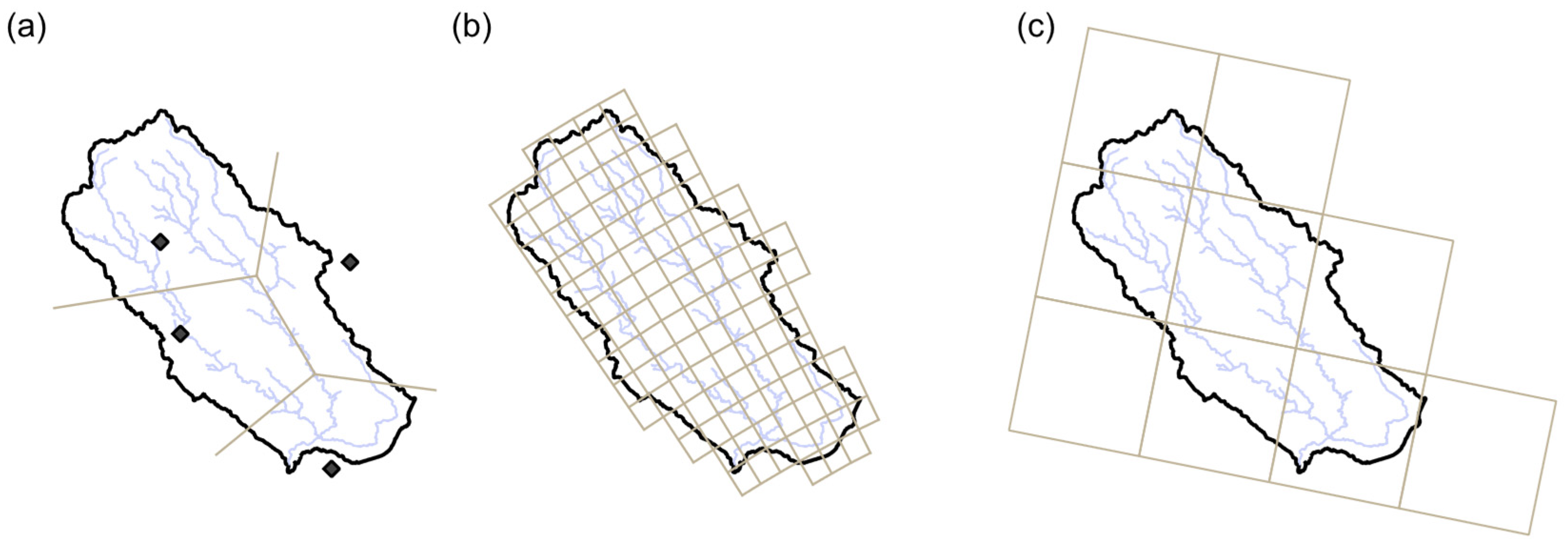
The radar and the NWM products were used “as-is”. The decision of not applying common data treatments (such as bias correction) is based on the assumption that the ELM is capable of “learning” by its own the characteristics and patterns of the raw QPE products that are relevant to the task of predicting stream discharge. All precipitation records were spatially aggregated into a single uniform value following a lumped representation of the catchment given its small area. Particularly, the rain gauge data was aggregated using the conventional Thiessen polygons method [43] and the weights of each gauge in the weighted average is given in Table 2. The spatial granularity of the different precipitation products over the Don River basin is presented in Figure 2.
All timeseries were temporarily aggregated into hourly resolution to match the resolution of the CaPA data as it is the coarsest among the products considered. A total of 63 intense rainfall-runoff events observed in the warm seasons between the years of 2011 to 2017 were identified and used to compose the train/validation/test dataset. A rainfall-runoff event is considered intense when the discharge posterior to a rainfall record exceeds 10 times the baseflow value, and each event is defined in time as the 24 h interval centered in the peak discharge.

3. Methods

3.1. Extreme Learning Machine (ELM) Models

ELM models [44] are single-layer feed-forward neural networks that are calibrated analytically instead of through the conventional stochastic gradient descent approach. In a summary, the output y for an input x produced by an already trained ELM is given by:
y ( x ) = i = 1 N h ω i   F i ( x ) = i = 1 N h ω i   f ( s ( α i , x ) ) = i = 1 N h ω i   f ( j = 1 N x α i , j x j )  
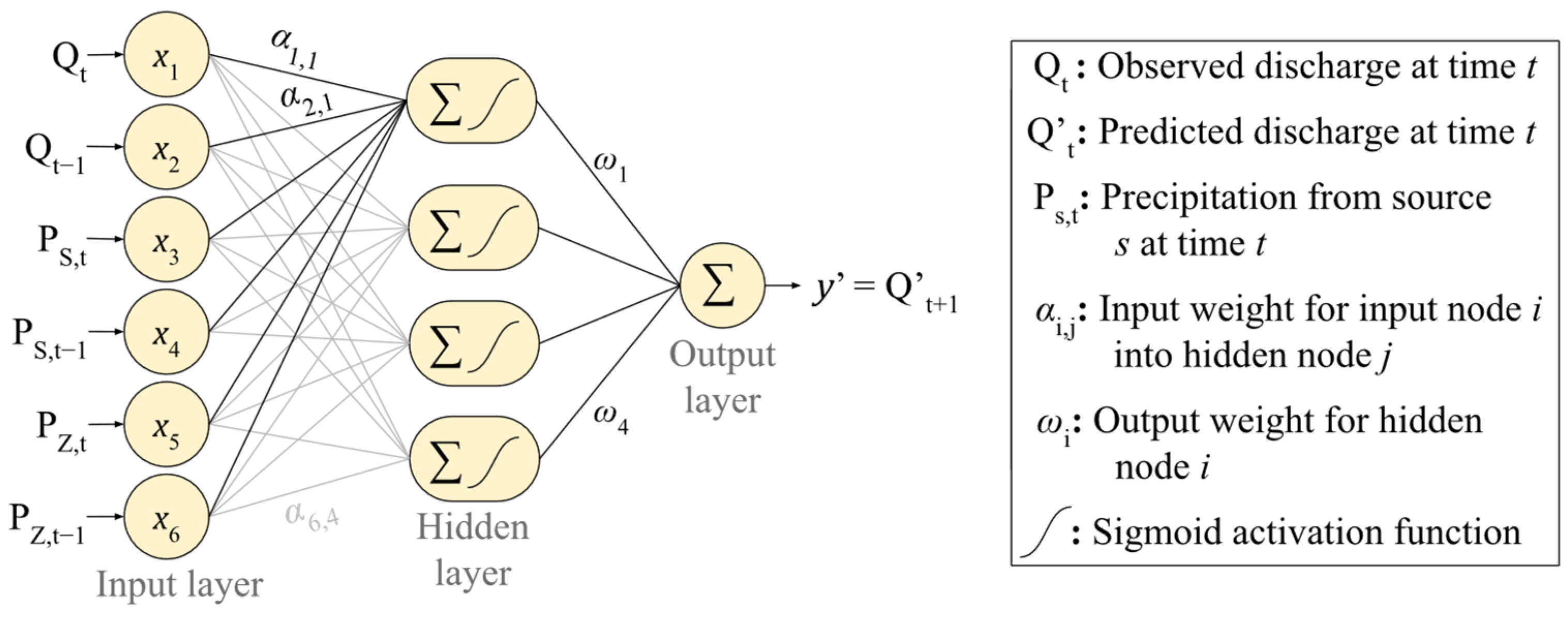
in which N h   is the number of hidden neurons; the output value and output weight of the i-th hidden node are given by F i and ω i , respectively; F i is calculated as the output of the activation function f for the weighted sum s of x ; α i is the input weights for the i-th hidden node; both x and α i have N x components; and the j-th components x and α i is represented by x j and α j , i , respectively. A visual representation of the structure is given in Figure 3.
As a data-driven model, the tuning of an ELM is performed by fitting its intrinsic mathematical formula (in the form of Equation (1)) using a set X of N t training samples ( x 1 , x 2 , …, x N t ) as arguments and a set Y of their respective target values ( y 1 ,   y 2 , ,   y N t ) . The set H ( X ) of output values of the hidden layers for all samples in X , the set W of output weights of the hidden nodes, and Y can be represented in matrices as:
H ( X ) = [ F 1 ( x 1 ) F N h ( x 1 ) F 1 ( x N t ) F N h ( x N t ) ] ,   W = [ ω 1 ω N h ]   and   Y = [ y 1 y N t ]
so that the vectorial representation of the solutions for the training sample is given by:
Y = H ( X ) × W
As previously discussed, the function F is parameterized by the input-to-hidden node weights ( α j , i of Equation (1)). In ELM, a random value is set for each α j , i and are kept constant, which makes W the only unknown to be defined during the training stage. The inverse of H ( X ) , H ( X ) + , is obtained through the Moon-Penrose generalized inversion function so that an approximation W is calculated as:
W = H ( X ) + × Y
The values of W ( ω 1 , ω 2 , …, ω N h ), which were therefore defined using the training sets X and Y , are used as the calibrated values of ω 1 , ω 2 ,…, ω N h in Equation (1). As discussed by Huang et al. [44], such an approach provides the minimum training error, calculated as least-square error, for a network characterized by its number of hidden nodes and activation functions. In this work, we used ELM with the sigmoid activation function based on previous successful application on rainfall-runoff modelling [25,45], while the number of nodes in the hidden layer is considered a hyperparameter.

3.2. Experiment Set Up

A total of 8 sets of inputs were composed by all possible combinations of the 3 QPE products considered ([G], [R], [C], [G, R], [G, C], [R, C], [G, R, C], [None]) and two records of antecedent discharge ( Q t L and Q t L 1 ). For each input set and for each lead time L ranging from 1 to 5 h, multiple ELM models were trained to map the predictors P t L , P t L 1 , Q t L , Q t L 1 to the predictand instant discharge Q t ( t being an instant time and P the univariate, multivariate or absent QPE in the input set).
As ELM models are fit analytically to the data used for training, they are known to be highly prone to overfitting and conventional generalization methods designed for in iterative trainings, like early stopping [46], are not applicable. The approach adopted for overcoming this issue is to use the mean of the outputs of an ensemble of ELM predictors and with each of the ensemble members being fit to a different subset of the training data, as presented by Liu and Wang [47]. In this work, for creating the ensemble of models and for testing them, a nested k-fold cross validation approach was adopted.
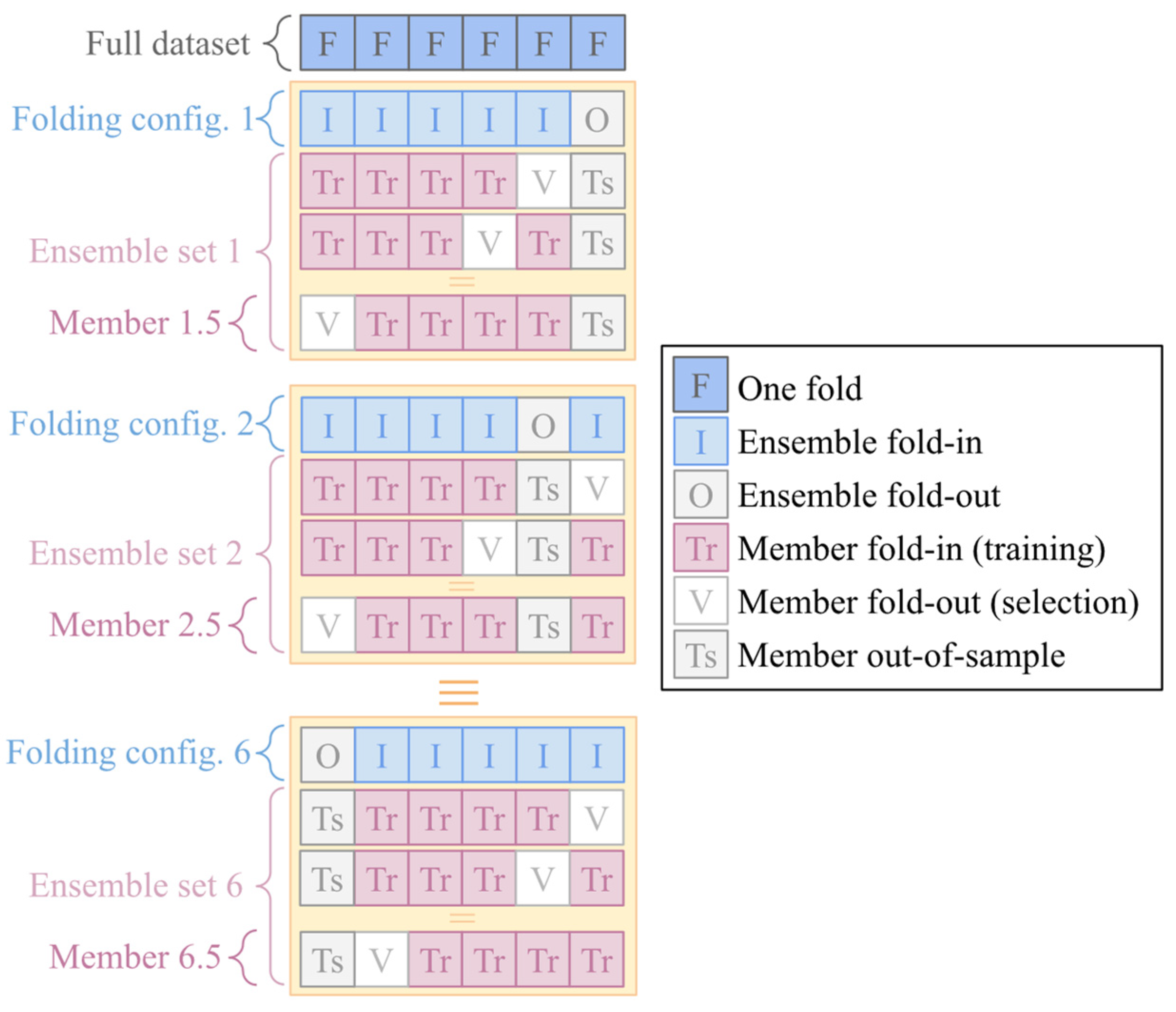
The entire dataset was randomly segmented in 6 folds (subsets) so that each possible combination of 4 folds (66.6% of the data) can be used to train one individual ML model using 1 of the other folds for testing (16.7% of the data) and the 1 remaining fold for validation (16.7% of the data). Such a data splitting schema was adopted to resemble the data distribution of 70% for training and 30% for testing/validating as commonly adopted in the literature [48,49,50]. Based on such a data division, 6 ensemble sets of ELM models were set up, each of the ensembles having a folding configuration in which 5 of the subsets are used for training its ensemble members (ensemble fold-in), and the remaining subset is reserved for testing the ensemble forecasts (ensemble fold-out, or “member out-of-the-sample”). The 5 ensemble folds-in of each folding configuration are used to fit 5 ELM models, each ELM model using 4 of the folds for producing multiple ELM model candidates (member fold-in) and the remaining fold (member fold-out) to select the trained candidate with best generalization power. A visual representation of the aforementioned data splitting is given in Figure 4.
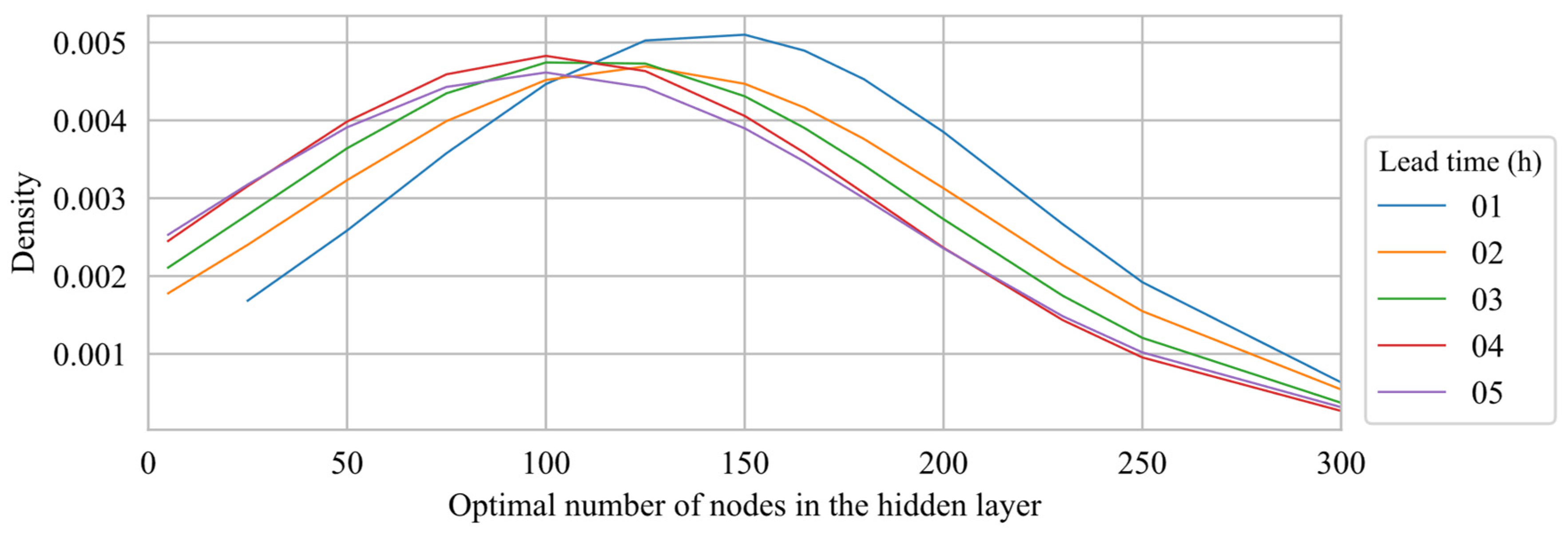
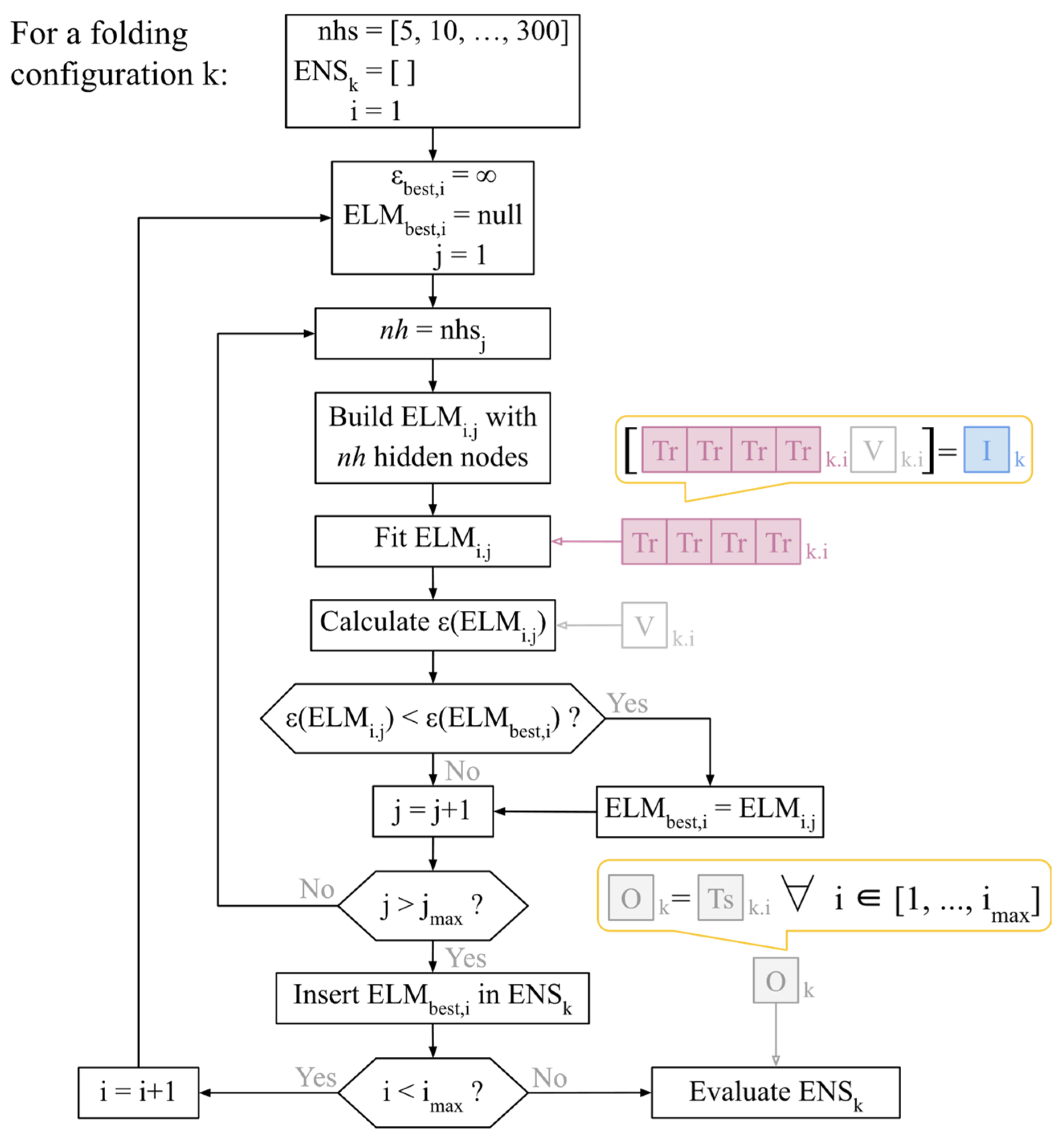
To tune the only hyperparameter of the ELM models (i.e., the number of nodes in the hidden layer), multiple ELM candidate models for each member fold-in subset were trained, each of which having a different number of hidden nodes ranging from 5 to 300. The candidate model that presented the best performance in terms of lower root mean squared error (RMSE) using the respective member fold-out is selected. The aforementioned range of explored number of nodes in the hidden layer was determined from preliminary empirical experiments based on try and error (not shown). As it can be observed in Figure 5, the mean number of hidden nodes selected as optimal are between 100 and 150 depending on the lead time to which the ML models are trained, with only a very limited portion of the models having between 250 and 300, which indicates that the range of total number of nodes explored was adequate for this problem. Each density function aggregates all individual models trained for each lead time, regardless its input set and its ensemble group.
After the fitting and the hyperparameter tunning, for each of the 6 folds of the entire dataset, an ensemble of 5 ELM models is set up using only data from the other folds. The comparison of the model ensembles is performed using the data in the fold that was not included in the training/validation/selection stage (i.e., member out-of-the-sample), as represented in Figure 6.

3.3. Models Comparison

The overall performance of the models trained with different predictors were compared in terms of goodness of fit using Pearson’s correlation coefficient ( r , Equation (4)) [51], root mean squared error (RMSE, Equation (5)) [52] and the Kling-Gupta Efficiency (KGE, Equation (6)) [53]. In a summary: r measures the linear correlation between the predicted and observed discharge values, assuming values between −1 (perfect inverse correlation) to 1 (perfect direct correlation), with the value 0 indicating total absence of linear correlation between the variables; RMSE represents the square root of the average of squared error of a prediction dataset, has values in the same units as the evaluated variable (m3/s in this work) and range from 0 to infinity (the higher, the worse); and KGE is an efficiency metric that balances the agreement between the predicted and observed values in terms linear correlation, standard deviation and mean, with unitless values bounded between 0 (worse agreement possible) and 1 (perfect agreement). Additionally, fractional bias (Equation (7)) [52] is used to estimate the magnitude of the systematic overestimation (if value is positive) or underestimation (if value is negative) of the ELM models.
The above-mentioned metrics are calculated as:
r = i = 1 N ( Q i Q i ¯ ) × ( Q 1 Q i ¯ ) i = 1 N ( Q i Q i ¯ ) 2 × i = 1 N ( Q i Q i ¯ ) 2   ,
R M S E = i = 1 N ( Q i Q i ) 2 N   ,
K G E = 1 ( r 1 ) 2 ( µ µ 1 ) 2 ( σ σ 1 ) 2 ,
F r a c t i o n a l   b i a s = 2 N i = 1 N Q i Q i Q i + Q i .
in which Q i and Q i are, respectively, the i -th observed and i -th predicted discharges; N is the total number of records in Q i and Q i ; μ and μ are the mean of the Q and Q values, respectively; and σ   and   σ are the standard deviation of Q and Q , respectively.
Contingency metrics of critical success index (CSI, Equation (8)), sensitivity (also known as “recall”, Equation (9)) and precision (Equation (10)) were used to assess the applicability of the model to predict high-flow events. In this work, a high-flow event is an individual moment in time during an intense rainfall-runoff event in which Q exceeds 50 m3/s, equivalent to 10 times the baseflow discharge. The contingency metrics used in this work take into account the total of observed high-flow events that were correctly predicted ( h i t s ), the total of observed events that were not predicted ( m i s s e s ), and the total of events that were predicted but not observed ( f a l s e   a l e r t s ) as:
C S I = h i t s h i t s + m i s s e s + f a l s e   a l e r t s   ,
s e n s i t i v i t y = h i t s h i t s + m i s s e s   ,
p r e c i s i o n = h i t s h i t s + f a l s e   a l e r t s   .

4. Results and Discussion

4.1. Overall Performance Statistics

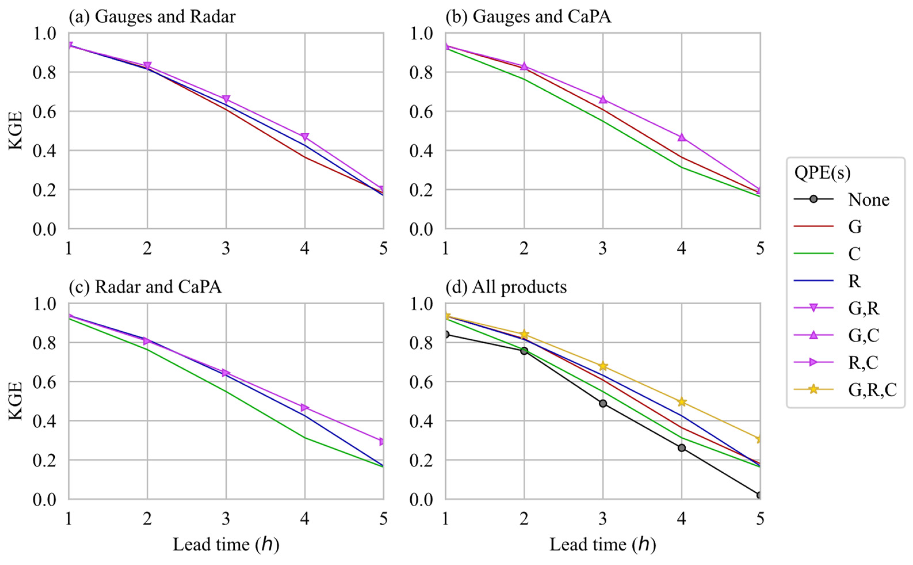
The average performance of the different ELM ensemble models in terms of KGE is presented in Figure 7. As expected, the ELM models that uses none of the QPEs presented the worst performance among all input configurations considered, with absolute KGE differences of up to 0.14 when compared with the worst-performing single-QPE models (Figure 7d). This observation illustrates the magnitude of gains in performance that the ELM models can attain by “learning”, up to a certain level, the influence that precipitation has on the discharge of the catchment for the different lead times.
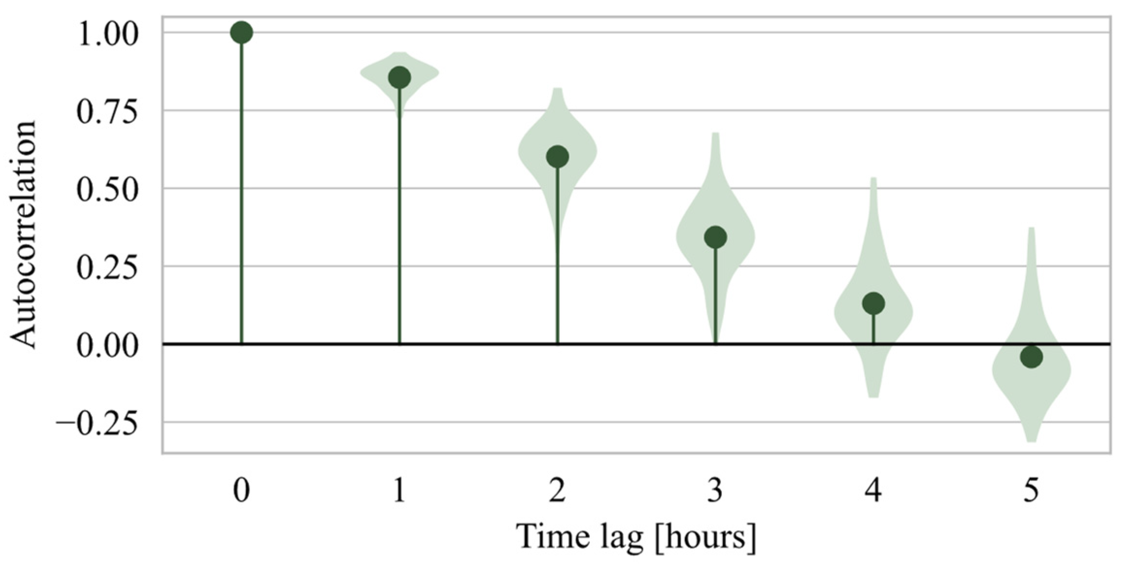
Among the single-QPE ELM models, the ones using radar data presented the best performance in terms of KGE for lead times of 3 and 4 h, and a performance comparable with the ELM that uses only gauges data for the other lead times. ELM models using CaPA data presented lower performance for lead times of 2, 3 and 4 h when compared with its radar-based counterpart. A remarkable characteristic of the KGE values of all single-QPE ELMs is their comparable performances for both the shortest (1 h) and longest (5 h) lead time. A probable explanation for such a pattern may be related to the response time of the catchment of approximately 3 h. The water that enters the catchment as precipitation in a moment t tends to have limited influence on the discharge at the outlet of the catchment in a moment t + 1 h as the majority of its volume is still in transit through the basin. Most of the runoff volume reaches the outlet between t + 2 h and t + 4 h, thus differences in precipitation patterns are more likely to be reflected in the discharge at these instants. At t + 5 h, most of the water entering at time t is expected to have already left the catchment, leading to a condition similar to t + 1. The major decrease in performance of the models with lead time L is likely driven by the Q t L and Q t L 1 predictors (present in all models) following their decaying correlation with the predicted variable Q t as L increases (Figure 8).
All ELM models that use two of the QPE products concurrently presented equal or higher KGE values than the models that use only one of the QPEs individually (Figure 7a–c). The differences in performance between the single-QPE models and the two-QPE models is almost imperceptible for the shortest lead time. For longer lead times, the gain in performance with the use of more precipitation input varied for each pair of QPE products. Gains in absolute KGE are up to 0.04 for the gauge and radar pair (Figure 7a), up to 0.11 for the gauge and CaPA pair (Figure 7b) and up to 0.12 for the radar and CaPA pair (Figure 7c).
As observed for the two-products scenarios, the models that use all QPEs presented a better performance than the best single-QPE models for all lead times, except for t + 1 h, when the differences are imperceptible (Figure 7d).
Taylor diagrams created using the Python library Skill Metrics [54] summarize the statistical parameters of standard deviation, coefficient of correlation with observations, and RMSE of the ELM models that use no QPE, the ones that use only one QPE product, and the ones that use all three QPEs (Figure 9). As observed in the KGE analysis, the models using the three QPE products performed in average better or as good as their best single-QPE counterparts for all lead times except for 1 h, in which all QPE-aware ELMs practically coincide in all the three metrics. This consistency in the results from different metrics is a good indicator that the gains in performance with additional QPEs are not concentrated in specific scenarios nor produce undesired significant drawbacks.
Table 3 summarizes the mean of the main metrics for evaluating the goodness-of-fit of the models, including the percentual gain of using the three QPEs when compared to the best performing single-QPE models. Out of the 15 scenarios (KGE, RMSE and r metrics at 5 lead times each), the multi-QPE did not present the best performance in only 1 (RMSE at 1 h lead time), had a performance comparable to the best of the single-QPE model in other 2 scenarios (KGE and r at 1 h lead time), and was the best in the remaining 12 scenarios, making it the “clear winner” in terms of overall performance.
As presented in Table 4, the set of models that consider only radar data presented the lowest bias among the single-QPE group of models. Nevertheless, when all the three QPE products are used as input, a reduction in the overall bias is observed for all lead times. It worth noting, though, that all model setups are characterized as being biased low (negative bias value), a pattern that can be due to the fact that each predicted value used is the mean of an ensemble of model outputs, which tends to lead to a “smoothening” of the predictions, especially for the peak values. As improvements were also observed in other metrics, it is possible to deduce that the use of multiple QPE products resulted in an appropriate increase of the overall values predicted (higher bias value).
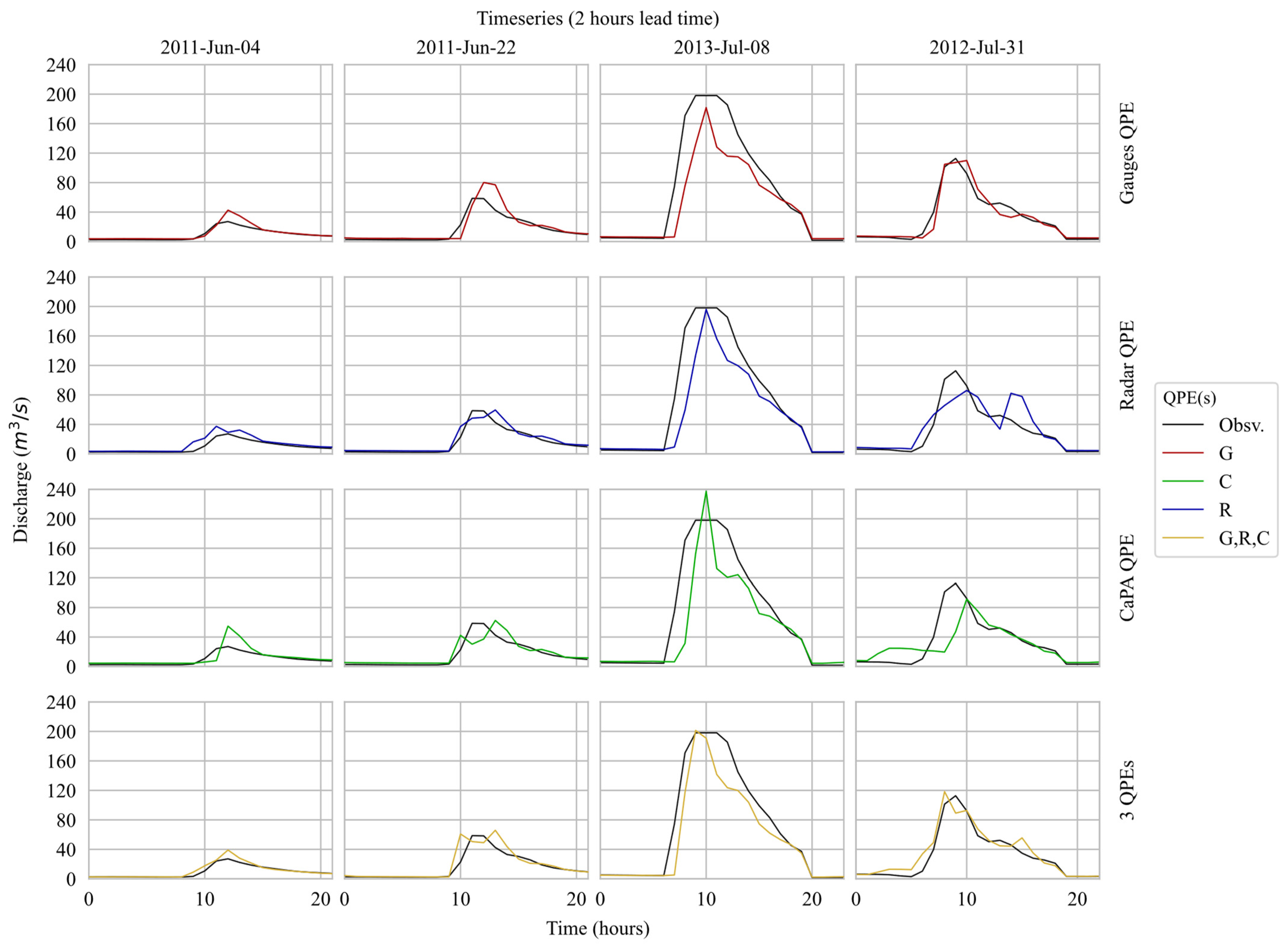
The hydrographs of four distinct high-flow events presented in Figure 10 reflect the patterns identified in the performance metrics, i.e., multi-QPEs models usually outperforming its single-QPE counterparts. One component to be highlighted is the timing: in all events except the one of 4 June 2011, the three-QPEs models was the one to earliest predict the peak, event even anticipating in one hour the maximum flow observed in one hour. Such an anticipation may eventually be considered a positive characteristic for first responders as they have more time to act.
These results answer our first research question by evidencing that ML models indeed have the potential to “learning” patterns in the rainfall data estimated by different sources concurrently and improve their performance in reproducing rainfall-runoff processes. Additionally, it is possible to note that if a ML designer is constrained to use a single QPE product, discussions may rise on which data source should be chosen depending on the metrics considered. For example: models using only radar data and models using only gauge data were each considered as “the best model” for 2 lead times in terms of RMSE and r , while for KGE, radar-based models overperformed gauge-based models with a tight difference (3 times the first overperforming the later against 2 the other way around).

4.2. Contingency Analysis

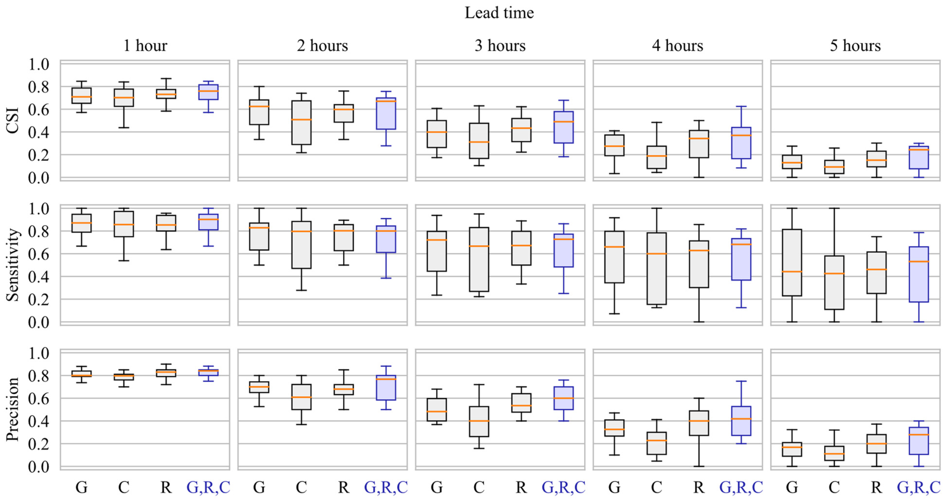
As described in Section 3.3, the threshold adopted in this study to identify high-flows events was the value representing 10 times the baseflow discharge (i.e., 50 m3/s), and the calculated contingency metrics for the identification of high-flows events is presented in Figure 11. For all lead times, the EML models that use the three QPE products as predictors presented a median CSI value that is higher than its best-performing single-QPE counterparts, which indicates an overall best performance of the first over the later on predicting the upcoming occurrence of a high-flow record. Reflecting the results obtained in the analysis of the goodness of fit, the single-QPE model that uses CaPA products consistently presented the worst results. Models using only gauge and only radar data presented competitive performances between each other, with the first performing better in lead times of 2 h while the later overperformed in the remaining lead times.
The boxplots representing the sensitivity values of the models that use multiple QPEs have little differences when compared to the boxplots of its best-performing single-QPE counterpart. The forecast precision of all models remains high for lead time 1 and 2 h at about 75% and then deteriorate significantly for subsequent lead times. If the criterion for deciding if an ensemble of models is that both precision and sensitivity should be higher than 0.5, the maximum lead time to which they could be deemed “useful” is 3 h. The resulting CSI values of the models that use multiple precipitation inputs is the highest (or equivalent to other highest model with only one precipitation product) for all lead times—indicating the superior potential benefit in using all precipitation products.
The performance of single-QPE and three-QPE models for detecting high flows is summarized in Table 5. If only the ability to anticipate the occurrence of an upcoming high-flow event is to be considered, regardless of the number of false alarms issued, modelers could be inclined to select the models that use only QPEs from gauges as their sensitivity was the highest for 2 of the lead times. On the other hand, if avoiding the emission of false alarms is the main interest for the forecasters, the single-QPE model that uses only radar data overcomes its gauge data-based counterpart for the majority of the lead times due to its best performance in terms of precision. However, usually both the sensitivity and precision of forecasting models are important, and a balanced metric such as CSI is used as tiebreaker. In this work, however, CSI values indicate, as observed with KGE, that the radar-based ELMs overperform the gauges-based ELMs with just 3 out of the 5 lead times, which could still rise questions in the selection of the single-QPE product to be used.
The three-QPEs models overperformed the other three single-QPE ones in terms of precision for all led times, scored equally to the best ELMs (the ones using gauge data only) in two of the lead times and underperformed it in the remaining three lead times. If CSI is used as a tiebreaker, the three-QPEs configuration would emerge as a “clear winner” as it presents the best metrics for 4 out of 5 lead times though. Taking the single-QPE model that uses radar data as a reference, it is possible to interpret from these results that the addition of the other precipitation products provided useful information for skillfully reduce the number of false alarms issued, thus increasing the precision of the model in a way that outweighs the reduction of the number of missed events. These results answer our second question: using concurrent QPE as input of the ML models also improved the prediction of high-flow events mainly by increasing its precision.

4.3. Brief Discussion on Replicability

The replicability of the results presented in Section 4.1 and Section 4.2 is yet to be assessed for other densely monitored catchment covered by multiple systems that provide QPEs. This is a scenario usually observed in urban areas of significative economical or societal relevance, but still unlikely for most of the basins [55].
With recent technological developments, however, different systems now provide QPEs with global or sub-global coverage. Examples of such precipitation products available in near-real time include the estimates derived from satellites, such as the Integrated Multi-satellitE Retrievals for Global precipitation measurement (IMERG) [56], the Global Satellite Mapping of Precipitation (GSMaP) [57], and the Precipitation Estimation from Remotely Sensed Information using Artificial Neural Networks—Cloud Classification System (PERSIAN-CCS) [30,58,59]. Individual satellite-based precipitation data usually presents coarse spatio-temporal resolution and, as any other QPE product, different sources of uncertainty, which results in the task of performing discharge forecasting for poorly gauged or ungauged basins challenging and subject of research. The findings of this work may also motivate developers of machine learning models for rainfall-runoff forecast to consider the possibility of using multiple QPE products from different global datasets to enhance model performance when an appropriate rain gauge monitoring network is absent.

5. Conclusions

The performance of machine learning models to predict high-flow river discharge has the potential to benefit from the concurrent use of different QPE products in the input set of features when compared to the business-as-usual configuration of a single source for QPEs. For the “flashy” and small urban catchment taken in this work as study case, the model using three QPE products presented an overall goodness of fit to the observed discharge that outperformed the best single-QPE models for most of the forecasted lead times (ranging from 1 to 5 h in the future) and metrics (KGE, coefficient of correlation, RMSE and bias) evaluated. For anticipating high river flows, the multi-QPE models tended to present a better trade-off between number of errors of false alarms and missed events when compared to each of their best-performing single-QPE counterparts. The eventual performance loss usually expected when highly correlated variables are used as predictors of data-driven models (due to overfitting or excessive increase in model complexity) were overcome by the gains in considering the complementary information provided by each individual QPE source. Thus, our study suggests that if a region is served by more than one precipitation estimate, which is becoming more feasible due to the consolidation of the different satellite-based programs, then it worth considering the use of multiple QPEs as predictors of ML-based rainfall-runoff models. Therefore, the answer to the question “which of the available QPEs should be used to reach the best overall performance?” may be just “all of them” when using ML models to predict stream discharges.
The gains in performance observed, however, are limited by the information available in the input data as only three QPE products were considered. Additionally, results were presented only using one machine learning technique and for only one gauged catchment in which summer floods are mainly driven by intense rainfall followed by nearly instant surface runoff, and in which the influence of other hydrological factors such as soil moisture and evapotranspiration can be neglected.
Considering the aforementioned limitations of this work, future studies are recommended for exploring:
  • How the use of multiple precipitation products may benefit poorly gauged or ungauged basis using QPEs based on satellite data (e.g., PERSIANN-CCS, IMERG, GSMaP);
  • How does the performance of ML-based rainfall-runoff models that use multiple concurrent QPEs as input compares with the performance of conventional hydrological models that use a post-processed QPE based on the combination of different QPE products (e.g., radar data corrected with gauged data);
  • What are the potential gains in performance that rainfall-runoff models based on other popular ML structures (e.g., MLP, LSTM, SVM, random forests) may achieve with the inclusion of concurrent QPEs in the set of predictors;
  • How the ML-based rainfall-runoff modeling of basins with characteristics different from the flashy urban catchment used in this study may benefit from the use of multiple concurrent QPEs as input. Examples of such include mountainous catchments and non-flashy basins with larger areas.

Author Contributions

Conceptualization, implementation, and writing—original draft preparation, A.D.L.Z.; writing—review and editing, supervision, project administration, funding acquisition, P.C.; data acquisition, supervision, writing—review, V.F. All authors contributed equally to the discussion over the results and contributed to the final manuscript. All authors have read and agreed to the published version of the manuscript.

Funding

This research was funded by Natural Science and Engineering Research Council of Canada (NSERC), grant NETGP-451456.

Institutional Review Board Statement

Not applicable.

Informed Consent Statement

Not applicable.

Data Availability Statement

Weather Radar data: retrieved from the National Centers for Environmental Information (NCEI) Archive Information Request System (https://www.ncei.noaa.gov/has/HAS.DsSelect, accessed on 2 February 2022). CaPA data: retrieved from CaSPAr (https://caspar-data.ca/caspar, accessed on 2 February 2022). Rain and stream gauged data were provided by TRCA and ECCC, respectively. Access to these datasets is subject to consent of their providers.

Acknowledgments

TRCA for providing the precipitation data recorded by rain gauges, ECCC for providing the revised discharge data used in this work.

Conflicts of Interest

The authors declare no conflict of interest.

Abbreviations

AcronymMeaning
CaPACanadian Precipitation Analysis
CHMConventional Hydrological Model
CSICritical Success Index
ECCCEnvironment and Climate Change Canada
ELMExtreme Learning Machine
GEMGlobal Environmental Multiscale
KGEKling-Gupta Efficiency
LSTMLong-Short Term Memory
METARMETeorological Aerodrome Reports (METAR)
MLMachine Learning
NOAANational Oceanic and Atmospheric Administration
NWMNumerical Weather Model
QPEQuantitative Precipitation Estimate
RMSERoot Mean Squared Error
TRCAToronto and Region Conservation Authority

References

  1. UN-Water United Nations World Water Development Report 2020: Water and Climate Change; UNESCO: Paris, France, 2020; ISBN 9789231003714.
  2. Sanyal, J.; Lu, X.X. Remote Sensing and GIS-Based Flood Vulnerability Assessment of Human Settlements: A Case Study of Gangetic West Bengal, India. Hydrol. Process. 2005, 19, 3699–3716. [Google Scholar] [CrossRef]
  3. Sanyal, J.; Lu, X.X. Application of Remote Sensing in Flood Management with Special Reference to Monsoon Asia: A Review. Nat. Hazards 2004, 33, 283–301. [Google Scholar] [CrossRef]
  4. Ghosh, S.; Hoque, M.M.; Islam, A.; Barman, S.D.; Mahammad, S.; Rahman, A.; Maji, N.K. Characterizing Floods and Reviewing Flood Management Strategies for Better Community Resilience in a Tropical River Basin, India. Nat. Hazards 2022. [Google Scholar] [CrossRef]
  5. Corral, C.; Berenguer, M.; Sempere-Torres, D.; Poletti, L.; Silvestro, F.; Rebora, N. Comparison of Two Early Warning Systems for Regional Flash Flood Hazard Forecasting. J. Hydrol. 2019, 572, 603–619. [Google Scholar] [CrossRef] [Green Version]
  6. Zhai, X.; Guo, L.; Liu, R.; Zhang, Y. Rainfall Threshold Determination for Flash Flood Warning in Mountainous Catchments with Consideration of Antecedent Soil Moisture and Rainfall Pattern. Nat. Hazards 2018, 94, 605–625. [Google Scholar] [CrossRef]
  7. Habibi, H.; Dasgupta, I.; Noh, S.; Kim, S.; Zink, M.; Seo, D.J.; Bartos, M.; Kerkez, B. High-Resolution Hydrologic Forecasting for Very Large Urban Areas. J. Hydroinf. 2019, 21, 441–454. [Google Scholar] [CrossRef]
  8. Fonseca Alves, L.G.; de Oliveira Galvão, C.; de Farias Santos, B.L.; Fernandes de Oliveira, E.; Andrade de Moraes, D. Modelling and Assessment of Sustainable Urban Drainage Systems in Dense Precarious Settlements Subject to Flash Floods. LHB Hydrosci. J. 2022, 108, 1–11. [Google Scholar] [CrossRef]
  9. WMO—World Meteorological Organization. Multi-Hazard Early Warning Systems: A Checklist. In Proceedings of the Outcome of the first Multi-hazard Early Warning Conference, Cancun, Mexico, 22–23 May 2017. [Google Scholar]
  10. UN—United Nations. Report of the Open-Ended Intergovernmental Expert Working Group on Indicators and Terminology Relating to Disaster Risk Reduction; report A/71/644; United Nations: New York, NY, USA, 2016. [Google Scholar]
  11. Zahmatkesh, Z.; Kumar Jha, S.; Coulibaly, P.; Stadnyk, T. An Overview of River Flood Forecasting Procedures in Canadian Watersheds. Can. Water Resour. J. 2019, 44, 213–229. [Google Scholar] [CrossRef]
  12. Zanchetta, A.D.L.; Coulibaly, P. Recent Advances in Real-Time Pluvial Flash Flood Forecasting. Water 2020, 12, 570. [Google Scholar] [CrossRef] [Green Version]
  13. Minns, A.W.; Hall, M.J. Modélisation Pluie-Débit Par Des Réseaux Neuroneaux Artificiels. Hydrol. Sci. J. 1996, 41, 399–417. [Google Scholar] [CrossRef]
  14. Mosavi, A.; Ozturk, P.; Chau, K.W. Flood Prediction Using Machine Learning Models: Literature Review. Water 2018, 10, 1536. [Google Scholar] [CrossRef] [Green Version]
  15. Frame, J.M.; Kratzert, F.; Klotz, D.; Gauch, M.; Shalev, G.; Gilon, O.; Qualls, L.M.; Gupta, H.V.; Nearing, G.S. Deep Learning Rainfall–Runoff Predictions of Extreme Events. Hydrol. Earth Syst. Sci. 2022, 26, 3377–3392. [Google Scholar] [CrossRef]
  16. Choi, H.S.; Kim, J.H.; Lee, E.H.; Yoon, S.K. Development of a Revised Multi-Layer Perceptron Model for Dam Inflow Prediction. Water 2022, 14, 1878. [Google Scholar] [CrossRef]
  17. Dawson, C.W.; Wilby, R.L. Hydrological Modelling Using Artificial Neural Networks. Prog Phys. Geogr 2001, 25, 80–108. [Google Scholar] [CrossRef]
  18. Kilsdonk, R.A.H.; Bomers, A.; Wijnberg, K.M. Predicting Urban Flooding Due to Extreme Precipitation Using a Long Short-Term Memory Neural Network. Hydrology 2022, 9, 105. [Google Scholar] [CrossRef]
  19. Song, T.; Ding, W.; Wu, J.; Liu, H.; Zhou, H.; Chu, J. Flash Flood Forecasting Based on Long Short-Term Memory Networks. Water 2019, 12, 109. [Google Scholar] [CrossRef] [Green Version]
  20. Khan, M.T.; Shoaib, M.; Hammad, M.; Salahudin, H.; Ahmad, F.; Ahmad, S. Application of Machine Learning Techniques in Rainfall–Runoff Modelling of the Soan River Basin, Pakistan. Water 2021, 13, 3528. [Google Scholar] [CrossRef]
  21. Singh, A.K.; Kumar, P.; Ali, R.; Al-Ansari, N.; Vishwakarma, D.K.; Kushwaha, K.S.; Panda, K.C.; Sagar, A.; Mirzania, E.; Elbeltagi, A.; et al. An Integrated Statistical-Machine Learning Approach for Runoff Prediction. Sustainability 2022, 14, 8209. [Google Scholar] [CrossRef]
  22. Wu, J.; Liu, H.; Wei, G.; Song, T.; Zhang, C.; Zhou, H. Flash Flood Forecasting Using Support Vector Regression Model in a Small Mountainous Catchment. Water 2019, 11, 1327. [Google Scholar] [CrossRef] [Green Version]
  23. Alquraish, M.M.; Khadr, M. Remote-Sensing-Based Streamflow Forecasting Using Artificial Neural Network and Support Vector Machine Models. Remote Sens. 2021, 13, 4147. [Google Scholar] [CrossRef]
  24. Atiquzzaman, M.; Kandasamy, J. Prediction of Hydrological Time-Series Using Extreme Learning Machine. J. Hydroinf. 2016, 18, 345–353. [Google Scholar] [CrossRef]
  25. Yeditha, P.K.; Rathinasamy, M.; Neelamsetty, S.S.; Bhattacharya, B.; Agarwal, A. Investigation of Satellite Precipitation Product Driven Rainfall-Runoff Model Using Deep Learning Approaches in Two Different Catchments of India. J. Hydroinf. 2022, 24, 16–37. [Google Scholar] [CrossRef]
  26. Muñoz, P.; Orellana-Alvear, J.; Bendix, J.; Feyen, J.; Célleri, R. Flood Early Warning Systems Using Machine Learning Techniques: The Case of the Tomebamba Catchment at the Southern Andes of Ecuador. Hydrology 2021, 8, 183. [Google Scholar] [CrossRef]
  27. Hasanuzzaman, M.; Islam, A.; Bera, B.; Shit, P.K. A Comparison of Performance Measures of Three Machine Learning Algorithms for Flood Susceptibility Mapping of River Silabati (Tropical River, India). Phys. Chem. Earth 2022, 127, 103198. [Google Scholar] [CrossRef]
  28. Ke, Q.; Tian, X.; Bricker, J.; Tian, Z.; Guan, G.; Cai, H.; Huang, X.; Yang, H.; Liu, J. Urban Pluvial Flooding Prediction by Machine Learning Approaches—A Case Study of Shenzhen City, China. Adv. Water Resour 2020, 145, 103719. [Google Scholar] [CrossRef]
  29. Kumar, A.; Ramsankaran, R.A.A.J.; Brocca, L.; Muñoz-Arriola, F. A Simple Machine Learning Approach to Model Real-Time Streamflow Using Satellite Inputs: Demonstration in a Data Scarce Catchment. J. Hydrol. 2021, 595, 126046. [Google Scholar] [CrossRef]
  30. Bhusal, A.; Parajuli, U.; Regmi, S.; Kalra, A. Application of Machine Learning and Process-Based Models for Rainfall-Runoff Simulation in DuPage River Basin, Illinois. Hydrology 2022, 9, 117. [Google Scholar] [CrossRef]
  31. Sun, Q.; Miao, C.; Duan, Q.; Ashouri, H.; Sorooshian, S.; Hsu, K.L. A Review of Global Precipitation Data Sets: Data Sources, Estimation, and Intercomparisons. Rev. Geophys. 2018, 56, 79–107. [Google Scholar] [CrossRef] [Green Version]
  32. Li, Z.; Chen, M.; Gao, S.; Hong, Z.; Tang, G.; Wen, Y.; Gourley, J.J.; Hong, Y. Cross-Examination of Similarity, Difference and Deficiency of Gauge, Radar and Satellite Precipitation Measuring Uncertainties for Extreme Events Using Conventional Metrics and Multiplicative Triple Collocation. Remote Sens. 2020, 12, 1258. [Google Scholar] [CrossRef] [Green Version]
  33. Gabriele, S.; Chiaravalloti, F.; Procopio, A. Radar-Rain-Gauge Rainfall Estimation for Hydrological Applications in Small Catchments. Adv. Geosci. 2017, 44, 61–66. [Google Scholar] [CrossRef]
  34. McKee, J.L.; Binns, A.D. A Review of Gauge–Radar Merging Methods for Quantitative Precipitation Estimation in Hydrology. Can. Water Resour. J. 2016, 41, 186–203. [Google Scholar] [CrossRef]
  35. Friedman, J.H. On Bias, Variance, 0/1-Loss, and the Curse-of-Dimensionality. Data Min. Knowl. Discov. 1997, 1, 55–77. [Google Scholar] [CrossRef]
  36. NWS—National Weather Service. Glossary. Available online: https://w1.weather.gov/glossary/ (accessed on 10 July 2022).
  37. AECON Canada Ltd. Don River Hydrology Update; Report Prepared for the Toronto and Region Conservation Authority (TRCA); Richmond Hill, Canada, 2018. Available online: https://trca.ca/conservation/watershed-management/don-river/ (accessed on 2 February 2022).
  38. Rincón, D.; Khan, U.T.; Armenakis, C. Flood Risk Mapping Using GIS and Multi-Criteria Analysis: A Greater Toronto Area Case Study. Geosciences 2018, 8, 275. [Google Scholar] [CrossRef] [Green Version]
  39. Wijayarathne, D.; Coulibaly, P.; Boodoo, S.; Sills, D. Evaluation of Radar-Gauge Merging Techniques to Be Used in Operational Flood Forecasting in Urban Watersheds. Water 2020, 12, 1494. [Google Scholar] [CrossRef]
  40. Fulton, R.A.; Breidenbach, J.P.; Seo, D.J.; Miller, D.A.; O’Bannon, T. The WSR-88D Rainfall Algorithm. Weather 1998, 13, 377–395. [Google Scholar] [CrossRef]
  41. Gasset, N.; Fortin, V.; Dimitrijevic, M.; Carrera, M.; Bilodeau, B.; Muncaster, R.; Gaborit, É.; Roy, G.; Pentcheva, N.; Bulat, M.; et al. A 10 Km North American Precipitation and Land-Surface Reanalysis Based on the GEM Atmospheric Model. Hydrol. Earth Syst. Sci. 2021, 25, 4917–4945. [Google Scholar] [CrossRef]
  42. Côté, J.; Gravel, S.; Méthot, A.; Patoine, A.; Roch, M.; Staniforth, A. The Operational CMC-MRB Global Environmental Multiscale (GEM) Model. Part I: Design Considerations and Formulation. Mon. Weather Rev. 1998, 126, 1373–1395. [Google Scholar] [CrossRef]
  43. Thiessen, A.H. Precipitation Averages for Large Areas. Mon. Weather Rev. 1911, 39, 1082–1089. [Google Scholar] [CrossRef]
  44. Bin Huang, G.; Zhu, Q.Y.; Siew, C.K. Extreme Learning Machine: Theory and Applications. Neurocomputing 2006, 70, 489–501. [Google Scholar] [CrossRef]
  45. Deo, R.C.; Şahin, M. Application of the Extreme Learning Machine Algorithm for the Prediction of Monthly Effective Drought Index in Eastern Australia. Atmos. Res. 2015, 153, 512–525. [Google Scholar] [CrossRef]
  46. Coulibaly, P.; Anctil, F.; Bobée, B. Daily Reservoir Inflow Forecasting Using Artificial Neural Networks with Stopped Training Approach. J. Hydrol. 2000, 230, 244–257. [Google Scholar] [CrossRef]
  47. Liu, N.; Wang, H. Ensemble Based Extreme Learning Machine. IEEE Signal. Process. Lett. 2010, 17, 754–757. [Google Scholar] [CrossRef]
  48. Leach, J.M.; Coulibaly, P. An Extension of Data Assimilation into the Short-Term Hydrologic Forecast for Improved Prediction Reliability. Adv. Water Resour. 2019, 134, 103443. [Google Scholar] [CrossRef]
  49. Dahigamuwa, T.; Yu, Q.; Gunaratne, M. Feasibility Study of Land Cover Classification Based on Normalized Difference Vegetation Index for Landslide Risk Assessment. Geosciences 2016, 6, 45. [Google Scholar] [CrossRef] [Green Version]
  50. Conforti, M.; Ietto, F. Modeling Shallow Landslide Susceptibility and Assessment of the Relative Importance of Predisposing Factors, through a Gis-based Statistical Analysis. Geosciences 2021, 11, 333. [Google Scholar] [CrossRef]
  51. Kirch, W. (Ed.) Pearson’s Correlation Coefficient. In Encyclopedia of Public Health; Springer: Dordrecht, The Netherlands, 2008; pp. 1090–1091. ISBN 978-1-4020-5614-7. [Google Scholar]
  52. Meddage, D.P.P.; Ekanayake, I.U.; Herath, S.; Gobirahavan, R.; Muttil, N.; Rathnayake, U. Predicting Bulk Average Velocity with Rigid Vegetation in Open Channels Using Tree-Based Machine Learning: A Novel Approach Using Explainable Artificial Intelligence. Sensors 2022, 22, 4398. [Google Scholar] [CrossRef]
  53. Gupta, H.V.; Kling, H.; Yilmaz, K.K.; Martinez, G.F. Decomposition of the Mean Squared Error and NSE Performance Criteria: Implications for Improving Hydrological Modelling. J. Hydrol. 2009, 377, 80–91. [Google Scholar] [CrossRef] [Green Version]
  54. Rochford, P.A. SkillMetrics: A Python Package for Calculating the Skill of Model Predictions against Observations. Available online: http://github.com/PeterRochford/SkillMetrics (accessed on 22 September 2022).
  55. Coulibaly, P.; Samuel, J.; Pietroniro, A.; Harvey, D. Evaluation of Canadian National Hydrometric Network Density Based on WMO 2008 Standards. Can. Water Resour. J. 2012, 38, 159–167. [Google Scholar] [CrossRef]
  56. Huffman, G.J.; Stocker, E.F.; Bolvin, D.T.; Nelkin, E.J.; Tan, J. GPM IMERG Final Precipitation L3 Half Hourly 0.1 Degree x 0.1 Degree V06; Goddard Earth Sciences Data and Information Services Center (GES DISC): Green Belt, MD, USA, 2019. [CrossRef]
  57. Kubota, T.; Aonashi, K.; Ushio, T.; Shige, S.; Takayabu, Y.N.; Kachi, M.; Arai, Y.; Tashima, T.; Masaki, T.; Kawamoto, N.; et al. Global Satellite Mapping of Precipitation (GSMaP) Products in the GPM Era. In Satellite Precipitation Measurement; Levizzani, V., Kidd, C., Kirschbaum, D.B., Kummerow, C.D., Nakamura, K., Turk, F.J., Eds.; Springer: Cham, Switzerland, 2020; pp. 355–373. [Google Scholar]
  58. Hong, Y.; Hsu, K.L.; Sorooshian, S.; Gao, X. Precipitation Estimation from Remotely Sensed Imagery Using an Artificial Neural Network Cloud Classification System. J. Appl. Meteorol. 2004, 43, 1834–1852. [Google Scholar] [CrossRef]
  59. Hsu, K.L.; Gao, X.; Sorooshian, S.; Gupta, H.V. Precipitation Estimation from Remotely Sensed Information Using Artificial Neural Networks. J. Appl. Meteorol. 1997, 36, 1176–1190. [Google Scholar] [CrossRef]
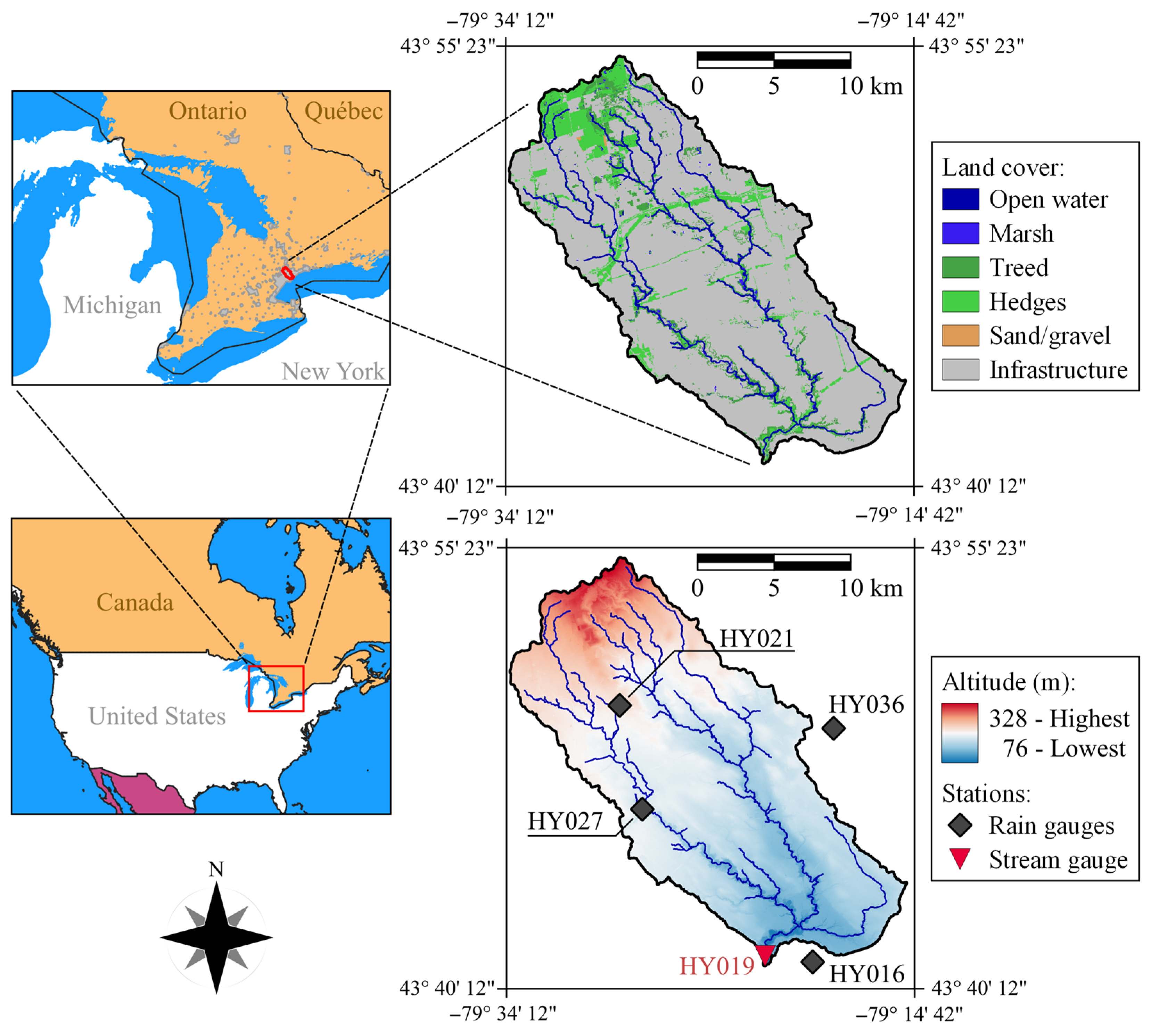
Figure 1. Location, landcover and elevations of the Don River basin with the rain and stream gauges used in this work.
Hydrology 09 00216 g001
Figure 2. Spatial granularity (before aggregation) of the data precipitation products from (a) rain gauges’ Thiessen polygons, (b) ground-based weather radar’s derived N1P product grid cells, and (c) NWM product grid cells.
Hydrology 09 00216 g002
Figure 3. Visual representation of a hypothetical ELM structure as adopted in this work. It takes two QPE products (S and Z) and antecedent discharge as input to predict the instant discharge one unit of time (hour) in the future.
Hydrology 09 00216 g003
Figure 4. Data organization scheme of the cross-folding configurations and ensemble members training setup.
Hydrology 09 00216 g004
Figure 5. Distribution of the number of nodes in the hidden layer of the ELM model selected as optimal for the different lead times.
Hydrology 09 00216 g005
Figure 6. Diagram representing the methodology for training, selecting and evaluating the ELM members of ensemble k. ε( x ) indicates the validation error of the ELM model x , nhsi indicates the i-th item in the sequence of assessed number of hidden nodes nhs., ENSk is the ensemble of models k.
Hydrology 09 00216 g006
Figure 7. Mean KGE of the models that use, besides Q t L and Q t L 1 , QPE from (a) gauges and radar, (b) gauge and CaPA, (c) radar and CaPA, and (d) all of them, including the no-QPE (None) used as benchmark.
Hydrology 09 00216 g007
Figure 8. Correlogram of the observed discharge ( Q ) variable. Violin plots represent the distribution of values across the individual rainfall-runoff events.
Hydrology 09 00216 g008
Figure 9. Taylor diagrams for the ELM models with different QPE products in their feature set at forecasting lead times ranging from 1 to 5 h (ae).
Hydrology 09 00216 g009
Figure 10. Observed hydrographs of selected events and their respective predictions at 2 h lead time.
Hydrology 09 00216 g010
Figure 11. Contingency analysis on predicting high-flow events for the ML models using only QPEs from gauge (G), only from ground-based weather radar (R), only from CaPA as representative of NWM (C), and using all of them (G,R,C).
Hydrology 09 00216 g011
Table 1. Summary of the dataset used in this work.
Original Resolution
VariableData TypeData SourceAcronymTemporal (hour)Spatial (km)
PrecipitationObservationRain gaugesG0.25Point
PrecipitationObservationWeather radarR1~2 km
PrecipitationModellingNWM (CaPA)C1~10 km
DischargeObservationRiver gaugeQ0.25Point
Table 2. Aerial representation and relative weight of each rain gauge.
Rain GaugeAerial Representativity (km2)Weight
HY01659.20.17
HY021114.90.33
HY027107.90.31
HY03666.20.19
Table 3. Summary of mean performance gains for metrics related to goodness of fit when comparing single-QPE ML models with three-QPEs ML models.
Best Single QPE3 QPEs
MetricLead Time ( h ) QPEValueValueΔ (%)
KGE1R0.940.940.00
2G0.820.842.44
3R0.630.684.76
4R0.430.5016.28
5G0.180.3172.22
RMSE   [ m 3 / s ] 1R8.448.47−0.35
2G14.6913.617.35
3R20.3719.305.25
4G25.4923.288.67
5C28.2627.074.21
r 1R0.960.960.00
2G0.870.892.30
3R0.740.774.05
4G0.560.6617.86
5C0.430.5016.28
Note: Δ(%) = 100% × (value(3 QPEs) − value(Best single QPE)) ÷ value(Best single QPE).
Table 4. Bias values of the ML models that use only one QPE and of the models that use all three QPEs for different lead times. Best values (closest to zero) for a lead time are highlighted in bold.
Lead Time (h)
Feature Set12345
G−0.06−0.10−0.17−0.22−0.22
R−0.05−0.08−0.15−0.19−0.20
C−0.07−0.13−0.18−0.23−0.22
G,R,C−0.03−0.06−0.12−0.18−0.19
Table 5. Summary of mean performance gains—metrics related to contingency analysis.
Best Single QPE3 QPEs
MetricLead Time ( h ) QPEValueValueΔ (%)
CSI1G0.720.731.38
2G0.590.58−1.69
3R0.430.454.65
4R0.300.326.67
5R0.160.1918.75
Sensitivity1G0.860.860.00
2G0.780.74−5.12
3R0.650.64−1.54
4G0.560.560.00
5G0.500.45−10.0
Precision1R0.820.831.22
2G0.700.722.86
3R0.550.597.27
4R0.380.417.89
5R0.200.2420.00
Note: Δ(%) = 100% × (value(3 QPEs) − value(Best single QPE)) ÷ value(Best single QPE).
Publisher’s Note: MDPI stays neutral with regard to jurisdictional claims in published maps and institutional affiliations.