Article

Differentiated Spatial-Temporal Flood Vulnerability and Risk Assessment in Lowland Plains in Eastern Uganda

1
Department of Environmental Management, Makerere University, Kampala P.O. Box 7062, Uganda
2
Department of Agricultural and Bio-Systems Engineering, Makerere University, Kampala P.O. Box 7062, Uganda
3
Department of Geomatics and Land Management, Makerere University, Kampala P.O. Box 7062, Uganda
4
Department of Geography, Geo-Informatics and Climatic Sciences, Makerere University, Kampala P.O. Box 7062, Uganda
*
Author to whom correspondence should be addressed.
Hydrology 2022, 9(11), 201; https://doi.org/10.3390/hydrology9110201
Submission received: 10 October 2022 / Revised: 31 October 2022 / Accepted: 1 November 2022 / Published: 9 November 2022
(This article belongs to the Special Issue Modern Developments in Flood Modelling)

Abstract

:
This study was conducted to map flood inundation areas along the Manafwa River, Eastern Uganda using HECRAS integrated with the SWAT model. The study mainly sought to evaluate the predictive capacity of SWAT by comparisons with streamflow observations and to derive, using HECRAS, the flood inundation maps. Changes in Land-use/cover showed by decrease in forest areas and wetlands, and conversions into farmlands and built-up areas from 1995 to 2017 have resulted in increased annual surface runoff, sediment yield, and water yield. Flood frequency analysis for 100-, 50-, 10-, and 5-year return periods estimated peak flows of 794, 738, 638, and 510 m3/s, respectively, and total inundated areas of 129, 111, 101, and 94 km2, respectively. Hazard classification of flood extent indicated that built-up areas and commercial farmlands are highly vulnerable, subsistence farmlands are moderately to highly vulnerable, and bushland, grassland, tropical high forest, woodland, and wetland areas are very low to moderately vulnerable to flooding. Results demonstrated the usefulness of combined modeling systems in predicting the extent of flood inundation, and the developed flood risk maps will enable the policy makers to mainstream flood hazard assessment in the planning and development process for mitigating flood hazards.

1. Introduction

In recent years, variability in natural disasters has increased due to the changes in global climate, land use/cover, and socio-economic development [1]. Statistics show that 318 natural disasters affected 122 countries worldwide in the year 2017 alone, the impacts of which resulted in 9503 deaths, 96 million people affected, and USD 314 billion as economic damages, and floods accounted for 38.3% of these disasters and 35% of deaths, affecting 59.6% of people’s livelihoods and 6.2% of economic damages [2]. Uganda, like other low-income countries, is vulnerable to extreme weather events such as droughts and floods [3]. In Eastern Uganda, the low-lying areas of Butaleja district are vulnerable to flooding [4], and more recently, in December 2019, floods led to four deaths, and over 2000 people were displaced [5].
Flood inundation mapping plays an important role in designing sustainable plans, protecting human properties and lives, and mitigating disaster risks [6]. It is also a crucial step in developing flood hazard maps and conducting proper flood assessments [7]. Flood inundation mapping usually requires repeated observations of the flooded area and inundation extents through remote sensing images [8] or ground observations [9]. Obtaining representative meteorological data for watershed-scale hydrological modeling can be difficult and time-consuming [10]. The difficulty in collecting data can be attributed to the following reasons: (i) lack of reliable equipment, (ii) absence of a good archiving system and software to store and process the data, and (iii) lack of funds to organize data collection campaigns [11]. It is also worth mentioning that once the data have been captured and archived, accessing them is quite costly [12]. Weather stations based on the ground do not always adequately represent the weather occurring over a watershed because they can have gaps in their data series and can be far from the watershed of interest or recent data are not available [13]. For data-scarce areas, hydrological and hydrodynamic models as such play a critical role in flood simulations and risk assessment [14].
Hydrologic models rely on the parameterization of watershed properties and rainfall patterns and depths to produce a flood hydrograph of discharge at discrete time steps [15]. These models have become widely used in flood forecasting, stream flow prediction, and quantifying effects of climate change and land use impacts or other spatially distributed properties. However, their limited routing methods do have some drawbacks in simulating flows in large watersheds. Examples of hydrologic modeling tools include the wflow, Hydrologic Engineering Center–Hydrologic Modeling System (HEC–HMS), the Hydrologic Simulation Program–FORTRAN (HSPF), Soil and Water Assessment Tool (SWAT), and MIKE-SHE [15]. On the other hand, hydrodynamic modeling tools are based on the solutions to St. Venant equations to calculate open channel flow. The most commonly used of these models are either one-dimensional or two-dimensional. Widely used hydrodynamic modeling tools include FLO-2d, Lisflood-FP (1D and 2D models), Water Quality Analysis Simulation Program (WASP), CE-QUALW2, Environmental Fluid Dynamics Code (EFDC), EPDRIV1, Hydrologic Engineering Center River Analysis System (HECRAS), MIKE11 (1-D model), MIKE21 (2-D model), and SOBEK [15]. The comparison between models has been a significant issue of debate in the scientific fraternity [16,17]. The resulting differences are attributed mainly to the quality of topographic and input data [18] and less to the complexity of the phenomenon itself [19]. Several studies have compared the performance of 1D and 2D hydraulic models for river flood simulations [16,20] and have concluded that all models have proven sufficiently accurate, but they still have discovered that flood inundation modeling involves several sources of uncertainty such as (1) input data (boundary and initial condition data, digital elevation models and channel bathymetry, hydraulic structures, roughness parameterization), (2) model structure (1D, 2D, quasi 2D, 1D/2D), and (3) internal model parameters. Furthermore, they emphasize the fact that no matter the quality of the input data, provided the user does not properly fit the data into the appropriate geometrical description of the model, the final results of the simulation will be of considerably lower accuracy [16].
Combining hydrodynamic models with hydrological models often compliments and overcomes the shortcomings of either type of modeling approach [21]. In the current study, the hydrologic modeling tool, namely the Soil and Water Assessment Tool (SWAT), is used to derive flow hydrographs at designated locations, which were then fed into the hydrodynamic modeling tool, namely the Hydrologic Engineering Center’s River Analysis System (HECRAS) for flood prediction. The SWAT and HECRAS programs were adopted in this study because they are freely available, user-friendly, peer-reviewed, are continuously improved and developed. The SWAT modeling system is a long-term, continuous model simulation of the watershed developed by the United States Department of Agricultural (USDA) [22]. SWAT has proven to perform well in streamflow and base-flow simulations around the world and in complex catchments with extreme events [23] since it allows the interconnections of different physical processes [24]. Additionally, the model is recognized as suitable for investigating long-term impacts, particularly in watersheds without conventional gauges [25]. HECRAS is one of the most commonly used modeling systems to analyze channel flow and floodplain delineation [26]. HECRAS uses geometric data representation as well as geometric and hydraulic computation routines for a network of natural and constructed channels of the river. HECRAS has the ability to make the calculations of water surface profiles for steady and gradually varied flow as well as for subcritical, super critical, and mixed flow regimes. HECRAS is also capable of doing modeling for sediment transport, which is notoriously difficult. The HECGeoRAS is a GIS extension with a set of procedures, tools, and utilities for the preparation of river geometry GIS data to import into HECRAS, and it is used to generate the final inundation map [27].
In recent decades, many researchers have performed flood hazard mapping in various parts of the world, as reported elsewhere [26]. Generally, basin-scale flood hazard mapping is performed worldwide [26]; however, limited research exists in the literature for Uganda river basins [28]. The main objective of this study was to analyze the inundation area along the Manafwa River network and to assess the flood hazard in the Manafwa catchment. The specific objectives pertaining to this study were to: (1) assess the land-use/cover changes, (2) evaluate the impact of LULC on the hydrologic characteristics, (3) evaluate the predictive capacity of the SWAT modeling system by comparisons with streamflow observations, and (4) derive using HECRAS the flood hazard maps. In this study, we aim to address one scientific question: (1) how suitable is the coupled hydrology-inundation model for producing probability maps of flood plain areas for mapping vulnerability and risk areas in a data-scarce area? Integrated modeling is the focus of this study because by using it to simulate the rainfall depths at different probabilities, complete flood hazard maps are obtained. Additionally, it can be used for other purposes in the design and analysis of flood mitigation measures, as well as flood forecasting and warning systems. The novelty of the present study is to combine the physically based distributed hydrologic model SWAT with the hydraulic model HEC-RAS for flood prediction in Eastern Uganda, which has not been conducted before for tropical catchments and for small watersheds. The study area is an important hydrological region in Uganda, very populous with extensive areas of rice cultivation, and no similar studies (to the authors’ knowledge) have been conducted in the past on the Manafwa Catchment. The Office of the Prime Minister (OPM) in Uganda will be in a position to strengthen the catchment planning process, and this will be a platform for further studies to be carried out on other catchments in the country.

2. Materials and Methods
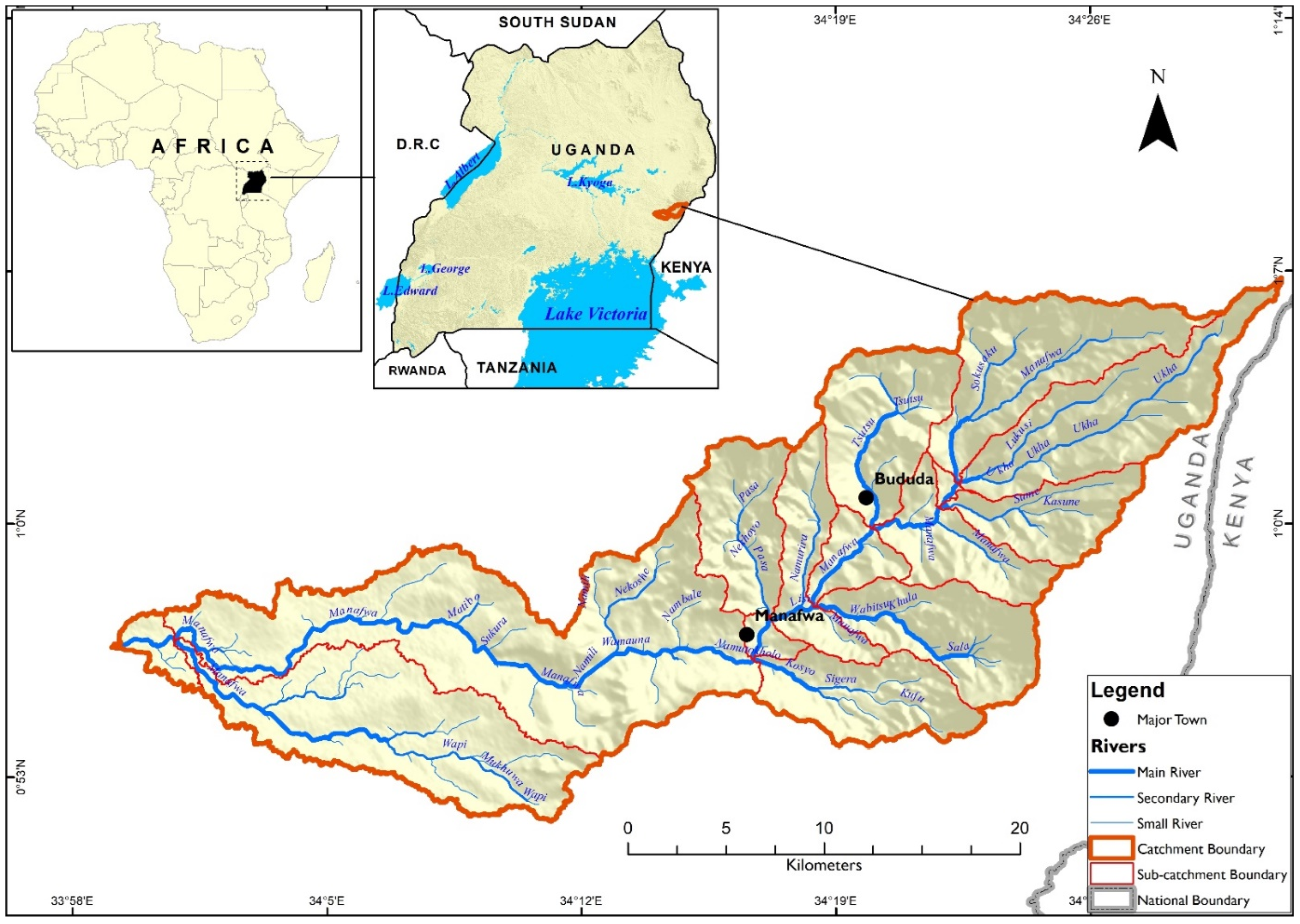
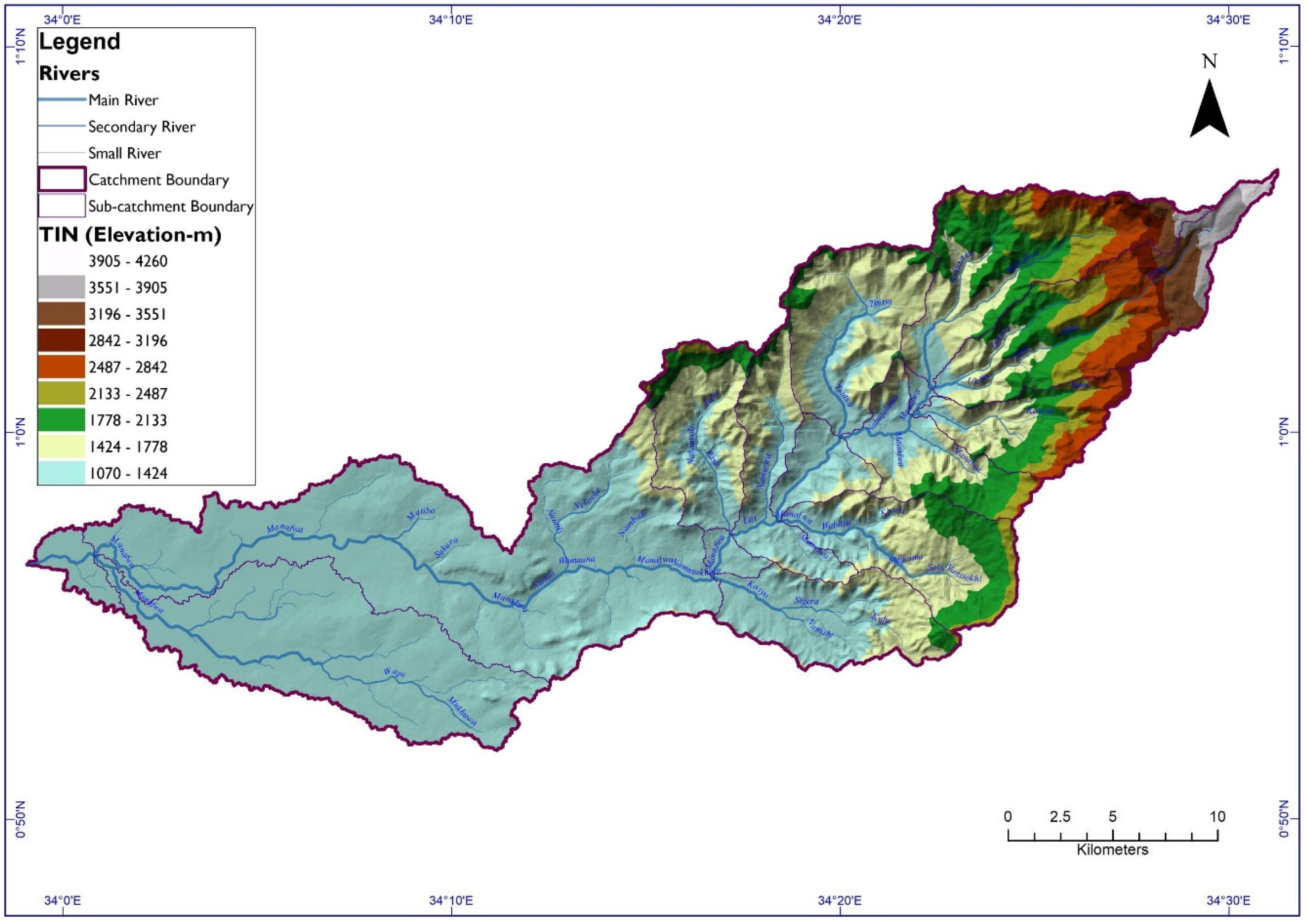
2.1. Study Area

The Manafwa catchment covers a total area of 502 km2 in the Mt Elgon region, located in the eastern region of Uganda (Figure 1). The catchment is characterized by high relief in the East, with altitudes ranging from 1041 to 4301 m above sea level, and its main stream drains from Mt Elgon to Lake Kyoga in downstream. The annual mean temperature is 23 °C, and the mean annual rainfall is 1500 mm. The annual rainfall follows a bimodal pattern, marked by the dry season covering the period of June–August (JJA) and December–February (DJF); and the rainy season occurs during the months of March to May (MAM) and short rains in September–November (SON). The geology in the Mt. Elgon region comprises mainly Pre-Cambrian and Cainozoic rock formations, including volcanics, granites, and sediments. The predominant soil type is Vertisols, regionally known as “black cotton soils”. Generally, the soils in the highlands are clays, while those in the midlands and the lowlands are clay loams or sandy. Land-use/cover changes in the catchment are characterized by the conversion from natural forest to other land-use/cover types, especially crop lands and grazing, due to the high population growth rate of 3.5% increasing demand for arable lands for crop production. The catchment is also characterized by low-income generating activities and weak infrastructural and service facilities.

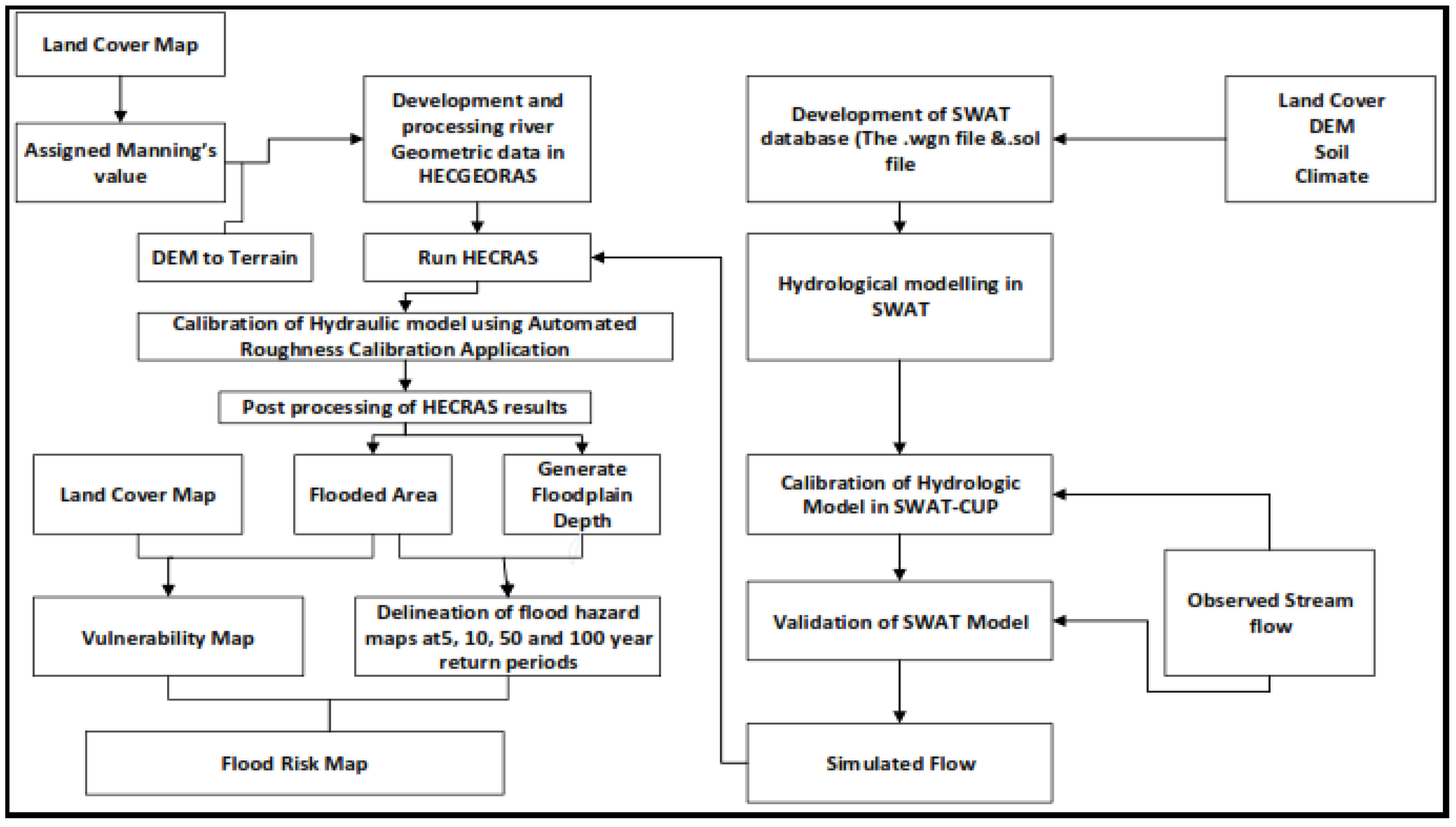
2.2. Hydrological Modelling

2.2.1. Model Input Data

In this study, the SWAT model [22] was used to simulate discharge data at the required station in the catchment for the chosen time period. A 30-m spatial resolution digital elevation model (DEM) from the Shuttle Radar Topography Mission (SRTM) downloaded from https://earthexplorer.usgs.gov/ (accessed on 10 July 2018) was used to derive the topographic information used for drainage pattern definition. A soil map was obtained from FAO, Scale- 1:50,000 (2000); Land cover maps of 1995, 2008, and 2017 (Figure 2a–c) with a spatial resolution of 30 × 30 m were obtained from National Forestry Authority (NFA), which is the mandated institution required to frequently monitor land use/cover changes in Uganda; Relative humidity, wind speed, solar radiation, and the minimum and maximum air temperatures were obtained from the Climate Forecast System Reanalysis (CFSR), which was designed based on the forecast system of the National Centers for Atmospheric Prediction (NCEP) from 1981 to 2013 https://globalweather.tamu.edu (accessed on 10 July 2018). The rain gauge network of the area is very sparse, and as such, the precipitation data were downloaded from CHIRPS for the 1981–2013 period. Daily discharge data were acquired from the Directorate of Water Resources Management, MWE for the period of 1981–2013 obtained from the Manafwa river gauge (station ID 82212)

2.2.2. Model Set-Up and Calibration

The initial model setup was carried out with the Arc SWAT 2012 (revision 664) using the DEM. A total of 19 sub-catchments were defined with 73 Hydrologic Response Units (HRUs) from a unique combination of land use/cover, soil type, and slope at thresholds over the sub-catchment area of 10% for all categories. Surface runoff and infiltration were computed using the Soil Conservation Services (SCS) curve number method. Evapotranspiration was calculated based on the Penman Monteith method using the obtained climate data (mean daily temperature, solar radiation, and wind speed). The lateral flow was calculated using a kinematic storage model described in [22]. After the initial setup, the model was calibrated and validated at a daily resolution using the Sequential Uncertainty Fitting (SUFI-2) algorithm in the SWAT Calibration and Uncertainty Program (SWAT-CUP, version 5.1.6.2) [22], following the procedures of [23]. The SUFI-2 program was applied for parameter optimization, and Latin Hypercube sampling iteratively discarded the worst simulations by rejecting the 2.5th and 97.5th percentile of the cumulative distribution. Thus, the best 95% of simulations generated a parameter range (95% prediction uncertainty, 95PPU) rather than a single final parameterization. The uncertainty band (95PPU) was used to account for the modeling uncertainty [22]. Calibration of the streamflow was performed from the year 2000 to 2010, and the validation was performed from the year 2011 to 2013.

2.2.3. Model Performance Evaluation

In this study, the model performance during calibration and validation was evaluated based on three quantitative statistics: specifically, the coefficient of determination (R2) using Equation (1), the Nash-Sutcliffe efficiency (NSE) using Equation (2), and the percent bias (PBIAS) using Equation (3). The coefficient of determination (R2) ranges between 0 and 1.0, with high values indicating less error variance. The NSE, which was used as the objective function, ranges between −∞ and 1.0. An NSE of 1.0 indicates a perfect fit between the simulated and observed data [29]. The optimal value of PBIAS is 0%, with positive and negative values indicating model underestimation and overestimation bias, respectively. The model performance was considered to be satisfactory if NSE ≥ 0.50, R2 ≥ 0.50, and PBIAS ≤ ±25% [29].
R 2 = [ i = 1 n ( O i   Ò ) ( P i ) ] 2 i = 1 n ( O i Ò ) 2   i = 1 n ( P i ) 2
N S E = 1 i = 1 n ( O i P i ) 2 i = 1 n ( O i Ò ) 2
P B I A S = 100   i = 1 n ( O i P i ) i = 1 n O i
where Oi and Pi are the measured and simulated data, respectively, Ò and are the means of measured and simulated data, and n is the number of observations. The modeling uncertainty was quantified as the P- and R-factor [22]. The P-factor measures the ability of the model to bracket the observed data with the 95PPU. The P-factor is between 0 and 1, where 1 means a 100% bracketing of the observed data. The R factor represents the width of the 95PPU, ranges from 0 to 8, and should be below 1, implying a small uncertainty band [22].

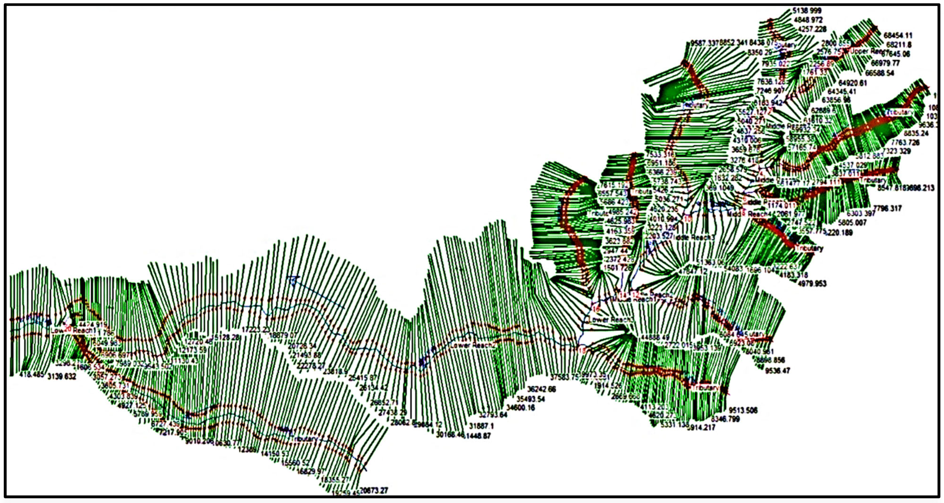
2.3. Hydraulic Modelling Using HECRAS

The hydraulic model used for our study is based on Hydraulic Engineering Center’s River Analysis System (HEC-RAS), version 5.0.3 [30]. This model was designed to perform 1D steady flow as well as 2D unsteady flow simulations for a river flow analysis and sediment transport and water temperature/quality modeling. The model uses geometric data representation as well as geometric and hydraulic computation routines for a network of natural and constructed channels of the river. The model required to discharge, DEM as a boundary condition, and Manning’s roughness coefficient derived from LULC for calibration. The Model was discretized into an equal number of grid cells of 30 m × 30 m, i.e., equal geometry to maintain spatial uniformity. HECRAS modeling within the Manafwa floodplain followed three steps (Figure 3).
Step one—This preprocessing stage involved the manual digitization of thematic vector layers (e.g., river network, stream centerline, river banks, flow paths, cross sections) in ArcGIS 10.5. software based on the STRM DEM with 30 m spatial resolution and generation of the attribute table for each of them. The DEM was used as an input in the RAS mapper of HECRAS 2D to develop a Digital Terrain Model (DTM). The DEM data were added to the New Terrain Layer dialogue of the RAS mapper in HECRAS 2D. A new terrain layer was created with terrain files that were used for evaluation. This information was saved in the terrain folder in GeoTiff format. In addition to GeoTiff, two more files were created in. hdf and. vrt formats. The file. hdf was created in the RAS mapper, which contained information on the raster data. The. vrt file helped visualize and display multiple data. For visualizing flood plain, the model geometry was coupled to DTM, and the DTM acted as a basis to create a 2D mesh using the polygon shapefile. The DEM and DTM were used for computing the water surface elevations to visualize floodplain geometry and flood risk analysis. The importance of DEM’s accuracy has been highlighted by several authors, especially in two-dimensional hydraulic–hydrodynamic modeling applications [20].
Step two (Figure 3)—This processing stage involved the import of the required parameters (e.g., Manning roughness coefficient, hydrological data) into HECRAS software to run the 2D flood simulation. Thereby, the Manning roughness coefficient (n) was calculated based on land use/cover classes in combination with typical roughness coefficient tables for each cross-section, stream centerline, and river bank intersections with values (built-up area: n = 0.3; farmland: n = 0.025; bushland: n = 0.035; tropical high forest: n = 0.1; woodland: n = 0.06; wetland: n = 0.04 [31]. Steady flow analysis was used instead of unsteady flow analysis because, in the second case, the HECRAS software needs a hydrograph, which we could not obtain from the local authorities. Thereby, to overcome this limitation, we used the flow rate for the gauging station.
Step three—This post-processing stage involved exporting the HECRAS results to the software and generating the flood patterns with the different recurrence intervals. The validation of the results was performed by comparing the real discharge recorded at the gauging station with the computed discharge hydrographs. A detailed description of HECRAS is provided by [32,33].

2.4. Flood Hazard Analysis

To assess flood hazard, the DEM was converted into Triangulated Irregular Network (TIN) format, and TIN showed that the Elevation of the study area ranged from 1070 to 4260 m (Figure 4). After that, the river cross-sections, stream centerline, stream bank lines, flow lines, and other river geometry information were extracted from the TIN for the HECGeoRAS model. The geometric data of the Manafwa River basin are shown in Figure 5. At the same time, the Manning roughness coefficient (n) was calculated based on land use/cover classes in combination with typical roughness coefficient tables for the study area [30,31]. After the RAS geometry data preparation, the HEC-GeoRAS model was used to generate the RAS GIS import file (final river geometry file) that was used as input for HECRAS.
The outputs of HECGeoRAS preprocessing provided GIS to RAS import files; thereafter, two-dimensional hydrodynamic models were created in HECRAS 5.0.3 for the flood frequency analysis of 5, 10, 50, and 100 years return periods. The Manning’s ‘n’ value, flow data, and boundary conditions were inputted in the imported GIS2RAS file, and the HECRAS results were obtained. To perform HECRAS analysis, River discharge data were used as the upstream boundary condition, while normal depth was used as the downstream boundary condition. These boundary conditions require the input of the Energy Grade Line (EGL) slope at the downstream boundary. The flow data obtained from SWAT and geometry obtained from the DEM created were also inputted. The cross-sections were created in HEC-GeoRAS. Thereafter, the water surface profiles were obtained, and the sufficiency of cross-section coverage was checked. River cross-sections were used at 100 m distance each, and 500 cross-sections were generated for the analysis. The 1D model was connected to the floodplain, and a 2D computational mesh was created at 100 × 100 m grid size. Although the cell size is rather large, considerable hydraulic details are still retained within a cell using the 2D Geometric Preprocessor. The algorithm preprocesses cells and cell faces to develop detailed hydraulic property tables (elevation versus wetted perimeter, elevation versus area, roughness, etc.) based on the underlying terrain (5 × 5 m in this case). As such, HEC-RAS can produce detailed results (for example, a cell can be partially wet), which is an advantage over other models that use a single elevation for each cell [30]. The outputs were exported to GIS from HECRAS, and water surface TINs were created in the Arc GIS environment. Thereafter, flood plain extent and depth grids were obtained, and flood hazard maps for 5-, 10-, 50-, and 100-year return periods were prepared using Arc GIS.
A flood hazard assessment was undertaken based on the flood water depth indicated by the prepared flood map of the Manafwa watershed. For this, hazard levels were ranked in terms of water depth, and these levels were determined by reclassifying the flood grid water depth bounding cells. Five hazard levels were categorized based on water depth such as very low (<0.5 m), low (0.5–1 m), moderate (1–1.5 m), and high (1.5–2 m) and very high (>2 m) area bounded by each level calculated by modification of the scale used in the MLIT methodology [34] and flood hazard maps were prepared.

2.5. Flood Vulnerability Analysis

The first step in vulnerability analysis was to identify the elements at risk in the study area. In this study, elements at risk were identified by overlying the land-use/cover onto flood inundation maps. LULC dataset was generated from the digital image classification of Landsat, satellite images of 1995, 2008, and 2017 with a spatial resolution of 30 × 30 m, downloaded from Global Land Cover Facility (https://glovis.usgs.gov/) (accessed 10 July 2018 (Table 1). Images from the same period (March–May), i.e., the first rainy season, were selected in order to minimize the seasonal effect on the classification results. In this study, supervised classification of the maximum likelihood algorithm was applied to classify Landsat images into discrete LULC categories. The area was classified into the following land-use/cover classes: built-up areas, bushlands, grassland, commercial farmland, subsistence farmland, tropical high forest, woodland, and wetland. Information collected during the field survey as ground-truthing point was used to assess the accuracy of classification. The elements at risk identified for the study areas included commercial farmland, subsistence farmland, and rural settlements (i.e., homesteads) because other land-use/cover classes were not important from a flood risk point of view. Finally, inundation layers were overlaid on the land-use/cover layer to obtain the overlaid zones. From the ArcGIS overlay analysis, different sorts of inundation statistics were generated. The land-use/cover areas under the influence of each flooding event were reclassified for the calculation of the total vulnerable areas.

2.6. Flood Risk Analysis

The flood risk analysis included the combination of the results of both the vulnerability analysis and the hazard analysis by intersecting the flood depth polygons prepared during the hazard analysis with the land-use/cover vulnerability polygons. The resulting attribute tables were reclassified to develop the land-use/cover-flood depth relationship. Potential flood areas in terms of both the land cover vulnerability classes and water depth hazard classes were then presented. Flood risk maps were then prepared by overlaying the flood depth grids with the land-use/cover map. The following equation was used to generate the flood risk map of the Manafwa catchment in the raster calculator of ArcGIS. Finally, and based on Equation (4), flood risk was reclassified into five classes, as shown in Table 2
Risk Map = Hazard Map × Vulnerability Map

3. Results

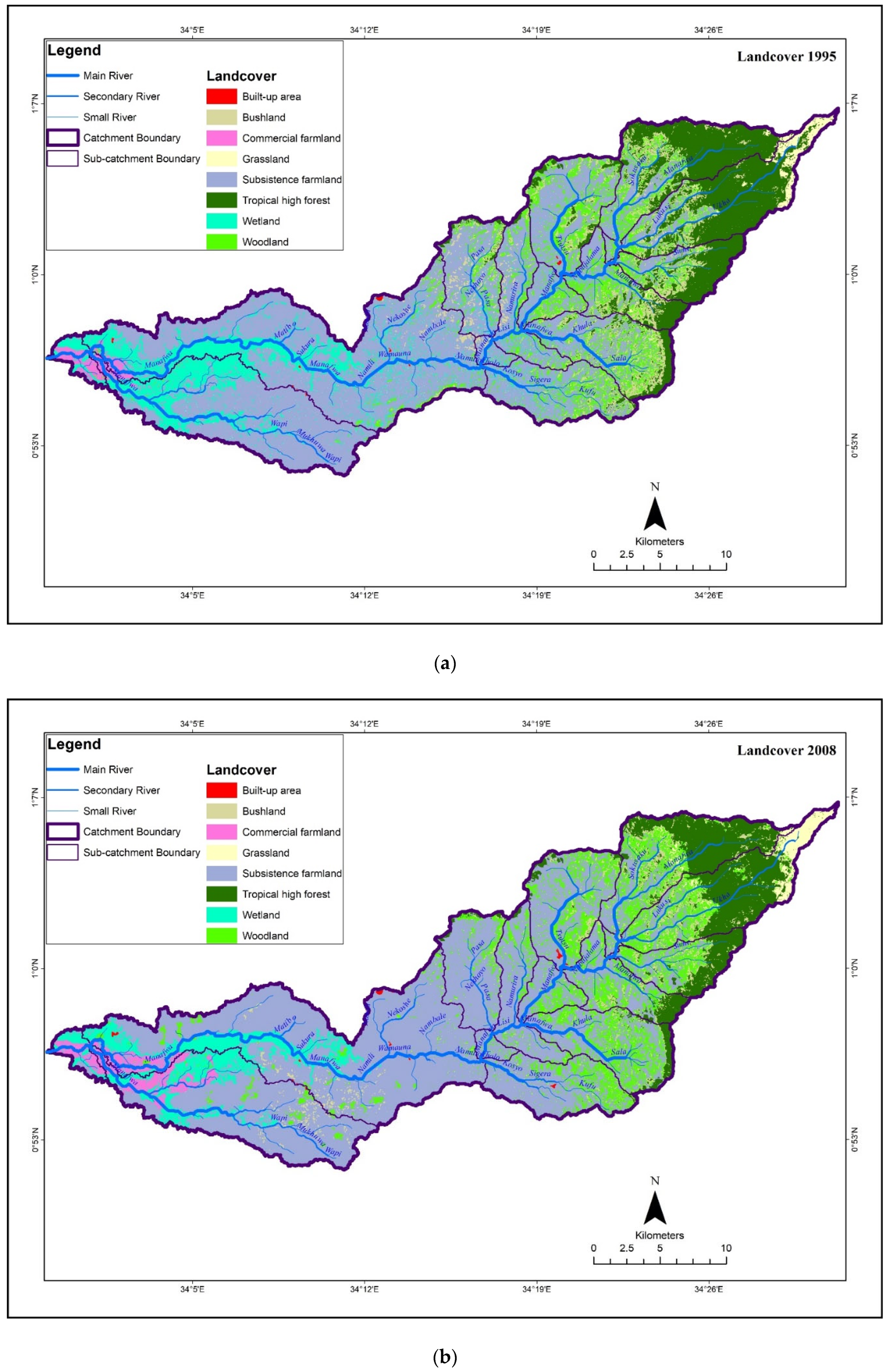
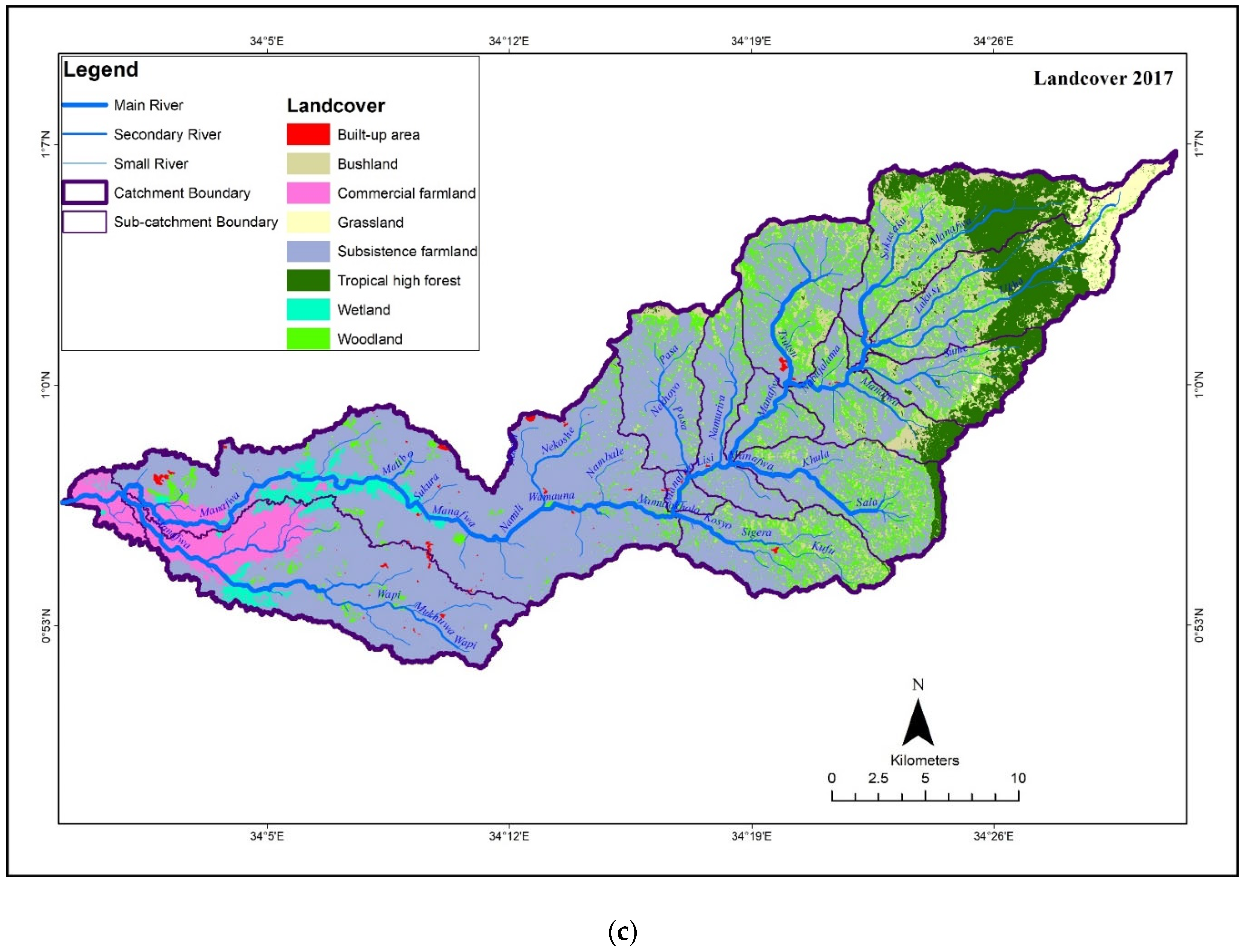
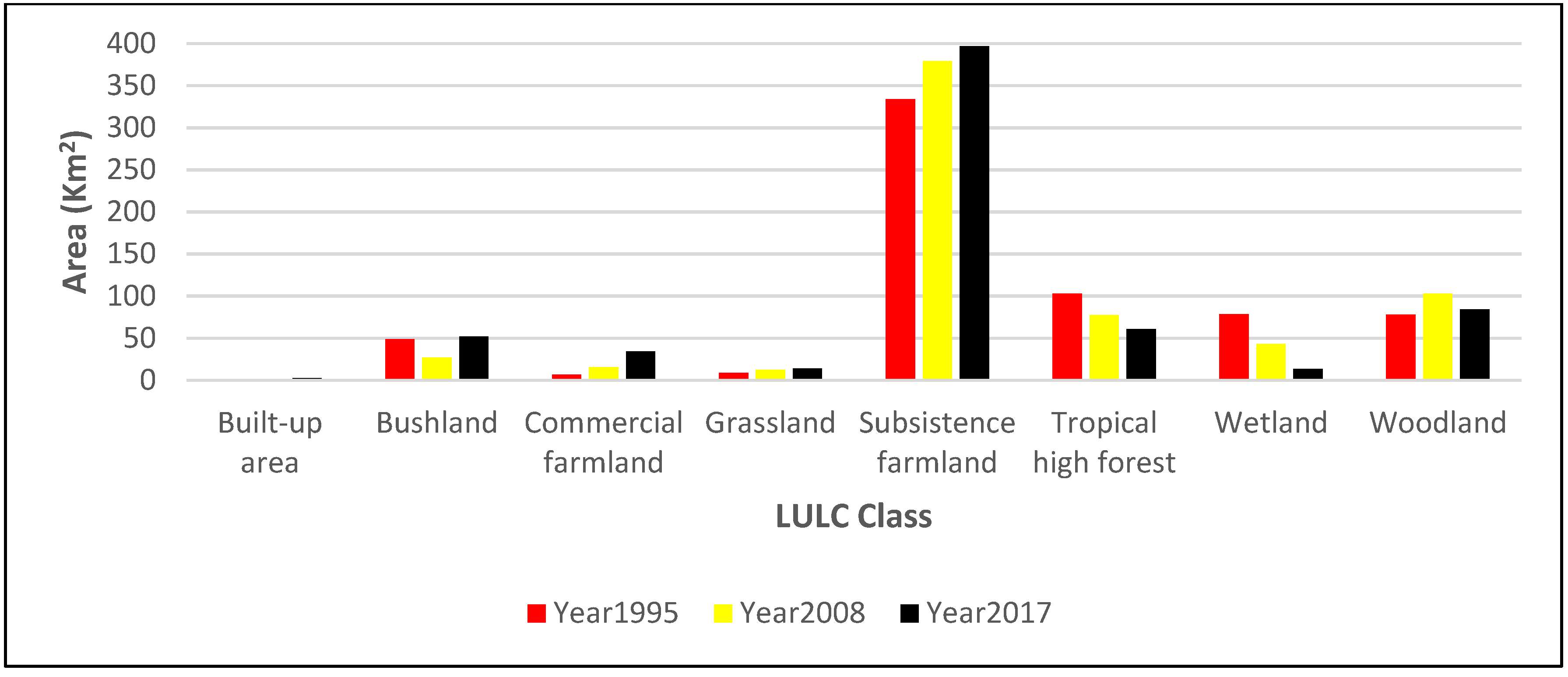
3.1. Land Cover Classification in Manafwa Catchment

There are eight land-use/cover types identified in the Manafwa catchment, which are built-up area, bushland, commercial farmland, grassland, subsistence farmland, tropical high forest, wetland, and woodland (Figure 6). Subsistence farmland, Tropical High forest, wetland, and woodland were the dominant LULC types at the beginning of the study period (Figure 6). However, bushland, wetland, and tropical high forests significantly declined whilst subsistence farmland, commercial farmland, and woodland increased during the 1995–2008 period. The period of 2008–2017 is characterized by an increase in bushland, commercial farmland, and subsistence farmland with a marked decrease in the tropical high forest, wetland, and woodland.

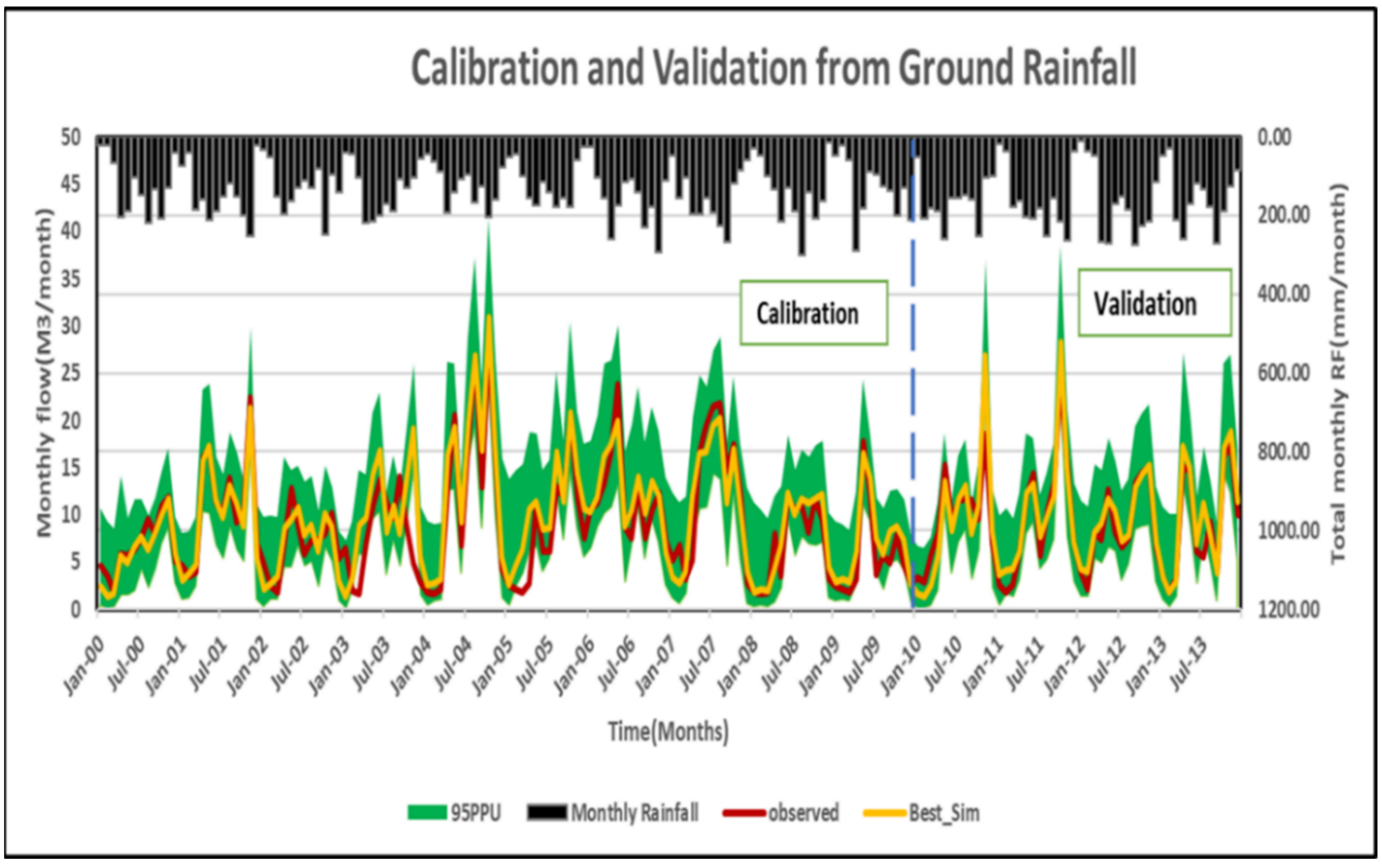
3.2. Model Calibration, Sensitivity, and Uncertainty Analysis

Through the sensitivity analysis of the SWAT model, 14 parameters with higher sensitivity were selected to calibrate and verify the model (Table 3). Sensitivity was evaluated based on t-stat values (a higher absolute value is more sensitive). Significance was also determined based on the p-value. Sequential Uncertainty Fitting program (SUFI-2) flow calibration was performed for the simulated results based on the sensitive parameters. This was conducted by simulating the flow for 26-year period, including two-year warm period from 1981–2013. The values of NSE and R2 (Table 4) after calibration are greater than 0.65, which is the best predictor of the model. After calibrating (2000–2010) and obtaining acceptable values of NSE and R2, validation of simulated stream flow for 3-year period, including one-year warm-up period from 2011 to 2013, was performed using monthly observed flows. The results after validation were also checked using NSE and R2 and had magnitudes greater than 0.65 and 0.77, respectively, for the 2008 and 2017 (Table 5), except for 1995, which has an NSE value less than 1. The PBIAS also shows a good estimation since the values are less than ±25%, except for 1995. The calibrated and validated stream flow results showed a good agreement with the observed data (Table 4 and Figure 7) and therefore indicate that the SWAT model is a good predictor of stream flow of the Manafwa watershed.

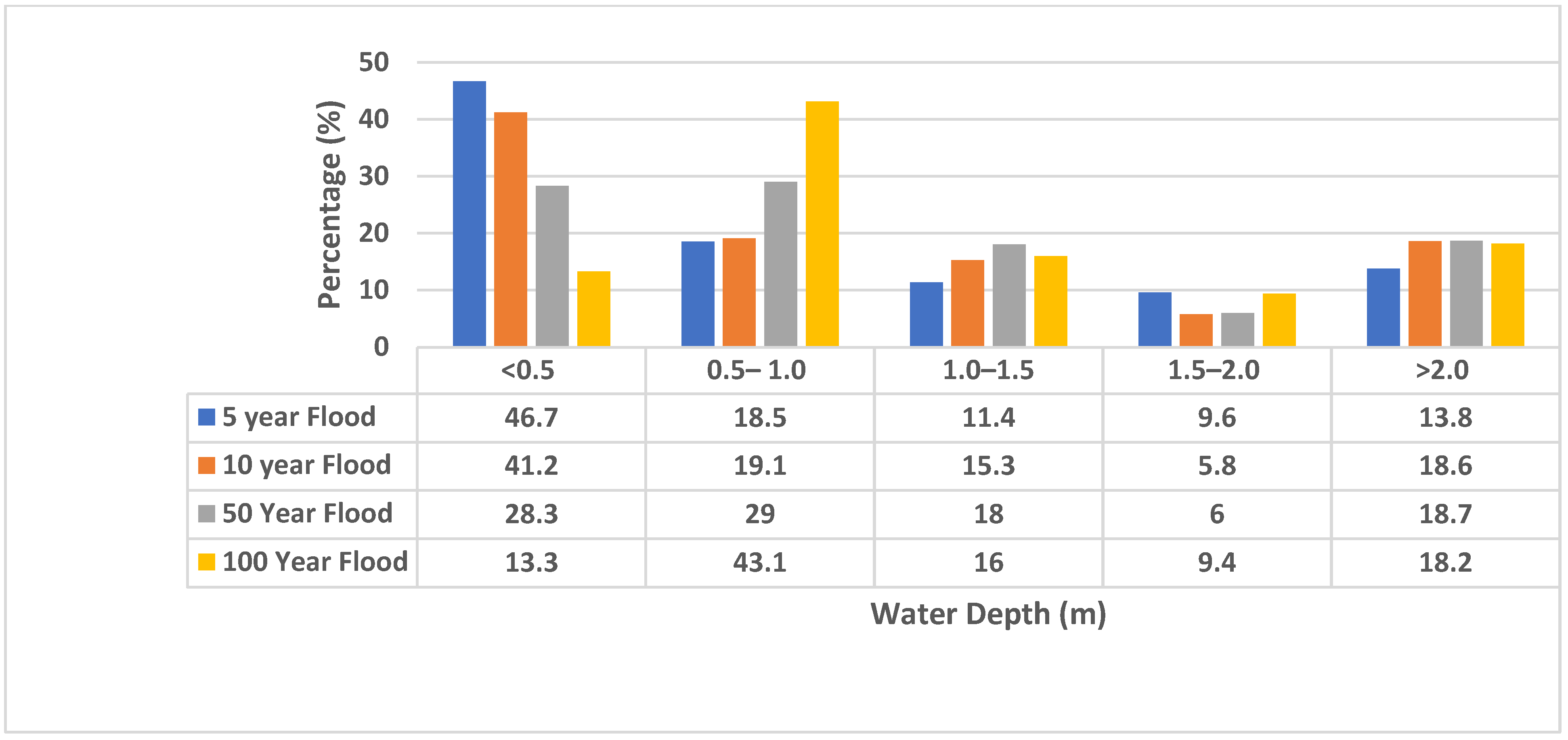
3.3. Inundation Areas Mapped

The analysis of flood inundation area indicated that a considerable increase in flood inundation with increasing discharge of flood was shown from 5 years to 100 years return period (Figure 8). The classification of flood depth areas indicated that 13–19% of the total flooded areas had water depths greater than 2 m.

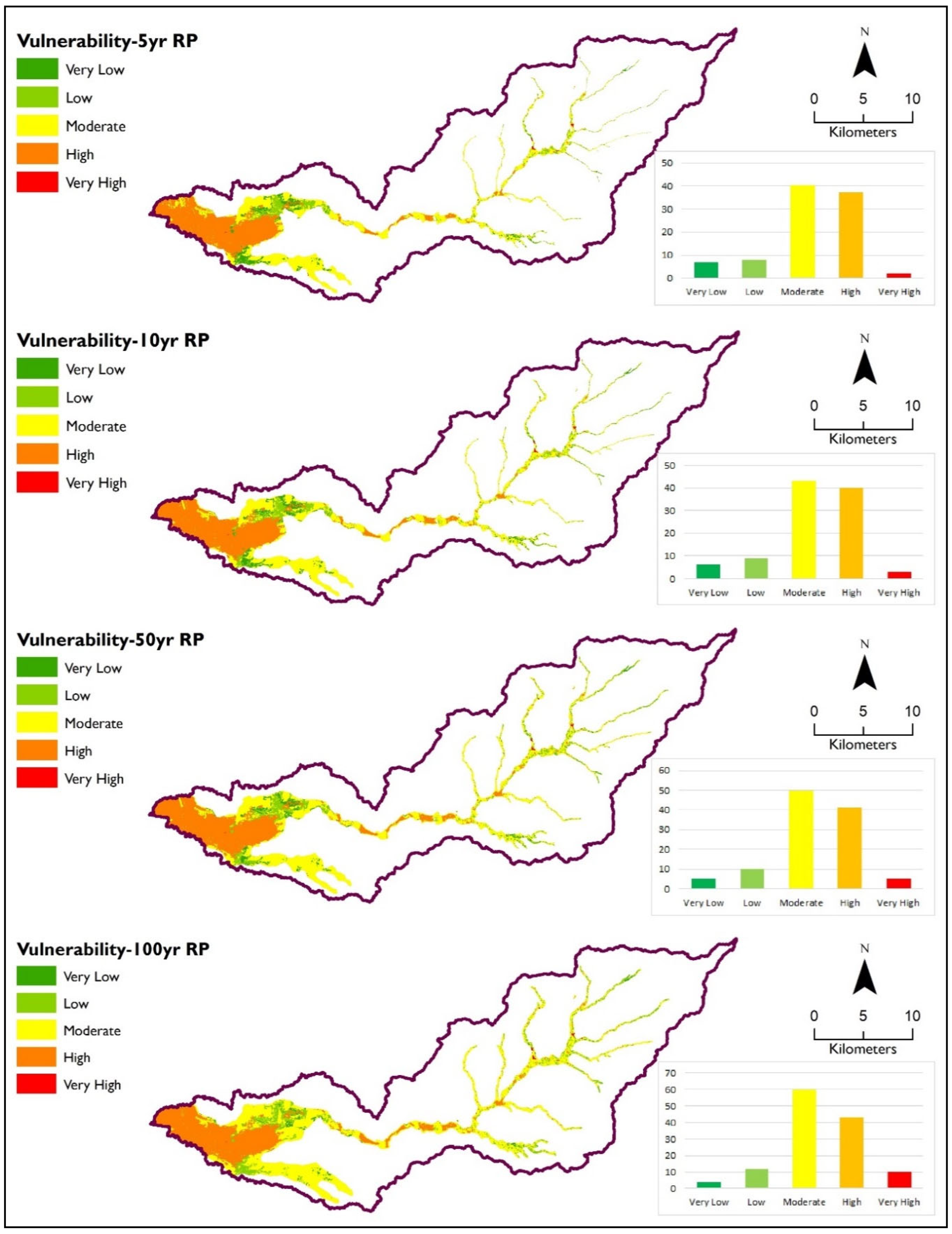
3.4. Floodplain Vulnerability

The land cover area under the influence of modeled flood showed that 42.7, 33.7, 10.8, and 5.3 km2 of subsistence farming area, forest commercial farming area, wetland, and woodland area are respectively inundated by 5-year flood, and the total vulnerable area is 94 km2 (Figure 9). The very high flood vulnerability areas covered 12.9 km2, and high vulnerability areas occupied 9.0 km2. Moderate, low, and very low vulnerability zones were 10.7, 17.4, and 43.9 km2, respectively. Similarly, 67.9, 34.2, 12.3, and 9.7 km2 of subsistence farming area, forest commercial farming area, wetland, and woodland area were respectively inundated by a 100-year flood, which showed flooded areas increased with an increase in flooding intensity; mostly subsistence farming area was inundated by different year floods, which was followed by commercial farming and wetland area. The flood vulnerability results for the 100 Yr. return period showed that the total vulnerable area is 128.7 km2. The very high flood vulnerability areas covered 23.4 km2, high vulnerability areas occupied 12.1 km2, while moderate, low, and very low vulnerability zones were 20.6, 55.6, and 17.1 km2, respectively.
According to [35], integrated flood management and land cover change, along with HECRAS hydraulic model simulations, are required for flood risk mitigation. Therefore, land cover change in the Manafwa basin was analyzed in two time periods, and the comparisons for the different two time periods shows that flooded area in Commercial farming, subsistence farming, Bushland, and Woodland has increased, but flooded areas in Wetland and Tropical High Forest decreased (Table 5).

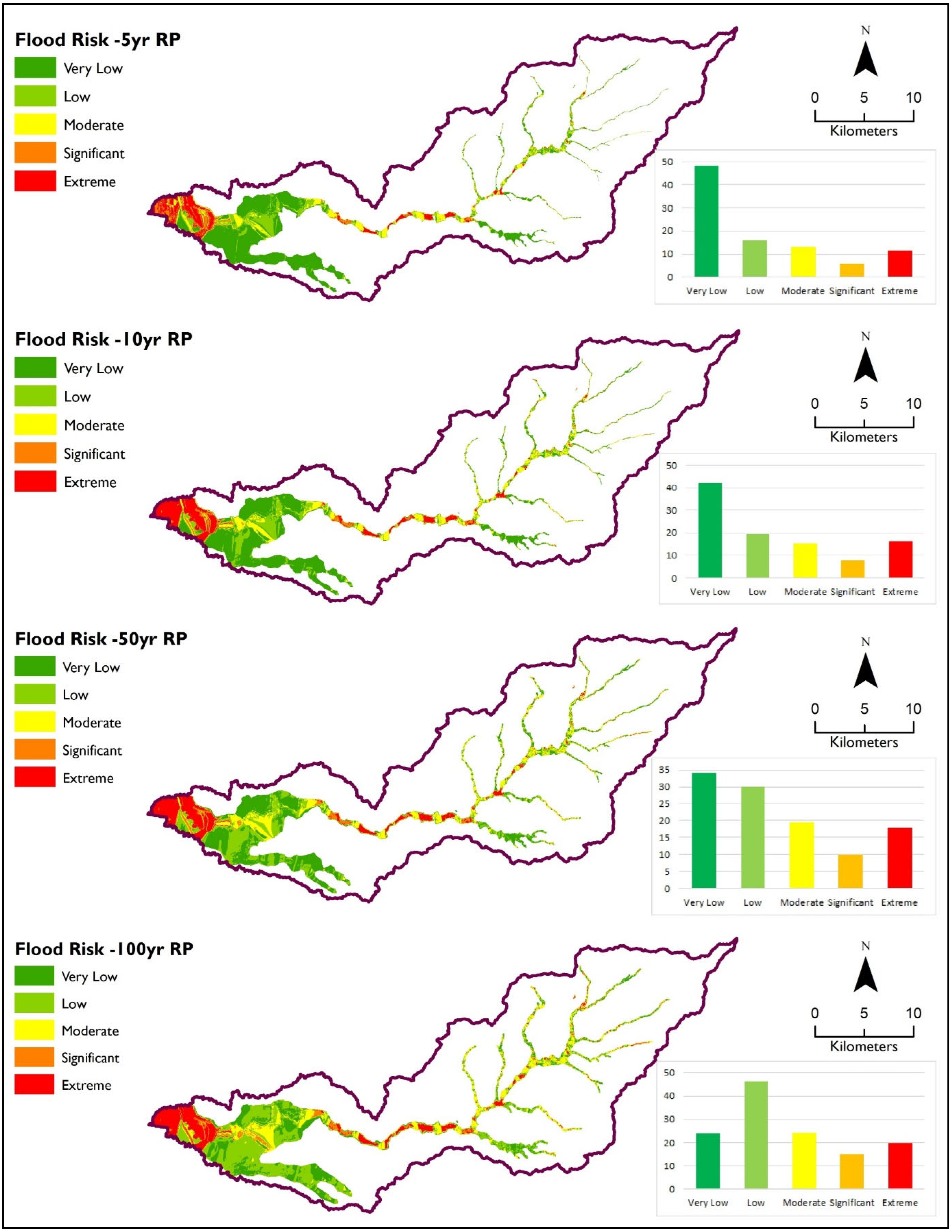
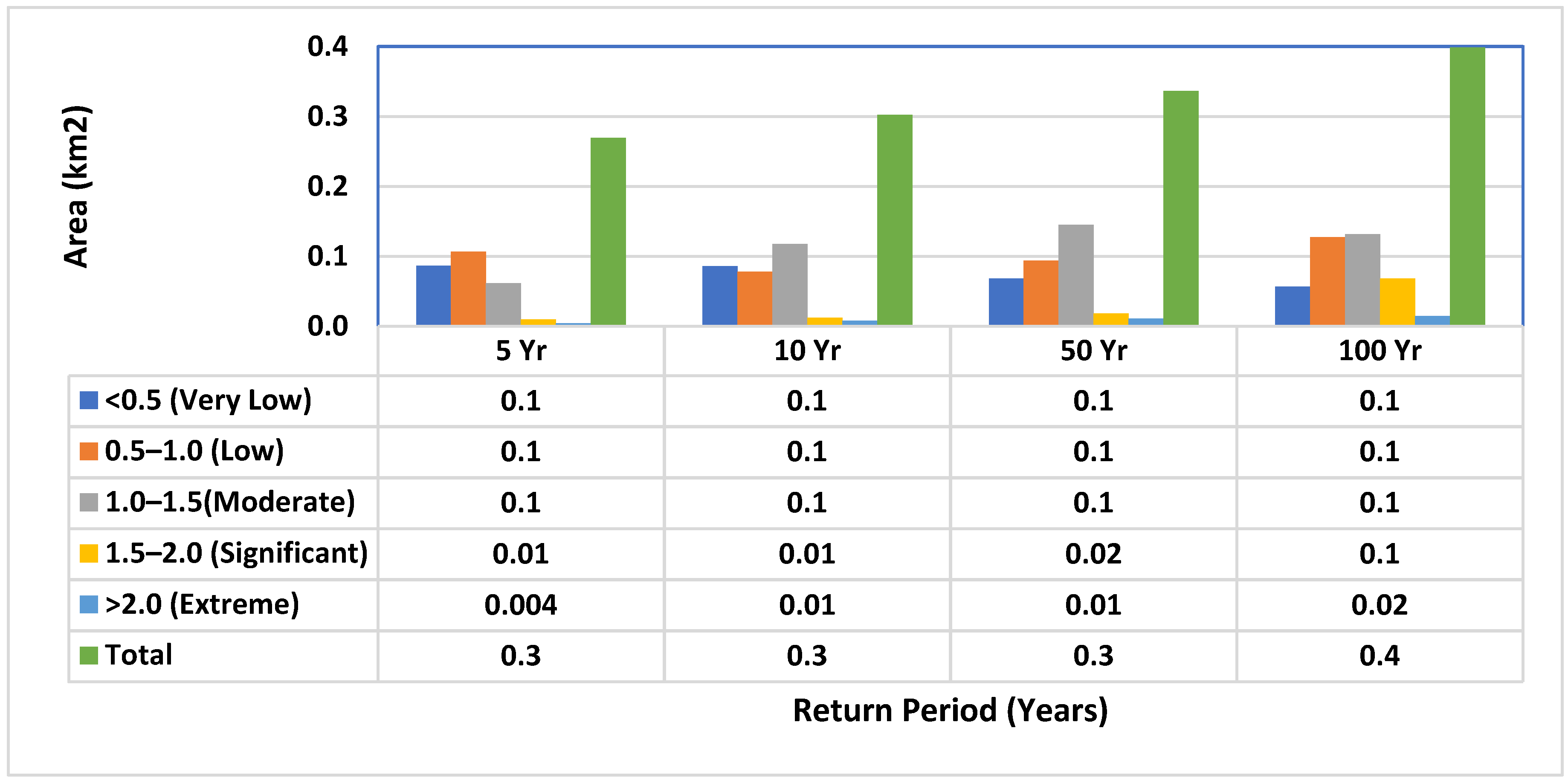
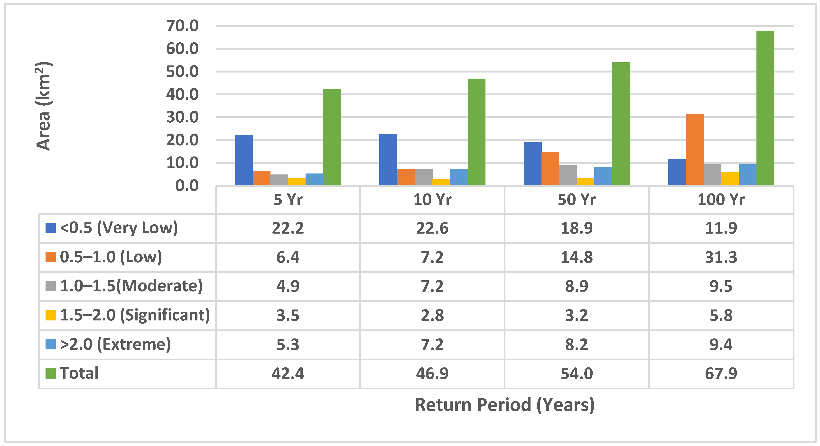
3.5. Flood Risk Analysis

The classification of risk for the 5 YR and 100 YR return periods showed that commercial farmland, subsistence farmland, and Built-up/Settlement areas were under extreme risk of floods (Figure 10). The extreme flood risk areas covered 11.3 km2; significant risk areas occupied 5.7 km2, while moderate, low, and very low-risk zones were 12.9, 15.9, and 48.2 km2, respectively. Similarly, for the 100 YR return period, the extreme flood risk areas covered 20.0 km2, and significant flood risk areas occupied 15.0 km2. Moderate, low, and very low-risk areas were 24.0, 46.0, and 23.7 km2, respectively.
The analysis of the relationship between the flood hazard level and settlement area (Figure 11) indicated a gradual increase in the significant and extreme hazard classes in all return periods. There is no change in the very low, low, and moderate hazard classes in all return periods.
Similarly, Subsistence farming area under a very low hazard class (<0.5 m) is 22.2, 22.6, 18.9, and 11.9 km2 for return periods of 5–100 years (Figure 12). It also shows that there is a gradual increase in the low, moderate, and extreme hazard classes.
In the commercial farming land cover type, there is a gradual increase in every return period in the low, moderate, and extreme hazards and a gradual decrease in every return period in the very low hazard (Figure 13).

4. Discussion

SWAT is one of the most widely used models when simulating water balance within a basin [36]. However, the software has some limitations related mostly to a large number of input parameters. Sometimes, several parameters must be obtained or estimated from global databases, equations, or other computer software [37]. The information gave a satisfactory representation of the total flow behavior in the basin once the model was calibrated for the different land coverage scenarios. The error metrics for calibration and validation periods in the Manafwa catchment were “good”, according to [29]. Ref [29] recommended that the general performance of objective functions on monthly time step calibration are satisfactory if NSE > 0.50 and RSR ≤ 0.70, and if PBIAS ≤ ±25% for streamflow.
The combination of Arc GIS and HECRAS 2-D flood simulation model indicates the capability of simulating flood events and spatially depicting the degree of exposure or vulnerability of the region towards a hazard event in terms of inundation extent and depth of water levels. The model can be said to have generated reliable quantified output. This hybrid approach provides quantified information on the water level depths and facilitates access to the data at any point of interest. As there are no quantified data on the inundation depths for flood hazards in the study region, the visualization and the quantification of the flood risks, as facilitated by this approach, can generate invaluable information and assist the decision-making authorities to making informed choices towards mitigating the catastrophic effects of flooding disasters.
Whereas in literature, there is considerable debate about whether a 1D or a 2D model provides a better representation of a flood event [21], it should be noted that even for the most sophisticated models, the performance of models is influenced by the quality of the source of information that is available for their parameterization, calibration, and validation. This is especially critical in undeveloped countries where financial and data sources are scarce. With regard to the calibration or validation of the model result, it could have been improved if it had been possible to compare it to an actual flood event, e.g., upstream and downstream flow hydrographs, mapped and recorded inundation extents, depths, or flow velocities. Such data were not available for the model area.
The lack of appropriate infrastructures and data makes the development of FHA difficult in African countries beyond the inclusion of this continent in global risk studies, such as those cited in [38]. In most African countries, the 30 m spatial resolution digital elevation model (DEM) from the SRTM project or the ASTER project, or the SRTM-derived ‘Bare-Earth’ DEM and Multi-Error-Removed Improved-Terrain (MERIT) DEM are the best options. The lack of detailed DEMs can be considered as one but not the only key factor of the limited FHA in Africa. Apart from the lack of DEMs for flood hazard analysis, the poor quality or limited availability of flow data must be kept in mind [39].
The vulnerability assessment approach used in this study for identifying and providing a vulnerability rank based on land use/cover in the flood area is a simple yet powerful approach. It not only identified the most to least vulnerable critical land-use/cover types but also provided enough information for flood preparedness processes that could significantly reduce the impact. The approach could easily be extended for the vulnerability evaluation of other infrastructures in order to estimate economic losses, the navigation route of people, including high-density areas, and other region-specific important factors. Moreover, futuristic higher magnitude flood events can be simulated to assess magnified vulnerability and associated risks. Land use planning decisions could be made based on flood inundation maps. Following such approaches will help save lives and resources at the same time and provide a proven and more accurate way to contest the uncertainties of the natural events causing floods.
It should be kept in mind that uncertainties exist in every stage of flood hazard mapping, from the beginning of the process (data collection, model selection, parameter selection, input data, model calibration, operation, and handling of the models) until the outcome is obtained [40]. The main limitations of this study were data quality and availability (e.g., missing rainfall and hydrologic data; unevenly distributed discharge and water level gauges with varying time series length and missing data; little field survey cross-section data and lack of hydraulic structure data along the river, such as bridges, weirs, etc.) contributing to uncertainties and inaccuracy in the results. The accuracy of the flood maps could be improved through the identification of possible sources of uncertainty and uncertainty analysis; the sources of uncertainty include the DEM resolution. The current 30 m is not sufficient and could lead to errors. We, therefore, recommended this for further research, as well as the integration of better-quality data into the models if they become available.

5. Conclusions

This study presented a systematic approach of coupling the hydrodynamic model HEC-RAS with the hydrologic model SWAT in delineating flood inundation zones and subsequently assessing the vulnerability of different land cover types in the Manafwa River Watershed Eastern Uganda. The HEC-RAS flood simulation model was found to be capable of simulating flood events and spatially depicting the vulnerability of the region towards a hazard event in terms of inundation extent, whereas SWAT was proven to be an appropriate tool in generating simulated flood hydrographs at desired locations. The calibration and validation results of the streamflow generally show good agreement with the observations in terms of R2, PBIAS, and Nash-Sutcliffe efficiency coefficient. This study demonstrates a useful case study for applying the coupled hydrological and hydraulic models for flood hazard mapping. The integrated model used in this study could also be used for the analysis and design of possible structural measures and alternatives or be improved to establish a flood forecasting and warning system. The real-time inundation maps generated from forecasting systems are also an effective tool to inform relevant stakeholders and can significantly assist in communication with residents in areas susceptible to flooding. In the future, additional river survey data and high-resolution satellite images should be used for calibrating the model and improving the accuracy of flood hazard mapping. More hydro-meteorological observation stations are advocated to be installed in Manafwa and its surrounding area to provide first-hand hydrological information.
The results of the paper can be applied, especially in the areas of prevention, flood risk management, and crisis management. By incorporating flood maps into the local development plan of the catchment area, irresponsible expansion and densification of construction near the watercourse or in areas with moderate and high degrees of flood hazard could be prevented. In general, it is concluded that the use of integrated models to develop probabilistic flood hazard maps is an important step in the future flood protection of the Manafwa River Basin and similar river systems in Uganda and in the region. From the methodological point of view, the importance of the paper can be seen in the universality of the proposed steps to assess flood hazard and flood risk, which could be transferred to other similar flood-prone areas. However, further case studies in other regions should be undertaken to verify their general applicability. There are several potential research directions that can be mentioned as the next step, such as the comparison of HECRAS results with other 2D models such as Iber and BASEMENT. All three models are free, and such a comparison will highlight the advantages and disadvantages of each model’s structure as well as the assumptions for the applied location.

Author Contributions

Conceptualization, G.E., I.K., A.G. and Y.B.; data curation, G.E.; formal analysis, G.E. and I.K.; funding acquisition, Y.B.; Investigation, G.E.; methodology, G.E. and I.K.; software, G.E.; supervision, A.G., Y.B., A.E. and I.K.; writing—original draft, G.E.; writing—review and editing, G.E., I.K., A.G., Y.B. and A.E. All authors contributed to the writing of the manuscript. All authors have read and agreed to the published version of the manuscript.

Funding

This research was funded by Swedish International Development Agency (SIDA) under the Building Resilient Ecosystems and Livelihoods to Climate Change and Disaster Risks (BREAD) project (Project, 331).

Institutional Review Board Statement

Not applicable.

Data Availability Statement

Not applicable.

Acknowledgments

The authors are grateful to the Ministry of Water and Environment for providing the hydrological data that were used for the simulation of the hydrological model. Further, the authors also extend gratitude to Nsiimire Peter for his contribution to field data collection.

Conflicts of Interest

The authors declare no conflict of interest. The funding sponsors had no role in the design of the study; in the collection, analyses, or interpretation of data; in the writing of the manuscript, and in the decision to publish the results.

References

  1. Arnell, N.W.; Gosling, S.N. The Impacts of Climate Change on River Flood Risk at the Global Scale. Clim. Chang. 2016, 134, 387–401. [Google Scholar] [CrossRef] [Green Version]
  2. Cred Crunch. Natural Disasters in 2017: Lower Mortality, Higher Cost; Technical Report; Centre for Research on the Epidemiology of Disasters: Brussels, Belgium, 2018; pp. 1–2. [Google Scholar]
  3. Mubialiwo, A.; Onyutha, C.; Abebe, A. Historical rainfall and evapotranspiration changes over Mpologoma catchment in Uganda. Adv. Meteorol. 2020, 2020, 8870935. [Google Scholar] [CrossRef]
  4. Ministry of Water and Environment. Mpologoma Catchment Management Plan; Ministry of Water and Environment: Kampala, Uganda, 2018.
  5. Floodlist. Uganda—Deadly Floods and Landslides in Eastern Region (Updated). 2020. Available online: https://floodlist.com/africa/uganda-floods-bududa-sironko-december-2019 (accessed on 5 February 2021).
  6. Pinos, J.; Timbe, L. Performance assessment of two-dimensional hydraulic models for generation of flood inundation maps in mountain river basins. Water Sci. Eng. 2019, 12, 11–18. [Google Scholar] [CrossRef]
  7. Vojtek, M.; Vojteková, J. Flood hazard and flood risk assessment at the local spatial scale: A case study. Geomat. Nat. Hazards Risk 2016, 7, 1973–1992. [Google Scholar] [CrossRef] [Green Version]
  8. Alahacoon, N.; Matheswaran, K.; Pani, P.; Amarnath, G.A. Decadal Historical Satellite Data and Rainfall Trend Analysis (2001–2016) for Flood Hazard Mapping in Sri Lanka. Remote Sens. 2018, 10, 448. [Google Scholar] [CrossRef] [Green Version]
  9. Cao, C.; Xu, P.H.; Wang, Y.H.; Chen, J.P.; Zheng, L.J.; Niu, C.C. Flash Flood Hazard Susceptibility Mapping Using Frequency Ratio and Statistical Index Methods in Coalmine Subsidence Areas. Sustainability 2016, 8, 948. [Google Scholar] [CrossRef] [Green Version]
  10. Nkiaka, E.; Nawaz, N.; Jon, C. Evaluating global reanalysis datasets as input for hydrological modelling in the Sudano-Sahel Region. J. Hydrol. 2017, 4, 13. [Google Scholar] [CrossRef] [Green Version]
  11. Gorgoglione, A.; Gioia, A.; Iacobellis, V.; Piccinni, A.; Ranieri, E. A rationale for pollutograph evaluation in ungauged areas, using daily rainfall patterns: Case studies of the Apulian Region in Southern Italy. Appl. Environ. Soil Sci. 2016, 2016, 9327614. [Google Scholar] [CrossRef] [Green Version]
  12. Liu, G.; He, Z.; Luan, Z.; Qi, S. Intercomparison of a lumped model and a distributed model for streamflow simulation in the Naoli River Watershed, Northeast China. Water 2018, 10, 1004. [Google Scholar] [CrossRef] [Green Version]
  13. Daniel, R.; Todd, M.; Charlotte, M.; Arthur, T.; Zachary, M.E. Using the Climate Forecast System Reanalysis as Weather Input Data for Watershed Models. Hydrol. Process. 2014, 28, 5613–5623. [Google Scholar] [CrossRef]
  14. Yu, Y.H.; Zhang, H.B.; Singh, V.P. Forward Prediction of Runoff Data in Data-Scarce Basins with an Improved Ensemble Empirical Mode Decomposition (EEMD) Model. Water 2018, 10, 388. [Google Scholar] [CrossRef] [Green Version]
  15. Chomba, I.C.; Banda, K.E.; Winsemius, H.C.; Chomba, M.J.; Mataa, M.; Ngwenya, V.; Sichingabula, H.M.; Nyambe, I.A.; Ellender, B. A Review of Coupled Hydrologic-Hydraulic Models for Floodplain Assessments in Africa: Opportunities and Challenges for Floodplain Wetland Management. Hydrology 2021, 8, 44. [Google Scholar] [CrossRef]
  16. Horrit, M.S.; Bates, P.D. Evaluation of 1D and 2D numerical models for predicting river flood inundation. J. Hydrol. 2002, 268, 87–99. [Google Scholar] [CrossRef]
  17. Neal, J.C.; Fewtrell, T.J.; Bates, P.D.; Wright, N.G. A comparison of three parallelisation methods for 2D flood inundation models. Environ. Model. Soft. 2009, 25, 398–411. [Google Scholar] [CrossRef]
  18. Cook, A.; Merwade, V. Effect of topographic data, geometric configuration and modeling approach on flood inundation mapping. J. Hydrol. 2009, 377, 131–142. [Google Scholar] [CrossRef]
  19. Neal, J.C.; Villanueva, I.; Wright, N.; Willis, T.; Fewtrell, T.; Bates, P.D. How much physical complexity is needed to model flood inundation? Hydrol. Process. 2012, 26, 2264–2282. [Google Scholar] [CrossRef] [Green Version]
  20. Papaioannou, G.; Loukas, A.; Vasiliades, L.; Aronica, G.T. Flood inundation mapping sensitivity to riverine spatial resolution and modelling approach. Nat. Hazards. 2016, 83, 117–132. [Google Scholar] [CrossRef]
  21. Jha, M.K.; Afreen, S. Flooding Urban Landscapes: Analysis Using Combined Hydrodynamic and Hydrologic Modeling Approaches. Water 2020, 12, 1986. [Google Scholar] [CrossRef]
  22. Arnold, J.G.; Moriasi, D.N.; Gassman, P.W.; Abbaspour, K.C.; White, M.J.; Srinivasan, R.; Santhi, C.; Harmel, R.D.; van Griensven, A.; van Liew, M.W.; et al. SWAT: Model use, calibration, and validation. Trans. ASABE 2012, 55, 1491–1508. [Google Scholar] [CrossRef]
  23. Abbaspour, K.C.; Rouholahnejad, E.; Vaghefi, S.; Srinivasan, R.; Yang, H.; Kløve, B. A continental-scale hydrology and water quality model for Europe: Calibration and uncertainty of a high-resolution large-scale SWAT model. J. Hydrol. 2015, 524, 733–752. [Google Scholar] [CrossRef]
  24. Yan, T.; Bai, J.; Lee Zhi Yi, A.; Shen, Z. SWAT-simulated streamflow responses to climate variability and human activities in the Miyun Reservoir basin by considering streamflow components. Sustainability 2018, 10, 941. [Google Scholar] [CrossRef] [Green Version]
  25. Jabbar, F.K.; Grote, K. Evaluation of the predictive reliability of a new watershed health assessment method using the SWAT model. Environ. Monit. Assess. 2020, 192, 224. [Google Scholar] [CrossRef] [PubMed]
  26. Thapa, S.; Shrestha, A.; Lamichane, S.; Adhikari, R.; Gautam, D. Catchment-scale flood hazard mapping and flood vulnerability analysis of residential buildings: The case of Khando River in eastern Nepal. J. Hydrol. Reg. Stud. 2020, 30, 100704. [Google Scholar] [CrossRef]
  27. Getahun, Y.S.; Gebre, S.L. Flood Hazard Assessment and Mapping of Flood Inundation Area of the Awash River Basin in Ethiopia using GIS and HEC-GeoRAS/HEC-RAS Model. J. Civil Environ. Eng. 2015, 5, 179. [Google Scholar] [CrossRef]
  28. Okirya, M.; Albert, R.; Janka, O. Application of HEC HMS/RAS AND GIS tools in flood modeling: A case study for River Sironko UGANDA. Global J. Eng. Design Technol. 2012, 1, 19–31. [Google Scholar]
  29. Moriasi, D.N.; Arnold, J.G.; Van Liew, M.W.; Bingner, R.L.; Harmel, R.D.; Veith, T.L. Model evaluation guidelines for systematic quantification of accuracy in watershed simulations. Trans. ASABE 2007, 50, 885–900. [Google Scholar] [CrossRef]
  30. HEC-RAS. River Analysis System: Hydraulic Reference Manual. In USACE Version: 5.0; US Army Corps of Engineers: Washington, DC, USA, 2016; p. CPD-68. [Google Scholar]
  31. Dimitriadis, P.; Tegos, A.; Oikonomou, A.; Pagana, V.; Koukouvinos, A.; Mamassis, N.; Koutsoyiannis, D.; Efstratiadis, A. Comparative evaluation of 1D and quasi-2D hydraulic models based on benchmark and real-world applications for uncertainty assessment in flood mapping. J. Hydrol. 2016, 534, 478–492. [Google Scholar] [CrossRef]
  32. Farooq, M.; Shafique, M.; Khattak, M.S. Flood Hazard Assessment and Mapping of River Swat Using HEC-RAS 2D Model and High-Resolution 12-m TanDEM-X DEM (WorldDEM). Nat. Hazards 2019, 97, 477–492. [Google Scholar] [CrossRef]
  33. Yalcin, E. Assessing the impact of topography and land cover data resolutions on two-dimensional HEC-RAS hydrodynamic model simulations for urban flood hazard analysis. Nat. Hazards 2020, 101, 995–1017. [Google Scholar] [CrossRef]
  34. Quiroga, V.M.; Kurea, S.; Udoa, K.; Manoa, A. Application of 2D numerical simulation for the analysis of the February 2014 Bolivian Amazonia flood: Application of the new HEC-RAS version 5. Ribagua 2016, 3, 25–33. [Google Scholar] [CrossRef] [Green Version]
  35. Suriya, S.; Mudgal, B.V. Impact of urbanization on flooding: The Thirusoolam Sub-watershed: A case study. J. Hydrol. 2012, 412, 210–219. [Google Scholar] [CrossRef]
  36. Thai, T.H.; Thao, N.P.; Dieu, B.T. Assessment and Simulation of Impacts of Climate Change on Erosion and Water Flow by Using the Soil and Water Assessment Tool and GIS: Case Study in Upper Cau River basin in Vietnam. Vietnam. J. Earth Sci. 2017, 39, 376–392. [Google Scholar] [CrossRef] [Green Version]
  37. Nyeko, M. Hydrologic Modelling of Data Scarce Basin with SWAT Model: Capabilities and Limitations. Water Resour. Manag. 2014, 29, 81–94. [Google Scholar] [CrossRef]
  38. Ward, P.J.; Blauhut, V.; Bloemendaal, N.; Daniell, J.E.; de Ruiter, M.C.; Duncan, M.J.; Emberson, R.; Jenkins, S.F.; Kirschbaum, D.; Kunz, M.; et al. Review article: Natural hazard risk assessments at the global scale. Nat. Hazards Earth Syst. Sci. 2020, 20, 1069–1096. [Google Scholar] [CrossRef] [Green Version]
  39. Díez-Herrero, A.; Garrote, J. Flood Risk Assessments: Applications and Uncertainties. Water 2020, 12, 2096. [Google Scholar] [CrossRef]
  40. Jha, A.K.; Bloch, R.; Lamond, J. Cities and Flooding: A Guide to Integrated Urban Flood Risk Management for the 21st Century; The World Bank: Washington, DC, USA, 2012. [Google Scholar]
Figure 1. Map of the study area.
Hydrology 09 00201 g001
Figure 2. (a) Land use land cover Map of 1995. (b) Land use land cover Map of 2008. (c) Land use land cover Map of 2017.
Hydrology 09 00201 g002aHydrology 09 00201 g002b
Figure 3. Schematic of Data and Models for flood prediction and analysis.
Hydrology 09 00201 g003
Figure 4. TIN of the Manafwa River Basin.
Hydrology 09 00201 g004
Figure 5. Schematic view of the geometry of study river.
Hydrology 09 00201 g005
Figure 6. Temporal change of land cover types in Manafwa catchment between 1995 and 2017.
Hydrology 09 00201 g006
Figure 7. Observed and simulated monthly streamflow hydrographs for the calibration period of 2000–2010 and the validation period of 2011–2013 (separated by the vertical dashed line) for 2008 land Cover. Notes: Calibration; R2 = 0.79, NSE= 0.79 & PBIAS= −12; Validation: R2 = 0.78, NSE = 0.69, and PBIAS = −14.0.
Hydrology 09 00201 g007
Figure 8. Return Period–Flood Depth Relationship.
Hydrology 09 00201 g008
Figure 9. Flood Vulnerability Maps for different return periods.
Hydrology 09 00201 g009
Figure 10. Flood Risk maps for different return periods.
Hydrology 09 00201 g010
Figure 11. Risk Classification of Settlement Land Cover Type.
Hydrology 09 00201 g011
Figure 12. Risk classification of Subsistence Farming Land Cover Type.
Hydrology 09 00201 g012
Figure 13. Risk classification of Commercial Farming Land Cover Type.
Hydrology 09 00201 g013
Table 1. Summary of Satellite Imagery used for Land cover change analysis.
SatelliteSensorPath/RowDate of Acquisition
Landsat 4–5TM171/0592 April 1995
Landsat 7ETM171/05912 March 2008
Landsat 8 OLI/TIRSLANDSAT 8171/05914 April 2017
Table 2. Classes of flood risk in Manafwa, which results from the product of hazard and vulnerability.
Flood Risk ValueRisk Class (RC)Risk Level (RL)
<0.51Very Low
0.5–1.02Low
1.0–1.53Moderate
1.5–2.04Significant
>2.05Extreme
Table 3. Flow sensitive parameters and their fitted value in SUFI2.
NoParameter NameDefinitionFitted ValueMin ValueMax Valuet-Stat
1R__CN2.mgtInitial SCS runoff curve number for moisture condition II−0.24−0.40.20.53
2V__ALPHA_BF.gwBaseflow alpha factor (days)1.521.041.550.09
3V__GW_DELAY.gwGroundwater delay time (days)35.26−50.0598.8317.11
4V__GWQMN.gwThreshold depth of water in the shallow aquifer−0.63−0.770.12−0.54
5R__LAT_SED.hruSediment concentration in later and groundwater flow (mg/L)59.5643.6874.52−0.96
6R__SOL_AWC(..).solAvailable water capacity of the soil layer (mm/mm)−0.30−0.49−0.06−0.44
7R__CH_K2.rteEffective hydraulic conductivity in main channel alluvium (mm/h)46.801.0762.45−1.53
8R__CH_N2.rteManning’s “n” value for the main channel0.050.050.120.55
9R__ESCO.hruSoil evaporation compensation factor−0.04−0.050.500.15
10R__OV_N.hruManning’s “n” value for overland flow16.046.4916.880.56
11R__SURLAG.bsnSurface runoff lag coefficient15.1912.3417.290.91
12R__RCHRG_DP.gwDeep aquifer percolation factor1.290.921.420.10
13R__GW_REVAP.gwGroundwater “revap” coefficient0.470.280.761.72
14R__SOL_K(..).solSaturated hydraulic conductivity (mm/h)3.373.065.81−2.94
Table 4. Summary of calibrated and validated performance criteria.
Performance CriteriaCalibration (2000–2010)Validation (2011–2013)Accepted Range [24].
1995 LC2008 LC2017 LC1995 LC2008 LC2017 LC
R20.940.790.940.810.780.79R2 > 0.50
NSE0.650.790.74−1.720.690.69NSE > 0.50
PBIAS−30.2−12−23.4−68.8−14.6−11.7PBIAS ≤ ±25%
Table 5. Flooded areas (km2) in different Land cover types (1995–2017).
Land Cover TypeArea (km2)Area (km2)Area (km2)% Change% Change% Change
1995200820171995–20082008–20171995–2017
Built-up area0.00.10.3 200.0
Bushland2.01.83.2−10.077.860.0
Commercial farmland6.815.734.2130.9117.8402.9
Grassland0.00.10.01 −90.0
Subsistence farmland57.365.567.914.33.718.5
Tropical high forest1.51.21.1−20.0−8.3−26.7
Wetland53.435.812.3−33.0−65.6−77.0
Woodland7.78.59.710.414.126.0
Publisher’s Note: MDPI stays neutral with regard to jurisdictional claims in published maps and institutional affiliations.

