Abstract
Climate change, urbanization, and a growing population have led to a rapid increase in groundwater (GW) use. As a result, monitoring groundwater changes is essential for water managers and decision-makers. Due to the lack of reliable and insufficient in situ information, remote sensing and hydrological models may be counted as alternative sources to assess GW storage changes on regional and global scales. However, often, these hydrological models have a low spatial resolution for water-related applications on a small scale. Therefore, the main purpose of this study is to downscale the GW storage anomaly (GWSA) of the WaterGAP Global Hydrology Model (WGHM) from a coarse (0.5 degrees) to a finer spatial resolution (0.1 degrees) using fine spatial resolution auxiliary datasets (0.1 degrees), such as evaporation (E), surface (SRO), subsurface runoff (SSRO), snow depth (SD), and volumetric soil water (SWVL), from the ERA5-Land model, as well as the global precipitation (Pre) measurement (GPM-IMERG) product. The Qazvin Plain in central Iran was selected as the case study region, as it faces a severe decline in GW resources. Different statistical regression models were tested for the GWSA downscaling to find the most suitable method. Moreover, since different water budget components (such as precipitation or storage) are known to have temporal lead or lag relative to each other, the approach also incorporates a time shift factor. The most suitable regression model with the highest skill score during the training-validation was selected and applied to predict the final 0.1-degree GWSA. The downscaled results showed high agreement with the in situ groundwater levels over the Qazvin Plain on both interannual and monthly time scales, with a correlation coefficient of 0.989 and 0.62, respectively. Moreover, the downscaled product represents clear proof that the developed downscaling technique is able to learn from high-resolution auxiliary data to capture GWSA features at a higher spatial resolution. The major benefit of the proposed method lies in the utilization of only the auxiliary data that are available with global coverage and are free of charge, while not requiring in situ GW records for training or prediction. Therefore, the proposed downscaling technique can potentially be applied at a global scale and to aquifers in other geographical regions.
1. Introduction
Globally, groundwater resources supply a large portion of water uses, particularly in arid and semi-arid regions. Groundwater (GW) also plays an important role in the Earth’s water and energy cycles and has, thus, been introduced as one of the Essential Climate Variables (ECV) by the Global Climate Observing System (GCOS) [1,2,3]. Hence, global water security would be at growing risk without sustainable groundwater exploitation. During the last few years, a large number of the aquifers have been overexploited, particularly in semi-arid and arid regions. Therefore, GW recharge represents an important factor that affects GW withdrawal [4]. GW is sensitive to both climatic and anthropogenic factors, such as precipitation land use, and urbanization, as GW recharge is linked to the atmospheric, surface and subsurface components of the water balance [5,6,7]. Moreover, frequent droughts lead to general water scarcity, the decline in groundwater tables, and socio-economic-environmental consequences [8]. Growth of the population, surface and groundwater overexploitation, and improper managerial measures lead to severe water resource scarcity. In Iran, for instance, in opposition to the +4.9 ± 0.02 km3/yr precipitation ratio increment, the mean groundwater levels have dropped about −28 ± 1.4 cm/yr. The negative budget of groundwater storage (GWS) has grown to a total of 130 billion cubic meters [9,10].
Traditionally, monitoring GW fluctuations is conducted via observation wells. However, they are costly to operate and are subject to human error, are sparsely distributed, and have missing values [11]. Moreover, sparse spatial coverage of the wells may hinder reliable storage estimates for the whole aquifer. During the past decade, the utilization of satellite-based datasets, including Gravity Recovery and Climate Experiment (GRACE) and its follow-on mission (GRACE-FO), have gained relevance for assessing large-scale (>100 km resolution) GWS variations [1]. Aside from satellite and in situ observations, another approach involves the use of hydrological models to estimate GWS and related hydrological variables (e.g., GW discharge, GW storage changes and terrestrial water storage (TWS) anomalies) [12,13,14,15,16]. The WaterGAP Hydrology Model (WGHM) [17], LISFLOOD [18], PCR-GLOBWB [19] and Global Land Data Assimilation System (GLDAS) [20] are among such global models.
WGHM outputs are in the form of storage and flow (e.g., groundwater storage, total water storage, and runoff) that are often evaluated against observational data [17,21]. However, one of the limitations of the model outputs is its spatial resolution, which makes it difficult or inapplicable for water-related studies at local to regional scales. Therefore, taking WGHM as an example for other coarse resolution models or observation-based data sets, the main purpose of this study is to spatially downscale WGHM model outputs to 0.1 degrees using finer 0.1-degree spatial resolution auxiliary datasets.
In recent years, downscaling of coarse datasets has gained attention [22]. Downscaling techniques have been widely used to obtain fine-resolution hydro-meteorological variables, such as precipitation and temperature. In general, downscaling may be performed by modeling the relationship between, for instance, coarse-resolution precipitation and fine-resolution land surface variables. Downscaling methods are mainly classified into two categories, namely statistical and dynamic. The latter method is usually based on regional climate models (RCMs) that estimate the spatial patterns at higher spatial resolution. On the other hand, the statistical methods rely on statistical relationships between coarse-scale variables (the predictors or independent variables) and fine-scale variables (the predictands or dependents).
The statistical downscaling methods are computationally less complex than dynamic methods. Regression models are subsets of statistical methods [23,24,25] that are commonly used due to their simplicity and lower computational cost. The RF model is also an ensemble machine learning (ML) approach that is based regression and classification techniques, as well as statistical learning theory [26]. The RF model has been applied in a wide range of water-related applications due to its capabilities [27,28,29].
The utilization of RF models is advantageous, namely due to their (i) ability to deal with large datasets with correlated conditional variables, and (ii) determination of robustness of the outliers, noise, and eventually avoid the overfitting of the model. The vital advantage of the RF algorithm is that it does not predict values using the single full probability density function (PDF) estimation method and it aggregates multiple models’ PDFs to obtain a better performance and decrease the chance of overfitting. During the RF procedure, each tree makes its own prediction and at the end, all of these predictions are averaged to produce the final prediction [30,31].
In this study, we take monthly groundwater storage anomalies (GWSA) simulated with WGHM at 0.5-degree spatial resolution and auxiliary higher spatial resolution datasets to downscale GWSA to a fine-resolution dataset. The auxiliary variables include integrated multi-satellite retrievals for GPM (IMERG) and ERA5-Land precipitation data, both with 0.1-degree spatial resolution. The case study area is the Qazvin plain in central Iran.
2. Materials and Methods
2.1. Study Area
The Qazvin Plain, located within the 49°20′–50°34′ E and 35°38′–36°21′ N coordinates in north-central Iran, is a fertile plain at the southern foothills of the Alborz. The plain (Figure 1) is known as the largest aquifer in Namak Lake Basin, with an area of 4737 km2 and an annual precipitation average of 256.6 mm [32,33]. About five percent of the country’s agricultural products are irrigated over this plain and 89% of the groundwater storage in these plain harvests is needed for agricultural uses. The bedrock depth of the unconfined aquifer of the Qazvin Plain varies between 70 and 370 m. Its shallower depth is located at the eastern part, whereas the deepest part is somewhere near the center of the plain [34].
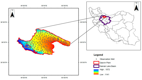
Figure 1.
Study area and location of observation wells (shown with white small circles).
Severe water scarcity is observed in the study area due to rapid growth of water consumption in the agricultural sector, a large number of unauthorized wells, and uncontrolled harvesting. Since surface water resources in the Qazvin Plain area are scarce, groundwater is the main source of water, so the overall extraction has by far exceeded the recharge volume. The groundwater level has fallen by 34 m over the past 50 years [35].
2.2. Pre-Processing Data
One of the main advantages of this study is that all used datasets are openly accessible and free of charge. The coarse-resolution groundwater dataset is obtained from the WGHM-2.2d model version with 0.5 × 0.5-degree resolution. The auxiliary data (i.e., predictors) produced by the ERA5-Land model include evaporation, surface and subsurface runoff, snow depth, and volumetric soil water [36]. Further auxiliary data include the precipitation rate, as provided by the IMERG-GPM satellite-based precipitation product [37]. The time scale of our study spans over 169 months from December 2002 to December 2016. All auxiliary data have a fine spatial resolution of 0.1 × 0.1 degree in the form of absolute values, which were converted into anomalies for the reasons mentioned below.
Time series datasets may contain trends and seasonality, which may need to be removed to be able to use them for further modeling procedures. Trends can result in different means over time, whereas seasonality can result in changing variance over time, both of which define a time series as being non-stationary. Climatological time series data can be disaggregated using harmonic analysis or by seasonal trend decomposition [38] to estimate relative magnitudes of water storage variance in different time series components [39]. We used long-term trends following the aforementioned studies [40,41].
2.2.1. WGHM Hydrologic Model
WGHM is a free access hydrological model developed in 1996 that simulates the continental hydrological variables by including the consequences of domestic, industrial and agricultural consumption on the water resources. This model provides TWS components, i.e., the terrestrial water storage compartments’ snow, soil moisture, groundwater, and surface water bodies, on 67,420 pixels over the globe with a spatial resolution of 0.5 degrees (~50-km) from 1901 onwards. WGHM outputs (e.g., groundwater storage, total water storage, anomalies, and runoff) are the most evaluated against observations [17,21].
2.2.2. ERA5-Land Model
The European Centre for Medium-Range Weather Forecast (ECMWF) ERA5-Land model reanalysis provides variables of the water and energy cycles (e.g., evaporation, surface runoff, subsurface runoff, snow depth, and volumetric soil water). The products are available from January 1981 until three months before the present time in monthly time steps and covers a vertical coverage of 2 m above the surface through soil depth of 289 cm in a total of four layers. Available data, at a resolution of 0.1 × 0.1 degrees (9 × 9 km), will be used as auxiliary variables after conversion into anomalies of, e.g., volumetric soil water.
2.2.3. IMERG-GPM V06b
Goddard Space Flight Center of National Aeronautics and Space Administration (NASA) provides the IMERG-GPM V06b precipitation dataset that includes three-step precipitation rates known as the early, late, and final run. The final run product is available 3.5 months after observation. The data, covering year 2000 and beyond, have a temporal resolution of 30 min and spatial resolution of 0.1° × 0.1° (approximately 10 × 10 km) [42,43]. Based on reported studies over different parts of Iran, the IMERG-GPM product may be the most reliable gridded satellite-based precipitation product [42].
In this study, half-hourly precipitation data were aggregated to a monthly scale and, consequently, converted to anomalies relative to the baseline period from April 2002 to December 2016.
2.2.4. Well Observations
The Qazvin Plain monitoring network was originally put in place in 1964. Now, there are 180 observation wells whose groundwater level data cover the required period of this study (15 years) (Figure 2). In total, 81 wells out of 180 were removed due to significant missing data in the study period. Due to a lack of reliable regional information on specific yield or storativity, the groundwater level (GWL) measurements were not converted to groundwater storage.
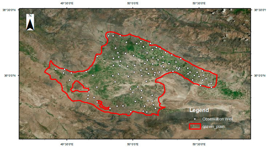
Figure 2.
Location of the selected observation wells.
2.3. Model Development
Different linear regression models, such as the multiple and polynomial linear regression model, K-nearest neighbors and ridge alongside the RF algorithm, are examined to find the most appropriate model. This is carried out during the training-validation step.
Downscaling
The RF model was selected to perform the statistical downscaling of the GWS variable from 0.5° to 0.1°. Presumably, if the predictand and predictors have a meaningful statistical relationship on the origin resolution (0.5° × 0.5°), their relation will be valid on finer resolutions (0.1° × 0.1°). The WGHM-GWS represents the predictand and the water storage components (WSC) as the predictors. Figure 3 illustrates the downscaling procedure.
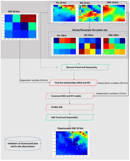
Figure 3.
Schematic view of the workflow of the method.
Before feeding the model with the data, the pre-processing steps should be implemented as follows:
- Preparation Phase
- Spatially resample the auxiliary variables.
- Transform the actual values to anomalies.
- Upscale high spatial resolution auxiliary data (0.1-degree) to the GWS spatial resolution (0.5-degree). Then, Pre, E, SRO, SSRO, snow depth, soil moisture, and STL auxiliary (predictors) monthly time series were shifted from 1 to 10 time steps. The lag was enforced because the variables may have a seasonal relationship with GW changes. The selection of the lag time was based on the correlation coefficient of each variable with GWSA. Predictors were shifted according to their highest correlation values between GWS and the predictors. Generally, the time lag can be identified empirically.
- Remove seasonality and linear trend of all variables to obtain the residuals. This is needed because these parts of data have high variations during this time period and may have a negative effect on the training process of machine learning algorithms [40,41].
- Select a p-value that corresponds to the 0.05 significance level as a criterion to reject the null hypothesis. It should be noted that some high-resolution variables did not show a statistically significant relationship with GWSA, and hence were not involved in the downscaling model.
- Model construction (training phase)
The method adopted in this study assumes that the statistical relationship between the predictor variables and the GWSA at a coarse resolution is maintained at a finer resolution. The statistical relationships between original coarse GWSA and predictors were extracted via models. Input data were randomly partitioned as follows: 80% for training and 20% for validation.
After testing different models, the model with the lowest mean square error (MSE) and highest coefficient of determination () was identified. The RF model outperformed other models used in this study.
- Prediction Phase
To obtain the final downscaled product, the seasonality and long-term trend was added to the RF’s model output in 0.1 degrees (Equation (1)).
It should be mentioned that all the analysis procedures were performed by utilizing the Python programming language, and the ArcGIS.
3. Results
At the first step, the most appropriate model was selected based on their skill scores during the training and validating phase. The RF model outperformed the other trained models with MSE and values of 638.76 and 0.247, respectively, in comparison with the polynomial model with 2 degrees, which showed the highest MSE (807.78) and (0.049) among the rest of the models. The RF Model outperformed the other models and was used in further downscaling procedures.
The time shifting process was considered and a lag was determined as eight months for SWVL, SRO, and SD, where SSRO and STL did not require any time shift. The E and P required seven months lag.
The Qazvin Plain shapefile was provided by Iran Water Resources Management Company (IWRMC). Before and after downscaling, data were evaluated against in situ groundwater level data over the plain for the time period of 2002–2016. After validation, downscaled was examined in terms of trend and seasonality.
Figure 4, Figure 5, Figure 6 and Figure 7 shows the , and in situ water level observations over the study area. The downscaled product covers the study area by 112 pixels, while the original product covers it only by 8 pixels. Figure 4a,c show the maps for April 2010 and August 2010, respectively. Accordingly, Figure 4b,d demonstrate the corresponding downscaled for the same months. These dates were chosen arbitrarily. As can be observed from the downscaled product, the developed downscaling technique is able to capture the spatial distribution features of the original product with higher details.
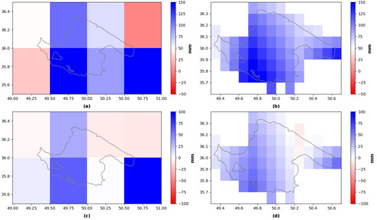
Figure 4.
Spatial distribution of GWSA before and after the downscaling; (a,c) the original 0.5-degree WGHM-GWS data on April 2010 and August 2010; (b,d) the downscaled product at 0.1 degrees in the same month.
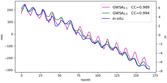
Figure 5.
Comparison of downscaled
and original with in situ groundwater level anomaly (GWLA). The pink, green and blue lines are associated with and (mm), and observations (m).
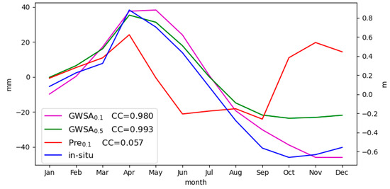
Figure 6.
Plain area average variation in WGHM-based
, downscaled , in situ GW observations, and precipitation anomaly ().
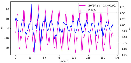
Figure 7.
Plain area average changes in GWSA and in situ observations over Qazvin Plain. Monthly GWLA variation (right y-axis with unit m in EW).
3.1. Groundwater Validation
Since validation of gridded data against point observations is not directly possible, the quality of downscaled was validated at the plain scale. Figure 5 shows the time series of plain area averages of in situ water levels, and . The results also indicated high coefficient correlation values between in situ water livle and GWSA, thus signaling the reliability of WGHM-based GWSA and its downscaled product. It is noteworthy that all products show a decreasing trend for the region.
As already noted, the in situ groundwater level observation has not been converted to groundwater storage. Therefore, Figure 5 has two axes; the left one with the unit of mm corresponds to the GWSA, while the right vertical axis is associated with the in situ GWL anomaly with a unit of m.
A seasonal comparison was also conducted between GWSA products and the observed GWL over the Qazvin Plain (Figure 6). The results show good agreement for seasonal amplitudes between observations with and . The results indicate that the slightly overestimates, while slightly underestimates plain area average observations. Overall, seasonal variations in the in situ GWL anomaly and the and data are highly correlated with 0.98 and 0.99 correlation coefficients, respectively. Generally, the WGHM-based variation follows those of the in situ observation data, while the downscaled effectively simulates the temporal trend of in situ observations.
The lowest groundwater level occurs at the end of the dry season in September, while the highest GW level occurs in April, following periods of precipitation and snowmelt in the absence of irrigation in the region. After April, the GWSA decreases towards the dry months, which might be due to the demand for groundwater withdrawal.
In the same time period, the precipitation anomaly of the plain area average shows that the negative groundwater storage anomaly is greater than the rate anomaly of precipitation, particularly during the warm seasons. However, in the autumn months (Oct–Dec), the precipitation anomaly grows, while the GWSA is much lower in terms of its magnitude, and its slight responses to precipitation can be observed after a few months.
Figure 7 presents the plain area average monthly groundwater changes in downscaled and in situ GWLA over the Qazvin Plain. Good agreement between and the in situ GWLA change is observed in Figure 7, with correlation coefficients of 0.62. Compared with the in situ GWLA changes, GWSA shows good agreement, leading to closer alignment with positive peaks of observations. The results showed a proportional fit but were different in magnitude.
3.2. Trend Analysis
The trend was determined using the Mann–Kendall (MK) test, which, on a yearly basis, was used to determine whether there is a monotonic upward or downward trend in the series.
The trends of the plain area average are shown in Figure 8a,b, respectively, and Figure 9 and Figure 10 illustrate the spatial yearly trend for and . According to Figure 8, overall, the negative trend of GWSA is detected for the scale of the plain area average. However, precipitation trend is −0.35 , and rather negligible in comparison to that of the GWSA trend, which is −34.05 over the Qazvin Plain.
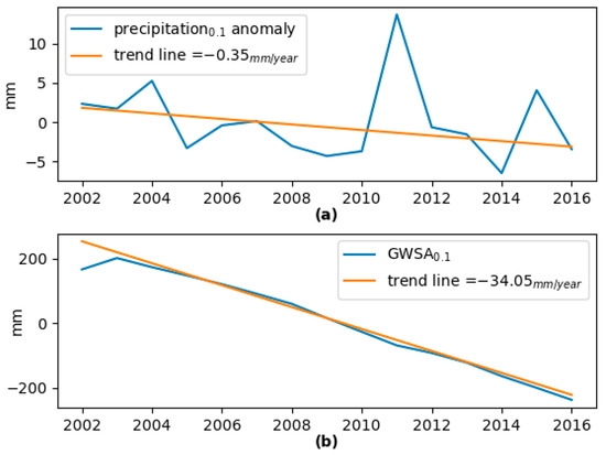
Figure 8.
Qazvin Plain area average (a) and (b) trend on yearly scale.
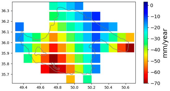
Figure 9.
Qazvin Plain map of long-term GWSA trend in terms of equivalent water thickness (EWT) in mm/year for the WGHM-based (time period is April 2002 to December 2016).
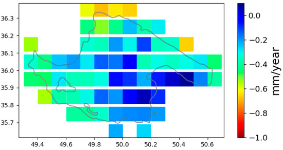
Figure 10.
Qazvin Plain map of long-term precipitation trend in mm/year for anomaly (time period is April 2002 to December 2016).
Figure 9 and Figure 10 show the yearly trend map for both . Figure 9 indicates the decreasing trend of (0~−70 mm annually) in the region during the study time period. follows a slight decreasing trend between 0 and −1 mm annually.
It is noteworthy that follows a sharp declining annual trend. Although the annual precipitation anomaly trend also decreases, the magnitude of the precipitation anomaly is quite small in comparison to that of groundwater storage changes (GWSC). In other words, one can say that the decreasing precipitation anomaly minimally contributes to the decreasing GWSA. This result is also consistent with other studies in this region that showed groundwater depletion, resulting from human withdrawals for agriculture, is a major cause for the sharp declining groundwater table [9,35].
4. Conclusions
The main purpose of this study is to downscale the GWSA of the WGHM from a coarse (0.5 degree) to a finer spatial resolution (0.1 degree) by using fine spatial resolution auxiliary datasets (0.1-degree), such as evaporation, surface and subsurface runoff, snow depth, and volumetric soil water, from the ERA5-Land model, as well as the IMERG product. However, other satellite-based products, such as land use and drought indices, might be helpful predictors.
In this study, predictors (auxiliary datasets) and regression models are used for downscaling gridded GW storage. Moreover, different linear regression models, such as the multiple and polynomial linear regression model, K-nearest neighbors, ridge, and RF techniques, were examined to find the most appropriate model. The RF model showed that its performance is far superior to MLR and the polynomial approach. The RF model also outperformed other models and was adopted for the downscaling procedure.
This study improved the spatial resolution of the monthly WGHM-based groundwater storage anomaly (GWSA) from 0.5 degrees to 0.1 degrees. The downscaling procedure supports various water-related studies that involve the fine spatial resolution of GWSA products as input to water resource planning reports, as well as to regional hydrological modeling efforts.
The performance of downscaled was satisfactorily compared with its original and in situ GW table level variation from 2002 to 2016 over the Qazvin Plain, Iran. The plain area average comparison between the in situ well observations confirmed that the downscaled products maintained the accuracy of the original . The results showed a superb correlation coefficient of 0.994 and 0.989 between GWLA and and , respectively, which imply the reliability of WGHM-based GWSA and its downscaled product. The seasonal validation shows good agreement between observations with and with correlation coefficients of 0.99 and 0.98, respectively.
Moreover, the trend analysis showed a sharp declining annual trend for . Although the annual precipitation trend is declining, the contribution of precipitation is quite small in comparison to that of GWSA. The effect of water abstractions and reservoir management on GWSA trends can be evaluated qualitatively by comparing GWSA trends with irrigation intensities, although previous studies highlighted that the large GWSA declines in this region are due to heavy irrigation.
However, the GWSA can be calibrated with in situ observations to improve the accuracy, but this needs to be reliable and well distributed within an aquifer or on a global scale, which is challenging. Moreover, using different artificial intelligence techniques can create an opportunity to predict the missing values during the study period. These models can reduce the possible smoothness that may occur during the (NaN) value filtrations. It can also estimate more robust results for the upcoming months [44]. The developed RF model can predict further GWSA after 2016 until the available date of the predictors’ products. By predicting/forecasting the upcoming months for GWL regimes, evaluation of the results would be improved and it provides a better perspective for governing plans.
The main concentration of this study has been improving the spatial distribution information. For evaluating the accuracy of the predicted values, it is necessary to convert the GWL to GWS. This conversion requires precise hydrogeological information on the study region, and study cases that have a lack of sufficient in situ details are encouraged to pursue their evaluations using the GWL [7,40,41].
Moreover, temporal downscaling of GWSA from monthly to weekly or daily is challenging, since the relationships between environmental variables and GWSA on these scales are far less evident and difficult to capture; however, it needs further assessment. Furthermore, the proposed downscaling methodology may lead to future updates of GW maps derived from ongoing models and satellite missions. For example, the Global Gravity-based Groundwater Product (G3P) is currently developing a product to extract the GWSA on satellite observations on a global scale.
The results showed that the proposed downscaling method is able to learn from the fine spatial resolution of auxiliary data (predictors) and resolve the spatial features of GWSA over the plain. In general, the downscaling method used in this study is robust, accurate, and easy to use, showing promising results in the study area. Thus, it may be adopted and tested in other regions, where groundwater data of higher spatial resolution are needed. In addition, the main advantage of the proposed methodology lies in the use of auxiliary (input) data that are freely available with global coverage, making it possible to apply the method to other geographical regions. Another advantage is that in this method, the GW data are needed only for the time duration of the training phase. It means that in case there are no GW data with coarse spatial resolution (e.g., 0.5 degree) available, the model can predict/estimate the GW at a finer scale (0.1 degree), by using only the auxiliary data. It is recommended to study artificial intelligence techniques with various architectures and optimization, and input combinations in future works.
Author Contributions
Conceptualization, B.S. and E.S.; methodology, E.S.; software, S.Z.D., R.R. and E.S.; validation, S.Z.D., R.R. and E.S.; data curation, E.S.; writing—original draft preparation, S.Z.D. and E.S.; writing—review and editing, S.Z.D., E.S. and B.S.; supervision, E.S. and B.S. All authors have read and agreed to the published version of the manuscript.
Funding
This study has received funding from the European Union’s Horizon 2020 research and innovation programme for G3P (Global Gravity-based Groundwater Product) under grant agreement n° 870353.
Conflicts of Interest
The authors declare no conflict of interest.
References
- Güntner, A. Towards an Operational Copernicus Service: A Global Gravity-based Groundwater Product (G3P). In AGU Fall Meeting Abstracts; American Geophysical Union: Washington, DC, USA, 2020; Volume 2020, p. H079-06. [Google Scholar]
- Bojinski, S.; Verstraete, M.; Peterson, T.C.; Richter, C.; Simmons, A.; Zemp, M. The concept of essential climate variables in support of climate research, applications, and policy. Bull. Am. Meteorol. Soc. 2014, 95, 1431–1443. [Google Scholar] [CrossRef]
- Famiglietti, J.S. The global groundwater crisis. Nat. Clim. Chang. 2014, 4, 945–948. [Google Scholar] [CrossRef]
- Döll, P.; Fiedler, K. Global-scale modeling of groundwater recharge. Hydrol. Earth Syst. Sci. 2008, 12, 863–885. [Google Scholar] [CrossRef]
- Turkeltaub, T.; Bel, G. The effects of rain and evapotranspiration statistics on groundwater recharge estimations under semi-arid environments. Hydrol. Earth Syst. Sci. Discuss. 2022, 1–23. [Google Scholar] [CrossRef]
- Herrera-Pantoja, M.; Hiscock, K.M. The effects of climate change on potential groundwater recharge in Great Britain. Hydrol. Process. 2008, 22, 73–86. [Google Scholar] [CrossRef]
- Sahoo, S.; Chakraborty, S.; Pham, Q.B.; Sharifi, E.; Sammen, S.S.; Vojtek, M.; Vojteková, J.; Elkhrachy, I.; Costache, R.; Linh, N.T.T. Recognition of district-wise groundwater stress zones using the GLDAS-2 catchment land surface model during lean season in the Indian state of West Bengal. Acta Geophys. 2021, 69, 175–198. [Google Scholar] [CrossRef]
- doostan, reza Analysis of Drought Researches of Iran. J. Spat. Anal. Environ. Hazarts 2020, 6, 53–94. [CrossRef]
- Samani, S. Analyzing the Groundwater Resources Sustainability Management plan in Iran through Comparative Studies. Groundw. Sustain. Dev. 2021, 12, 100521. [Google Scholar] [CrossRef]
- Saemian, P.; Tourian, M.J.; AghaKouchak, A.; Madani, K.; Sneeuw, N. How much water did Iran lose over the last two decades? J. Hydrol. Reg. Stud. 2022, 41, 101095. [Google Scholar] [CrossRef]
- Taghizadeh, E.; Ahmadi-Givi, F.; Brocca, L.; Sharifi, E. Evaluation of satellite/reanalysis precipitation products over Iran. Int. J. Remote Sens. 2021, 42, 3474–3497. [Google Scholar] [CrossRef]
- Döll, P.; Kaspar, F.; Lehner, B. A global hydrological model for deriving water availability indicators: Model tuning and validation. J. Hydrol. 2003, 270, 105–134. [Google Scholar] [CrossRef]
- Werth, S.; Güntner, A.; Petrovic, S.; Schmidt, R. Integration of GRACE mass variations into a global hydrological model. Earth Planet. Sci. Lett. 2009, 277, 166–173. [Google Scholar] [CrossRef]
- Werth, S.; Güntner, A. Calibration analysis for water storage variability of the global hydrological model WGHM. Hydrol. Earth Syst. Sci. 2010, 14, 59–78. [Google Scholar] [CrossRef]
- Schumacher, M.; Forootan, E.; van Dijk, A.I.J.M.; Müller Schmied, H.; Crosbie, R.S.; Kusche, J.; Döll, P. Improving drought simulations within the Murray-Darling Basin by combined calibration/assimilation of GRACE data into the WaterGAP Global Hydrology Model. Remote Sens. Environ. 2018, 204, 212–228. [Google Scholar] [CrossRef]
- Rodell, M.; Houser, P.R.; Jambor, U.; Gottschalck, J.; Mitchell, K.; Meng, C.J.; Arsenault, K.; Cosgrove, B.; Radakovich, J.; Bosilovich, M.; et al. The Global Land Data Assimilation System. Bull. Am. Meteorol. Soc. 2004, 85, 381–394. [Google Scholar] [CrossRef]
- Müller Schmied, H.; Caceres, D.; Eisner, S.; Flörke, M.; Herbert, C.; Niemann, C.; Asali Peiris, T.; Popat, E.; Theodor Portmann, F.; Reinecke, R.; et al. The global water resources and use model WaterGAP v2.2d: Model description and evaluation. Geosci. Model Dev. 2021, 14, 1037–1079. [Google Scholar] [CrossRef]
- van der Knijff, J.M.; Younis, J.; de Roo, A.P.J. LISFLOOD: A GIS-based distributed model for river basin scale water balance and flood simulation. Int. J. Geogr. Inf. Sci. 2010, 24, 189–212. [Google Scholar] [CrossRef]
- Sutanudjaja, E.H.; Van Beek, R.; Wanders, N.; Wada, Y.; Bosmans, J.H.C.; Drost, N.; Van Der Ent, R.J.; De Graaf, I.E.M.; Hoch, J.M.; De Jong, K. PCR-GLOBWB 2: A 5 arcmin global hydrological and water resources model. Geosci. Model Dev. 2018, 11, 2429–2453. [Google Scholar] [CrossRef]
- Fang, H.; Beaudoing, H.K.; Teng, W.L.; Vollmer, B.E. Global Land data assimilation system (GLDAS) products, services and application from NASA hydrology data and information services center (HDISC). In Proceedings of the ASPRS 2009 Annual Conference, Baltimore, MD, USA, 9–13 March 2009. [Google Scholar]
- Alcamo, J.; Döll, P.; Henrichs, T.; Kaspar, F.; Lehner, B.; Rösch, T.; Siebert, S. Development and testing of the WaterGAP 2 global model of water use and availability. Hydrol. Sci. J. 2003, 48, 317–337. [Google Scholar] [CrossRef]
- Yin, W.; Zhang, G.; Liu, F.; Zhang, D.; Zhang, X.; Chen, S. Improving the spatial resolution of GRACE-based groundwater storage estimates using a machine learning algorithm and hydrological model. Hydrogeol. J. 2022, 30, 947–963. [Google Scholar] [CrossRef]
- Yin, W.; Hu, L.; Zhang, M.; Wang, J.; Han, S.C. Statistical Downscaling of GRACE-Derived Groundwater Storage Using ET Data in the North China Plain. J. Geophys. Res. Atmos. 2018, 123, 5973–5987. [Google Scholar] [CrossRef]
- Fowler, H.J.; Blenkinsop, S.; Tebaldi, C. Linking climate change modelling to impacts studies: Recent advances in downscaling techniques for hydrological modelling. Int. J. Climatol. 2007, 27, 1547–1578. [Google Scholar] [CrossRef]
- Tang, J.; Niu, X.; Wang, S.; Gao, H.; Wang, X.; Wu, J. Statistical downscaling and dynamical downscaling of regional climate in China: Present climate evaluations and future climate projections. J. Geophys. Res. 2016, 121, 2110–2129. [Google Scholar] [CrossRef]
- Wang, Z.; Lai, C.; Chen, X.; Yang, B.; Zhao, S.; Bai, X. Flood hazard risk assessment model based on random forest. J. Hydrol. 2015, 527, 1130–1141. [Google Scholar] [CrossRef]
- Shi, Y.; Song, L. Spatial downscaling of monthly TRMM precipitation based on EVI and other geospatial variables over the Tibetan Plateau from 2001 to 2012. Mt. Res. Dev. 2015, 35, 180–194. [Google Scholar] [CrossRef]
- Chaney, N.W.; Wood, E.F.; McBratney, A.B.; Hempel, J.W.; Nauman, T.W.; Brungard, C.W.; Odgers, N.P. POLARIS: A 30-meter probabilistic soil series map of the contiguous United States. Geoderma 2016, 274, 54–67. [Google Scholar] [CrossRef]
- Pang, B.; Yue, J.; Zhao, G.; Xu, Z. Statistical downscaling of temperature with the random forest model. Adv. Meteorol. 2017, 2017, 7265178. [Google Scholar] [CrossRef]
- Breiman, L. Bagging predictors. Mach. Learn. 1996, 24, 123–140. [Google Scholar] [CrossRef]
- Rahimi Rahbar, S.R. Downscaling of Groundwater Images Using Machine Learning Techniques, The University of Applied Sciences Campus Vienna. 2022. Available online: https://pub.fh-campuswien.ac.at/obvfcwhs/content/titleinfo/7884456 (accessed on 7 September 2022).
- Barahimi, M.; Shahverdi, K. Updating and Reviewing of the Document of National Water in Ghazvin and Fomanat Plains. J. Water Soil Sci. 2018, 22, 199–209. [Google Scholar] [CrossRef]
- Abkhan Consulting Engineers. Water Resources Balance Report Studies of Qazvin: The Study Areas of the Salt Lake Watershed; Abkhan Consulting Engineers: Tehran, Iran, 2013; Available online: https://www.abkhan-co.com/en.html (accessed on 19 June 2021).
- Babaee, S.; Mousavi, Z.; Masoumi, Z.; Malekshah, A.H.; Roostaei, M.; Aflaki, M. Land subsidence from interferometric SAR and groundwater patterns in the Qazvin plain, Iran. Int. J. Remote Sens. 2020, 41, 4780–4798. [Google Scholar] [CrossRef]
- Sanginabadi, H. Groundwater Regional Risk Analysis during Droughts and Determination of Warning Thresholds, 2019. Ph.D. Thesis, Islamic Azad University, Science and Research Branch, Tehran, Iran, 2019. [Google Scholar]
- Muñoz-Sabater, J. ERA5-Land hourly data from 1950 to 1980. Copernicus Clim. Chang. Serv. Clim. Data Store 2021. [Google Scholar] [CrossRef]
- Tan, J.; Huffman, G.J.; Bolvin, D.T.; Nelkin, E.J.; Rajagopal, M. SHARPEN: A scheme to restore the distribution of averaged precipitation fields. J. Hydrometeorol. 2021, 22, 2105–2116. [Google Scholar] [CrossRef]
- Humphrey, V.; Gudmundsson, L.; Seneviratne, S.I. Assessing global water storage variability from GRACE: Trends, seasonal cycle, subseasonal anomalies and extremes. Surv. Geophys. 2016, 37, 357–395. [Google Scholar] [CrossRef]
- Scanlon, B.R.; Zhang, Z.; Rateb, A.; Sun, A.; Wiese, D.; Save, H.; Beaudoing, H.; Lo, M.H.; Müller-Schmied, H.; Döll, P. Tracking seasonal fluctuations in land water storage using global models and GRACE satellites. Geophys. Res. Lett. 2019, 46, 5254–5264. [Google Scholar] [CrossRef]
- Tangdamrongsub, N.; Jasinski, M.F.; Shellito, P.J. Development and evaluation of 0.05° terrestrial water storage estimates using Community Atmosphere Biosphere Land Exchange (CABLE) land surface model and assimilation of GRACE data. Hydrol. Earth Syst. Sci. 2021, 25, 4185–4208. [Google Scholar] [CrossRef]
- Vishwakarma, B.D.; Zhang, J.; Sneeuw, N. Downscaling GRACE total water storage change using partial least squares regression. Sci. Data 2021, 8, 95. [Google Scholar] [CrossRef] [PubMed]
- Sharifi, E.; Steinacker, R.; Saghafian, B. Assessment of GPM-IMERG and other precipitation products against gauge data under different topographic and climatic conditions in Iran: Preliminary results. Remote Sens. 2016, 8, 135. [Google Scholar] [CrossRef]
- Huffman, G.; Bolvin, D.; Braithwaite, D.; Hsu, K.; Joyce, R.; Xie, P.; Yoo, S. Algorithm Theoretical Basis Document (ATBD) Version 06. NASA Global Precipitation Measurement (GPM) Integrated Multi-Satellite Retrievals for GPM (IMERG), NASA. 2019. Available online: https//pmm.nasa.gov/data-access/downloads/gpm (accessed on 4 December 2019).
- Vadiati, M.; Rajabi Yami, Z.; Eskandari, E.; Nakhaei, M.; Kisi, O. Application of artificial intelligence models for prediction of groundwater level fluctuations: Case study (Tehran-Karaj alluvial aquifer). Environ. Monit. Assess. 2022, 194, 619. [Google Scholar] [CrossRef]
Publisher’s Note: MDPI stays neutral with regard to jurisdictional claims in published maps and institutional affiliations. |
© 2022 by the authors. Licensee MDPI, Basel, Switzerland. This article is an open access article distributed under the terms and conditions of the Creative Commons Attribution (CC BY) license (https://creativecommons.org/licenses/by/4.0/).