Abstract
Accurate streamflow prediction is significant when developing water resource management and planning, forecasting floods, and mitigating flood damage. This research developed a novel methodology that involves data pre-processing and an artificial neural network (ANN) optimised with the coefficient-based particle swarm optimisation and chaotic gravitational search algorithm (CPSOCGSA-ANN) to forecast the monthly water streamflow. The monthly streamflow data of the Tigris River at Amarah City, Iraq, from 2010 to 2020, were used to build and evaluate the suggested methodology. The performance of CPSOCGSA was compared with the slim mold algorithm (SMA) and marine predator algorithm (MPA). The principal findings of this research are that data pre-processing effectively improves the data quality and determines the optimum predictor scenario. The hybrid CPSOCGSA-ANN outperformed both the SMA-ANN and MPA-ANN algorithms. The suggested methodology offered accurate results with a coefficient of determination of 0.91, and 100% of the data were scattered between the agreement limits of the Bland–Altman diagram. The research results represent a further step toward developing hybrid models in hydrology applications.
1. Introduction
Water shortages have become a global concern due to the rapid increase in residential, industrial, and agricultural demand, as well as the growing need to conserve water in order to maintain ecosystem services [1]. Socio-economic factors (i.e., urbanization, population growth, and industry) and climate change are intensifying water scarcity—where water needs exceed availability—for cities worldwide [2]. The United Nations estimates that about 1.8 billion people will face water scarcity by 2025, and two-thirds of the world’s population will be water stressed [3]. Different basins globally face predominant water stress and associated water resource quantity and quality challenges that adversely impact sustainable development, especially for developing countries [4].
Iraq is one developing country that suffers from the vulnerability of climate change (i.e., increased temperature and reduced rainfall). Additionally, socio-economic factors (i.e., urbanization, population growth, and the oil industry) impact freshwater resources. The Tigris and Euphrates Rivers are the principal water resources in Iraq that experienced significant water shortages from 2009 to 2014. Water scarcity is predicted to increase due to climate change, increasing water consumption upstream (Turkey, Iran, and Syria) [5]. There is also evidence that the temperature in Iraq will rise two to seven times faster than the world average, according to Salman et al. [6]. Furthermore, Iraq’s future rainfall patterns and amounts are anticipated to be significantly affected based on various forms of analyses and scenarios [7].
Therefore, forecasting is considered essential for water conservation and ensuring environmental sustainability, as has been proven in various fields [8,9]. Forecasting streamflow over time is critical for a variety of reasons, including water supply reliability, drought and flood risk, and environmental maintenance security. Long-term accurate streamflow forecasts help with water resource planning and management [10]. On the other hand, river flow modelling is a complex undertaking, as river flow time series are frequently random, dynamic, non-linear, and chaotic [11]. An analysis of the univariate streamflow predictions by Zhang et al. [12] found that data-driven models are widely used because of their simplicity and minimal data needs. The most frequently artificial intelligence (AI) models used in streamflow forecasting are neural-based fuzzy inference systems (ANFIS) [13], support vector machines (SVM) [14], and artificial neural networks (ANN) [15]. As a simple operational model, ANN offers significant non-linear mapping capabilities [10]. Despite the many successes that have resulted from employing the ANN method with a single ANN, there is still a lot of space for development [16]. This has encouraged researchers to improve their models. However, various hybrid models incorporating ANNs and various optimization strategies have been created [17].
Therefore, instead of applying a single model to the same data, a hybrid technique combines the benefits of two or more independent models to increase prediction accuracy [18], as in streamflow forecasting [19,20,21]. Additionally, it has been discovered that the accuracy of AIs (without pre-processing data methods) can be enhanced by combining hybrid AI models (which contain coupled models) with data pre-processing processes [22]. In addition, the findings of some studies have demonstrated that hybrid models are both robust and informative, and they have been successfully used in various hydrological fields, for example in water demand forecasting [23,24] and rainfall forecasting [25].
In the same context, the literature has emphasized the importance of applying data pre-processing to enhance time series quality and identify the best predictor scenarios. The importance of data cleaning has grown in recent years. Consequently, several signal pre-treatment strategies have been used to eliminate noise in streamflow time series, such as wavelet transform (WT) [26], singular spectrum analysis (SSA) [27], empirical mode decomposition (EMD) [28], and variational mode decomposition (VMD) [29]. Another substantial aspect of data pre-processing is choosing the best scenario for predictors, such as mutual information (MI) [30], for a univariate model. Using non-linear statistical dependence metrics, such as MI, is more suitable for selecting inputs for ANN techniques than a correlation, which has the limitation of only assessing the linear relationship between variables [31].
Recently, Ibrahim et al. [32] reviewed the streamflow simulating models and stated that machine learning (ML) techniques also need to be optimized in tandem to perform the optimum outcome, thus leading to the desirous formation of combined methods between a single ML model and optimization techniques. Additionally, the study recommended that (1) the pre-processing data stage is advisable to be done as efficiently as possible to avoid noise in the data. In addition, it is suggested that more focus should be allocated to determining the best predictor combination. (2) Model hyperparameters (i.e., the learning rate coefficient in ANN) are one of the most important aspects influencing the model’s performance and results. So, selecting and tuning those hyperparameters is recommended by applying metaheuristic algorithms instead of utilizing a trial and error procedure.
The search for the best possible solution within a large and uncertain space is a classic optimization problem that arises in many different branches of engineering. Numerical methods may be useful when an analytical solution is impossible or would take too long to implement in practice, but they cannot guarantee a globally optimal result because there is a high possibility of falling in the local minima. There are a variety of metaheuristic algorithms that obtain their motivation primarily from nature. Hybridization of existing algorithms is another prevalent strategy for improving algorithm performance, alongside developing new metaheuristic algorithms [33]. In addition, the No Free Lunch Theorem (NFLT) [34] mentions that no single algorithm can effectively address all possible optimization scenarios. In other words, even if an optimization technique achieves an excellent performance for some issues, it likely performs poorly for others. This has led to the development of a wide variety of methods for solving optimization problems that have been proposed by the scientific community.
Several metaheuristic-based methodologies have been developed to determine the optimal tuning of forecasting models [35]. In recent years, various metaheuristic algorithms have been effectively utilized in the subject of hydrology. Li et al. [36] created the slim mold algorithm (SMA), which is a contemporary nature-inspired algorithm that has been used to solve a variety of optimization problems, such as those in photovoltaic solar systems [37]. Additionally, the marine predator algorithm (MPA) is a population-based meta-heuristic algorithm [38] that has been used to tackle various optimization issues, such as power resources [39]. Furthermore, the particle swarm optimization (PSO) algorithm was originally designed to model social behavior because of its ability to optimize complex numerical functions [8]. The PSO method generally provides better problem-solving abilities, a high convergence speed, and good generalization capabilities for a wide range of situations [9].
The two primary features of metaheuristic algorithms are exploration and exploitation. In computer science, “exploration” refers to the bounds of the algorithm’s search space, whereas “exploitation” is the practice of selecting the most optimal answer from among several possible ones [40]. The exploration and exploitation are inversely proportional to each other, as stated by Eiben and Schippers [41]. This means that if an optimization method has excellent exploration power for one problem, it will have low exploitation power for another. The optimization algorithms are hybridized to overcome the randomization, intensification, and entrapment in local minima issues. Furthermore, hybridization improves the algorithms’ efficiency and accuracy [40]. Accordingly, Rather and Bala [40] developed the constriction coefficient-based particle swarm optimization and chaotic gravitational search algorithm (CPSOCGSA). To achieve the best outcome, it integrates PSO’s exploitative abilities with those of GSA’s exploratory ones. In addition, it employs 10 chaotic maps for optimal balance between exploration and exploitation processes.
Recently, Hajirahimi and Khashei [42] reviewed the hybridization of hybrid structures for time series predicting, and the study demonstrated that pre-processing data and optimization algorithms are crucial components of hybridization. The hybridization of hybrid models, wherein two or more hybrid classes are merged as opposed to combining the typical individual forecasting methods, is a novel idea suggested in recent literature in order to reach a high accuracy. One of these techniques that was applied successfully is the hybridization of preprocessing-based with parameter optimization-based hybrid models (HPOH). The hybridization of hybrid models also has certain research gaps that need to be addressed and future research directions that need to be explored. Moreover, Magali Troin and Martel [43] reviewed the techniques and methods of streamflow prediction over 40 years and stated that hybrid prediction models are currently a well-established topic of study that covers a wide range of operational scenarios. In addition, Ibrahim et al., 2022 [32], concluded that ML techniques have an opportunity for growth and consideration for future hybrid AI modelling that will make the hydrological study even more intriguing, demanding, and rewarding for academics. This study aims to develop a novel methodology that can accurately forecast monthly medium-term streamflow considering previous streamflow data. In order to do this, the following tasks will be achieved:
- (1)
- Applying the pre-processing data stage to enhance the data quality through the singular spectrum analysis (SSA) method and to select the best predictor (lags) scenario using the mutual information (MI) technique.
- (2)
- Integrating the ANN model with the coefficient-based particle swarm optimization and chaotic gravitational search algorithm (CPSOCGSA-ANN) to forecast the monthly water streamflow.
- (3)
- Examining the performance of the CPSOCGSA-ANN algorithm by applying a hybrid slim mold algorithm (SMA-ANN) and marine predator algorithm (MPA-ANN).
- (4)
- Applying the HPOH technique for simulating the monthly streamflow based on several lags.
- (5)
- Expanding the forecasting range and decreasing the uncertainty level of outcomes for monthly streamflow simulation by testing different recent metaheuristic algorithms (i.e., hybridization of two existing and two recent algorithms).
2. Study Area and Data Used
The main sources of freshwater in Iraq are the Euphrates and Tigris Rivers. The Tigris River is one of the main rivers in the Middle East. The river is 1718 km long altogether and flows through Turkey, Syria, and Iraq, with about 85% of the total basin of the Tigris River lying in Iraq [44].
Amarah is the capital of the Maysan Governorate in southern Iraq (Figure 1). The study area is defined by longitudes (46°20′–48°05′ E) and latitudes (31°10′–32°50′ N), located 400 km south-east of Baghdad Province. Additionally, the area of Maysan Governorate covers around 16,683 km2 [45]. Amara has a characteristic climate with hot summers and chilly winters. In the summer, high temperatures are frequently over 40 °C. Precipitation falls during winter and averages 177 mm annually [46].
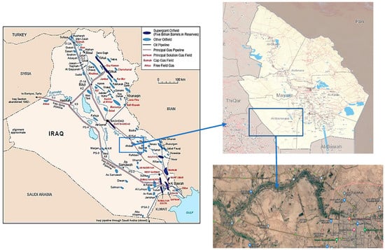
Figure 1.
Study area, Amarah City, Iraq.
Historical monthly streamflow (m3/s) data were gathered from 2010–2020, supplied by the Directorate of Water Resources in Maysan City, and were used to build and assess the model. Figure 2 presents the time series and box plot of the monthly Tigris River streamflow at Amarah City.
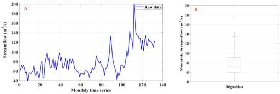
Figure 2.
(A) Monthly streamflow time series; (B) box plot for the Tigris River streamflow at Amarah City.
3. Methodology
The suggested methodology can be separated into four aspects: data pre-processing, artificial neural networks, the CPSOCGSA algorithm, and model validation, as shown in Figure 3.
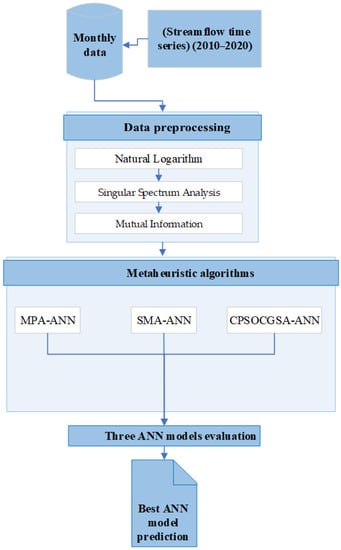
Figure 3.
A scheme of the proposed methodology to simulate the monthly streamflow data.
3.1. Data Pre-Processing
Recent improvements in streamflow forecasting methodologies underline the need to use various data pre-processing approaches, which can be divided into three categories: normalization, cleaning, and selecting the optimal model input [23]. Following Zubaidi et al. [47], using the SPSS 24 statistics tool, the natural logarithm was applied to normalize the time series and to eliminate multi-collinearity between independent variables (model input).
The data cleaning method involves detecting and treating unwanted or worthless data in order to improve the prediction results. The outliers’ data have a negative impact on the regression solution and the model’s accuracy [23]. After normalization, the outliers’ data were determined using the box and whisker method, and then the scores were adjusted to fit the remainder of the data. Then, normalized and clean time series data were denoised using singular spectrum analysis (SSA).
SSA is a relatively effective approach for decomposing the original time series into multiple principal components (PCs). Every PC explains a proportion of the variance of the original time series, where the first component has the largest value and the last component has the lowest proportion. SSA can be used for the purpose of time series denoising by selecting the PCs with the largest proportions of variance and neglecting the PCs with the smallest variance proportions, which usually explains the structureless noise in the time series [48]. This approach has proven to be successful in a variety of fields, such as streamflow forecasting [27], drought forecasting [49], and industry [50]. More information on SSA can be found in Zhigljavsky [51].
Selecting a suitable predictor’s scenario is one of the most crucial steps for developing the structure of the prediction model. This phase improves the model’s performance by identifying the most significant factors [47]. In order to choose the most effective explanatory variables, the mutual information (MI) technique was applied in this study. Danandeh Mehr et al. [52] stated that the average mutual information (AMI) is a non-linear generalization of the autocorrelation function. Mutual information is commonly utilized to locate time-delayed independent variables.
3.2. Artificial Neural Network (ANN)
Artificial neural networks (ANNs) use a model structure similar to a human brain’s neural network. ANN is an effective computational method for representing non-linear systems [53]. The capacity of the ANN model to uncover complicated non-linear relationships has led to its popularity in water resources and hydrological areas, as in S.I.Abbaa et al. [54], Tiu et al. [55], and Zubaidi et al. [23]. The most popular ANN design is the multi-layer feedforward neural network (MLFFNN), because it is easy to implement. Their primary benefit is that they can provide a simulation for any input/output map, while also being quite straightforward to implement. When it comes to containing a neural network’s error rate, the Levenberg Marquardt (LM) algorithm is frequently employed because it is a high-demand, flexible calculation [56]. There are three primary layers in an MLP model: the input layer, the hidden layer, and the output layer. Thomas et al. [57] investigated whether MLFFNN with two hidden layers improves generalization over those with one. The study concluded that networks with two hidden layers were superior at generalizing nine out of ten cases, although the actual degree of enhancement was case-dependent. In addition, multiple studies have demonstrated the efficacy of ANNs with two hidden layers in capturing the nonlinear relationship between the simulated and observed [47,58,59]. To have the same ANN structure as in Zubaidi et al. [47], this research will use the ANN model with four layers, including the input (received Lags of streamflow), two hidden layers, and an output layer (target, future streamflow). The trial and error procedure establishes the ideal learning rate and the number of neurons for the hidden layers. However, this approach is inefficient and may not yield the best results [47]. Therefore, the CPSOGSA-ANN, MPA-ANN, and SMA-ANN algorithms were used to determine the learning rate coefficient, the number of neurons in both hidden layers, and to prevent over- or under-fitting the model. In addition, the hybrid techniques enhanced the ANN model’s performance and saved time.
The entire data set was divided into three portions: training (70%), testing (15%), and validation (15%) [27]. Each ANN model was run multiple times to determine the optimal neural network structure (weights) for effectively predicting the streamflow.
3.3. Hybridized Constriction Coefficient-Based Particle Swarm Optimization and Chaotic Gravitational Search Algorithm (CCPSOCGSA)
It is widely documented that each algorithm has inherent limitations that reduce its ability to produce reliable and sound estimates. As such, the concept of merging two different algorithms has been increasingly used to cope with the aforementioned issue. Accordingly, the hybridized constriction coefficient-based particle swarm optimization and chaotic gravitational search algorithm (CCPSOCGSA) was developed by combining the particle swarm optimization (PSO) technique, which reflects the simulated behavior of bird flocking, and the gravitational search algorithm (GSA), in which Newton’s law of universal gravitation is the driving principle of this physics-based heuristic technique. The CCPSOCGSA technique has the advantages of the merits of PSO and GSA and diminishes the drawbacks associated with PSO and GSA techniques represented by randomization, intensification, and local minima. The detailed information regarding this hybridized technique will be elaborated on in the next subsections.
3.3.1. Constriction Coefficient-Based Particle Swarm Optimization (CCPSO)
The electrical engineer Russell C. Eberhart and the social psychologist James Kennedy first developed the PSO technique. They were inspired by the behavior of fish or a flock of birds in their search for food to propose this algorithm. This behavior shows that a group of fish and/or a flock of birds can profit from the experience of all other group members to hunt best, reduce the time of that journey, and save energy. In terms of complexity, PSO is deemed to be the simplest algorithm compared with the others. Three main operators, namely, inertia weight, pbest, and gbest constitute the main structure of the PSO algorithm. The first operator plays a significant role in the global exploration process, while the rest of the operators help find the search space region. The updating process of the location and velocity of the particles during the change of their values (particle values) can be mathematically described as below:
where c1 and c2 are the learning constants, while are numbers ranging from 0 to 1.
It should be noted that the CCPSO algorithm was developed to overcome the drawbacks and limitations associated with PSO. These issues can limit the ability of PSO to compete with other algorithms in terms of estimation accuracy. To be specific, PSO has inherent limitations, namely, particle movements outside the solution space and the time of convergence during the optimization process [60]. The constriction coefficient is as described below:
where K represents the constriction coefficient, which embodies the inertia weight. Equation (1) can be rewritten as follows:
where ,
3.3.2. Chaotic Gravitational Search Algorithm CGSA
The GSA algorithm was developed by taking advantage of a physical phenomenon, namely, Newton’s law of gravitation and motion. This law helps attract agents (objects) through gravitational force, which plays a key role in this regard. Objects with heavier masses pull other objects with lower masses. It is noteworthy that each mass has four specifications: position, inertial mass, active gravitational mass, and passive gravitational mass. The solution to the problem of GSA is usually associated with the position of the mass, while the gravitational and inertial masses are determined using a fitness function. The mathematical formulation of the gravitational force between masses x and y at time t can be written as in Equation (6):
where denote passive and attractive masses, respectively. Rxy (t) is the Euclidian distance between the two masses at time t, while is a small value to avoid division by zero [61]. The constant G helps in controlling the solution space and finding the feasible region, and can be represented by Equation (7):
where are the final and initial values of G, respectively, is a small constant, is the current iteration, and is the maximum number of iterations.
The change in G over time is described using a chaotic normalization process [40,62], and the final representation of the gravitational constant can be formulated by Equation (8):
The total force exerted by the masses can be described in Equation (9) below:
where is a constant with a range between 0 and 1.
To help find the global optimum, the position and velocity of the heavy search agent (i.e., mass) should be calculated. The position and velocity can be written as in Equations (10) and (11):
where is the acceleration of the mass.
3.3.3. Combination of CCPSO and CGSA
The aforementioned two techniques (CPSO and CGSA) can be merged to obtain an advantage from the strengths of each approach and to overcome their limitations. By doing so, the analyst can obtain solid and reliable estimates. The hybridization equation formula can be described as in Equation (12):
The location of the particles is given by Equation (13):
3.4. Model Validation
The effectiveness of the proposed methodology was assessed using the mean absolute error (MAE), root mean squared error (RMSE), mean absolute relative error (MARE), scatter index (SI), mean bias error (MBE), and the coefficient of determination These indicators are defined in Equations (14)–(19). Additionally, graphical plots, such as a Taylor diagram, Bland–Altman, and scatter plot, were utilized to evaluate the forecasting effectiveness of the proposed methodology.
where Oi is the measured streamflow, Fi is the predicted streamflow, is the mean of the measured streamflow, is the mean of the predicted streamflow, and N is the length of the data.
4. Results and Discussion
4.1. Preparation of the Target and Predictors Factors
Firstly, data were normalized by applying the natural logarithm and were cleaned. Then, the SSA method was used to gain the time series data of the streamflow without noise (this was achieved by analyzing the normalized and cleaned time series into three components); these steps are according to Section 3.1. Figure 4 displays the normalized and cleaned time series (top row), the new time series (second row), and two noise components (third and fourth rows). Data pre-processing enhances the correlation coefficients between the target and predictors (Lags) of the monthly streamflow, e.g., the correlation coefficient of the raw data of lag 1 increased significantly from 0.84 to 0.97. The correlation coefficients for the first five lags of the denoise time series were 0.97, 0.91, 0.82, 0.75, and 0.68, respectively.
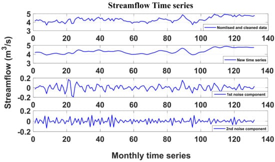
Figure 4.
Normalized and cleaned streamflow time series and the three components obtained by SSA.
Three box plot shapes for normalized, cleaned, and denoised streamflow time series are shown in Figure 5. The figure reveals that the normalized time series had two outliers, and there was no significant difference in the shape of the data compared with the cleaned form. All of the shapes had nearly the same median and upper and lower quartiles, while the upper and lower whiskers of the denoised time series shape were less than those of the other two shapes (normalized and cleaned time series).
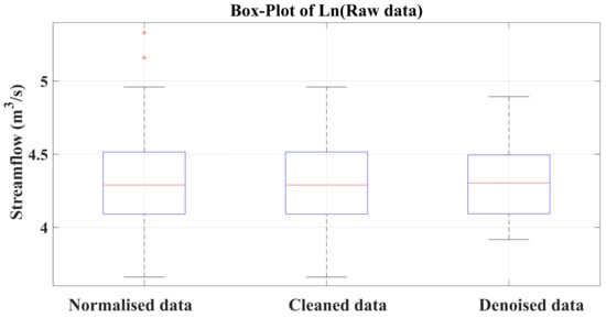
Figure 5.
The normalized, cleaned, and denoised data box plot distribution.
In addition, based on the literature, the first minimum of the average mutual information (AMI) was chosen as the time lag [63,64]. Depending on Figure 6 of AMI, five lags (Lagt_1 to Lagt_5) of monthly historical streamflow data were utilized to estimate future river streamflow.
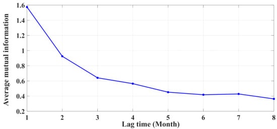
Figure 6.
Average mutual information (AMI) function of the streamflow time series.
According to Zubaidi et al. [47], the relation between sample size (N) and the number of predictor variables (m) should be consistent with Equation (20):
The number of cases in this study was N = 127, which is higher than the required number of 90.
4.2. Model Configuration
After pre-processing processes and analyzing the data, the data were separated into three groups: training, testing, and validation (as previously mentioned in Section 3.2). The ANN model requires integration with the metaheuristic method to establish the ANN model’s optimal hyperparameters (Lr, N1, and N2). As a result, the CPSOCGSA method was combined with the ANN model. The results were then compared to the SMA-ANN and MPA-ANN algorithms for further validation. Swarm sizes of 10, 20, 30, 40, and 50 were used five times, each with 200 iterations for each method in this study in order to obtain the minimal fitness function (MSE). Figure S1 demonstrates an example of the CPSOCGSA-ANN algorithm performance and displays the optimal fitness function for each swarm in terms of the streamflow.
Figure 7A displays that the (30_2) swarm size gave the best solution for the CPSOCGSA-ANN algorithm (MSE = 0.02942, after 179 iterations) for streamflow, while in Figure 7B, the (30_1) swarm size provided the optimal solution for the MPA-ANN algorithm (MSE = 0.03221, after 78 iterations). Figure 7C presents the swarm size (30_1) and offered the best solution for the SMA-ANN algorithm (MSE = 0.03455, after 194 iterations).
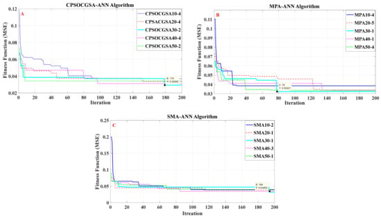
Figure 7.
Fitness function of (A) CPSOCGSA-ANN algorithms, (B) MPA-ANN algorithms, and (C) SMA-ANN algorithms under five swarm sizes.
Consequently, Table 1 shows the ANN hyperparameters for all of the algorithms.

Table 1.
ANN hyperparameters based on the CPSOCGSA-ANN, MPA-ANN, and SMA-ANN algorithms.
4.3. Performance Evaluation
A number of statistical indicators were used to evaluate and compare the performance of the developed techniques (see Section 3.4 for more details). The R2, RMSE, MAE, and MARE of all techniques can be seen in Table 2. A comparison of the findings reveals that all models offered a good forecast level of streamflow time series considering R2, according to Dawson et al. [65]. The CPSOCGSA-ANN and MPA-ANN combined models yielded more accurate findings than the SMA-ANN model based on RMSE, MAE, and MARE (the error values are rescaled). Additionally, the table results confirm that the CPSOCGSA-ANN technique was preferable to other hybrid techniques. A possible explanation for this might be that it is likely related to optimizing the PSO algorithm by GSA, which helps PSO then determine the optimum ANN model’s hyperparameters.

Table 2.
The performance of CPSOCGSA-ANN, MPA-ANN, and SMA-ANN in the validation stage.
Additionally, Figure 8 shows the Taylor diagram for the CPSOCGSA-ANN (B), MPA-ANN (C), and SMA-ANN (D) forecast techniques in the validation stage. This diagram proposes a graphical summary of the agreement between the observed and predicted patterns based on the standard deviation (SD), root-mean-square difference (RMSD), and correlation coefficient (R). In Figure 8, the grey arc, blue azimuthal line, and green contour line refer to values for the SD, R, and RMSD for the observed (reference point, A) pattern, respectively. The diagram reveals that the CPSOCGSA-ANN technique produced low SD, RMSD, and high R, and was the nearest model to the reference point, representing the observed pattern.
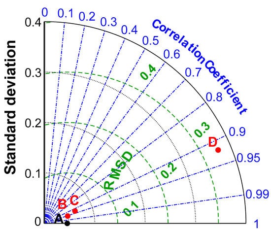
Figure 8.
Taylor diagram for the CPSOCGSA-ANN, MPA-ANN, and SMA-ANN prediction models.
In order to scrutinize the goodness of fit of the three techniques, an error analysis was achieved in the validation stage. The error scatter plots against the sample numbers for the validation stage are presented in Figure 9. What stands out in this figure is that the mean error of the CPSOCGSA-ANN model was closer to zero (from 0.041 to 0.097) than the other techniques, and SMA-ANN was the worst (from −0.874 to 0.375). There was no definite pattern to the distribution. The above outcomes affirmed that the proposed methodology (CPSOCGSA-ANN) offered a more accurate performance than the MPA-ANN and SMA-ANN models.
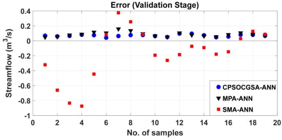
Figure 9.
CPSOCGSA-ANN, MPA-ANN, and SMA-ANN residual scatterplots.
For additional validation of the CPSOCGSA-ANN model, the distribution of the residual data was analyzed. For this, normality tests were used. Shapiro–Wilk and Kolmogorov–Smirnov tests were performed at a significance level of 0.05 to verify or reject the normality of the residual data. The values of both tests were more than 0.05, which means the residual data were normally distributed based on the null hypothesis assumption [66,67]. In addition, the ADF and KPSS tests revealed that the residual data were stationary. Accordingly, these four tests emphasized the capability and reliability of the CPSOCGSA-ANN model.
In addition, a Bland–Altman scatter plot was used to scrutinize the agreement of the CPSOCGSA-ANN model. The plot can show the systematic and random differences and the merit of revealing the variation in the results. Figure 10 shows scattered data, suggesting an excellent distribution fit between limits of agreement (100%). Moreover, a further statistical test revealed that the CPSOCGSA-ANN model yielded SI of 0.015, which indicates an excellent outcome. Taken together, these results indicate the relation between the measured and simulated values.
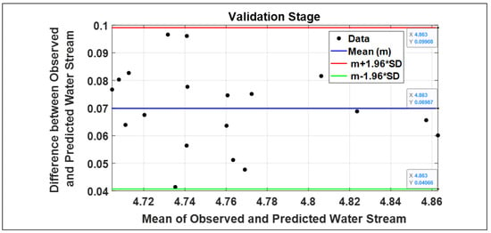
Figure 10.
Bland–Altman plot of the integrated model in the validation stages.
Overall, what stands out in these results is the following:
- (1)
- These results highlight the potential utility of SSA and MI methods for enhancing raw data quality and choosing the best lags scenario without violating the multi-collinearity hypothesis.
- (2)
- CPSOCGSA has been proven to be a reliable algorithm that is applied for integrating the ANN technique for monthly forecast streamflow compared with the SMA and MPA algorithms.
- (3)
- Various statistical analyses have showed that the proposed methodology accurately predicted monthly medium-term streamflow data.
- (4)
- This study reveals the need for further investigation into additional hybrid forecast techniques in different time scales.
5. Conclusions
This study built and examined a novel methodology to forecast the monthly river streamflow based on several previous lags. It employed SSA to denoise raw time series and MI to choose the best predictor scenarios (lags). Additionally, three recent metaheuristic algorithms (CPSOCGSA, MPA, and SMA) were used to integrate the ANN model by determining the optimal hyperparameters. Historical monthly streamflow data of the Tigris River were utilized over 11 years to perform the research. The results of this study identified the significance of data pre-processing techniques for improving the raw data quality and determining the best lags scenario. It has also shown that CPSOCGSA-ANN performed better than the MPA-ANN and SMA-ANN algorithms depending on several statistical criteria, such as R2, RMSE, MAE, and MARE. Taken together, these results reveal that the proposed methodology is a reliable and skillful technique for forecasting monthly streamflow by yielding R2 = 0.91, with an RMSE equal to 1.07 m3/s. These results can offer useful information to the local authorities (i.e., managers and policymakers), helping the irrigation sector company better manage the irrigation system, leading to enhanced service and management of resources in the Maysan Governorate. It is recommended that further research be undertaken in the combined prediction models (HPOH) due to there being an abundance for further progress in pre-treatment signals, data reduction, and for determining machine learning model hyperparameters. In addition, further investigation and experimentation using the combined technique to simulate the streamflow driven by climatic factors are strongly recommended, because extreme weather will likely become more prevalent in the future.
Supplementary Materials
The following supporting information can be downloaded at: https://www.mdpi.com/article/10.3390/hydrology9100171/s1, Figure S1: CPSOCGSA-ANN algorithm performance with five times run for each swarm.
Author Contributions
Conceptualization, S.L.Z.; Data curation, S.L.Z.; Formal analysis, B.A.K. and S.L.Z.; Funding acquisition, N.A.-A.; Methodology, B.A.K., S.L.Z., H.M.R. and N.A.-A.; Project administration, S.L.Z.; Resources, N.A.-A. and N.S.S.A.-B.; Software, H.M.R.; Supervision, S.L.Z.; Validation, B.A.K. and S.L.Z.; Visualization, H.M.R. and N.S.S.A.-B.; Writing—original draft, B.A.K.; Writing—review & editing, B.A.K., S.L.Z. and N.S.S.A.-B. All authors have read and agreed to the published version of the manuscript.
Funding
This research received no external funding.
Data Availability Statement
Data were provided by the Directorate of Water Resources in Maysan City.
Conflicts of Interest
The authors declare no conflict of interest.
References
- Ahmadi, M.S.; Sušnik, J.; Veerbeek, W.; Zevenbergen, C. Towards a global day zero? Assessment of current and future water supply and demand in 12 rapidly developing megacities. Sustain. Cities Soc. 2020, 61, 102295. [Google Scholar] [CrossRef]
- He, C.; Liu, Z.; Wu, J.; Pan, X.; Fang, Z.; Li, J.; Bryan, B.A. Future global urban water scarcity and potential solutions. Nat. Commun. 2021, 12, 4667. [Google Scholar] [CrossRef] [PubMed]
- Zhang, X.; Chen, N.; Sheng, H.; Ip, C.; Yang, L.; Chen, Y.; Sang, Z.; Tadesse, T.; Lim, T.P.Y.; Rajabifard, A.; et al. Urban drought challenge to 2030 sustainable development goals. Sci. Total Environ. 2019, 693, 133536. [Google Scholar] [CrossRef] [PubMed]
- Rajarethinam, K.; Varuvel, D.; Bagodi, V. System dynamic modelling for assessing the vulnerability of water resources: A case of Chennai City, Tamil Nadu, India. Arab. J. Geosci. 2021, 14, 2008. [Google Scholar] [CrossRef]
- Ethaib, S.; Zubaidi, S.L.; Al-Ansari, N.; Fegade, S.L. Evaluation water scarcity based on GIS estimation and climate-change effects: A case study of Thi-Qar Governorate, Iraq. Cogent Eng. 2022, 9, 2075301. [Google Scholar] [CrossRef]
- Salman, S.A.; Shahid, S.; Ismail, T.; Chung, E.-S.; Al-Abadi, A.M. Long-term trends in daily temperature extremes in Iraq. Atmos. Res. 2017, 198, 97–107. [Google Scholar] [CrossRef]
- Osman1, Y.; Abdellatif2, M.; Al-Ansari3, N.; Knutsson4, S.; Jawad, S. Climate Change And Future Precipitation In An Arid Environment Of The Middle East: Case Study Of Iraq. J. Environ. Hydrol. 2017, 25, 3. [Google Scholar]
- Han, K.; Wang, Y. A review of artificial neural network techniques for environmental issues prediction. J. Therm. Anal. Calorim. 2021, 145, 2191–2207. [Google Scholar] [CrossRef]
- Hu, H.; Zhang, J.; Li, T. A Novel Hybrid Decompose-Ensemble Strategy with a VMD-BPNN Approach for Daily Streamflow Estimating. Water Resour. Manag. 2021, 35, 5119–5138. [Google Scholar] [CrossRef]
- Li, F.-F.; Wang, Z.-Y.; Zhao, X.; Xie, E.; Qiu, J. Decomposition-ANN Methods for Long-Term Discharge Prediction Based on Fisher’s Ordered Clustering with MESA. Water Resour. Manag. 2019, 33, 3095–3110. [Google Scholar] [CrossRef]
- Wegayehu, E.B.; Muluneh, F.B. Multivariate Streamflow Simulation Using Hybrid Deep Learning Models. Comput. Intell. Neurosci. 2021, 2021, 5172658. [Google Scholar] [CrossRef] [PubMed]
- Zhang, Z.; Zhang, Q.; Singh, V.P. Univariate streamflow forecasting using commonly used data-driven models: Literature review and case study. Hydrol. Sci. J. 2018, 63, 1091–1111. [Google Scholar] [CrossRef]
- Meshram, S.G.; Meshram, C.; Santos, C.A.G.; Benzougagh, B.; Khedher, K.M. Streamflow Prediction Based on Artificial Intelligence Techniques. Iran. J. Sci. Technol. Trans. Civ. Eng. 2021, 46, 2393–2403. [Google Scholar] [CrossRef]
- Deka, S.K.P.C. Performance enhancement of SVM model using discrete wavelet transform for daily streamflow forecasting. Environ. Earth Sci. 2021, 80, 101. [Google Scholar] [CrossRef]
- Vatanchi, S.M.; Etemadfard, H.; Maghrebi, M.F.; Shad, R. A Comparative Study on Forecasting of Long-term Daily Streamflow using ANN, ANFIS, BiLSTM, and CNN-GRU-LSTM. Search Life-Sci. Lit. 2022; preprint. [Google Scholar] [CrossRef]
- Peng, T.; Zhou, J.; Zhang, C.; Fu, W. Streamflow Forecasting Using Empirical Wavelet Transform and Artificial Neural Networks. Water 2017, 9, 406. [Google Scholar] [CrossRef]
- Kilinc, H.C.; Haznedar, B. A Hybrid Model for Streamflow Forecasting in the Basin of Euphrates. Water 2022, 14, 80. [Google Scholar] [CrossRef]
- Md. Munir Hayet Khan, N.S.M.; El-Shafie, A. Wavelet based hybrid ANN-ARIMA models for meteorological drought forecasting. J. Hydrol. 2020, 590, 125380. [Google Scholar] [CrossRef]
- Fathian, F.; Mehdizadeh, S.; Kozekalani Sales, A.; Safari, M.J.S. Hybrid models to improve the monthly river flow prediction: Integrating artificial intelligence and non-linear time series models. J. Hydrol. 2019, 575, 1200–1213. [Google Scholar] [CrossRef]
- Wang, Z.; Fathollahzadeh Attar, N.; Khalili, K.; Behmanesh, J.; Band, S.S.; Mosavi, A.; Chau, K.-W. Monthly streamflow prediction using a hybrid stochastic-deterministic approach for parsimonious non-linear time series modeling. Eng. Appl. Comput. Fluid Mech. 2020, 14, 1351–1372. [Google Scholar] [CrossRef]
- Zainab Abdulelah Al Sudani, S.Q.S.; Sharafati, A.; Mundher, Z.; Yaseen, Z.M. Development of multivariate adaptive regression spline integrated with differential evolution model for streamflow simulation. J. Hydrol. 2019, 573, 1–12. [Google Scholar] [CrossRef]
- Pham, Q.B.; Afan, H.A.; Mohammadi, B.; Ahmed, A.N.; Linh, N.T.T.; Vo, N.D.; Moazenzadeh, R.; Yu, P.-S.; El-Shafie, A. Hybrid model to improve the river streamflow forecasting utilising multi-layer perceptron-based intelligent water drop optimisation algorithm. Soft Comput. 2020, 24, 18039–18056. [Google Scholar] [CrossRef]
- Zubaidi, S.L.; Gharghan, S.K.; Dooley, J.; Alkhaddar, R.M.; Abdellatif, M. Short-Term Urban Water Demand Prediction Considering Weather Factors. Water Resour. Manag. 2018, 32, 4527–4542. [Google Scholar] [CrossRef]
- Zubaidi, S.L.; Kot, P.; Alkhaddar, R.M.; Abdellatif, M.; Al-Bugharbee, H. Short-Term Water Demand Prediction in Residential Complexes: Case Study in Columbia City, USA. In Proceedings of the 11th International Conference on Developments in eSystems Engineering (DeSE), Cambridge, UK, 2–5 September 2018; pp. 31–35. [Google Scholar]
- Ouyang, Q.; Lu, W. Monthly Rainfall Forecasting Using Echo State Networks Coupled with Data Preprocessing Methods. Water Resour. Manag. 2017, 32, 659–674. [Google Scholar] [CrossRef]
- Zhao, X.; Lv, H.; Lv, S.; Sang, Y.; Wei, Y.; Zhu, X. Enhancing robustness of monthly streamflow forecasting model using gated recurrent unit based on improved grey wolf optimizer. J. Hydrol. 2021, 601, 126607. [Google Scholar] [CrossRef]
- Apaydin, H.; Sattari, M.T.; Falsafian, K.; Prasad, R. Artificial intelligence modelling integrated with Singular Spectral analysis and Seasonal-Trend decomposition using Loess approaches for streamflow predictions. J. Hydrol. 2021, 600, 126506. [Google Scholar] [CrossRef]
- Huang, S.; Chang, J.; Huang, Q.; Chen, Y. Monthly streamflow prediction using modified EMD-based support vector machine. J. Hydrol. 2014, 511, 764–775. [Google Scholar] [CrossRef]
- Niu, W.-J.; Feng, Z.-K.; Yang, W.-F.; Zhang, J. Short-term streamflow time series prediction model by machine learning tool based on data preprocessing technique and swarm intelligence algorithm. Hydrol. Sci. J. 2020, 65, 2590–2603. [Google Scholar] [CrossRef]
- Jiang, Y.; Bao, X.; Hao, S.; Zhao, H.; Li, X.; Wu, X. Monthly Streamflow Forecasting Using ELM-IPSO Based on Phase Space Reconstruction. Water Resour. Manag. 2020, 34, 3515–3531. [Google Scholar] [CrossRef]
- Maier, H.R.; Jain, A.; Dandy, G.C.; Sudheer, K.P. Methods used for the development of neural networks for the prediction of water resource variables in river systems: Current status and future directions. Environ. Model. Softw. 2010, 25, 891–909. [Google Scholar] [CrossRef]
- Ibrahim, K.S.M.H.; Huang, Y.F.; Ahmed, A.N.; Koo, C.H.; El-Shafie, A. A review of the hybrid artificial intelligence and optimisation modelling of hydrological streamflow forecasting. Alex. Eng. J. 2021, 61, 279–303. [Google Scholar] [CrossRef]
- Şenel, F.A.; Gökçe, F.; Yüksel, A.S.; Yiğit, T. A novel hybrid PSO–GWO algorithm for optimization problems. Eng. Comput. 2018, 35, 1359–1373. [Google Scholar] [CrossRef]
- Wolpert, D.H.; Macready, W.G. No free lunch theorems for optimization. IEEE Trans. Evol. Comput. 1997, 1, 67–82. [Google Scholar] [CrossRef]
- Candelieri, A. Clustering and Support Vector Regression for Water Demand Forecasting and Anomaly Detection. Water 2017, 9, 224. [Google Scholar] [CrossRef]
- Li, S.; Chen, H.; Wang, M.; Heidari, A.A.; Mirjalili, S. Slime mould algorithm: A new method for stochastic optimisation. Future Gener. Comput. Syst. 2020, 111, 300–323. [Google Scholar] [CrossRef]
- Kumar, C.; Raj, T.D.; Premkumar, M.; Raj, T.D. A new stochastic slime mould optimisation algorithm for the estimation of solar photovoltaic cell parameters. Optik 2020, 223, 165277. [Google Scholar] [CrossRef]
- Fan, Q.; Huang, H.; Chen, Q.; Yao, L.; Yang, K.; Huang, D. A modified self-adaptive marine predators algorithm: Framework and engineering applications. Eng. Comput. 2021, 38, 3269–3294. [Google Scholar] [CrossRef]
- Eid, A.; Kamel, S.; Abualigah, L. Marine predators algorithm for optimal allocation of active and reactive power resources in distribution networks. Neural Comput. Appl. 2021, 33, 14327–14355. [Google Scholar] [CrossRef]
- Rather, S.A.; Bala, P.S. Hybridization of Constriction Coefficient-Based Particle Swarm Optimization and Chaotic Gravitational Search Algorithm for Solving Engineering Design Problems. In Applied Soft Computing and Communication Networks; Springer: Singapore, 2020; Volume 125, pp. 95–115. [Google Scholar]
- Eiben, A.E.; Schippers, C.A. On evolutionary exploration and exploitation. Fundam. Inform. 1998, 35, 35–50. [Google Scholar] [CrossRef]
- Hajirahimi, Z.; Khashei, M. Hybridization of hybrid structures for time series forecasting: A review. Artif. Intell. Rev. 2022, in press. [Google Scholar] [CrossRef]
- Magali Troin, R.A.; Andrew, W. Wood, François Brissette, and; Martel, J.-L. Generating Ensemble Streamflow Forecasts: A Review of Methods and Approaches Over the Past 40 Years. Water Resour. Res. 2021, 57, 1–48. [Google Scholar] [CrossRef]
- Tao, H.; Al-Sulttani, A.O.; Salih Ameen, A.M.; Ali, Z.H.; Al-Ansari, N.; Salih, S.Q.; Mostafa, R.R.; Shahid, S. Training and Testing Data Division Influence on Hybrid Machine Learning Model Process: Application of River Flow Forecasting. Complexity 2020, 2020, 8844367. [Google Scholar] [CrossRef]
- Abood, R.H.; Mahmoud, R.R. Drought Assessment Using Gis And Meteorological Data In Maysan Province /Iraq. Int. J. Civ. Eng. Technol. 2018, 9, 516–524. [Google Scholar]
- Saleh, A.M. Improving the Accuracy of Land Cover Classification using Sentinel 2 Data and Knowledge Based Classification System in the West of Amara City, Iraq. J. Indian Soc. Soil Sci. 2022, 70, 1–9. [Google Scholar] [CrossRef]
- Zubaidi, S.L.; Ortega-Martorell, S.; Al-Bugharbee, H.; Olier, I.; Hashim, K.S.; Gharghan, S.K.; Kot, P.; Alkhaddar, R.M. Urban Water Demand Prediction for a City That Suffers from Climate Change and Population Growth: Gauteng Province Case Study. Water 2020, 12, 1885. [Google Scholar] [CrossRef]
- Hassani, H. Singular spectrum analysis: Methodology and comparison. J. Data Sci. 2007, 5, 239–257. [Google Scholar] [CrossRef]
- Pham, Q.B.; Yang, T.-C.; Kuo, C.-M.; Tseng, H.-W.; Yu, P.-S. Coupling Singular Spectrum Analysis with Least Square Support Vector Machine to Improve Accuracy of SPI Drought Forecasting. Water Resour. Manag. 2021, 35, 847–868. [Google Scholar] [CrossRef]
- Al-Bugharbee, H.; Trendafilova, I. A Fault Diagnosis Methodology for Rolling Element Bearings Based on Advanced Signal Pretreatment And Autoregressive Modelling. J. Sound Vib. 2016, 369, 246–265. [Google Scholar] [CrossRef]
- Zhigljavsky, A. Singular spectrum analysis for time series: Introduction to this special issue. Stat. Its Interface 2010, 3, 255–258. [Google Scholar] [CrossRef]
- Danandeh Mehr, A.; Ghadimi, S.; Marttila, H.; Torabi Haghighi, A. A new evolutionary time series model for streamflow forecasting in boreal lake-river systems. Theor. Appl. Climatol. 2022, 148, 255–268. [Google Scholar] [CrossRef]
- Barzegar, R.; Adamowski, J.; Moghaddam, A.A. Application of wavelet-artificial intelligence hybrid models for water quality prediction: A case study in Aji-Chay River, Iran. Stoch. Environ. Res. Risk Assess. 2016, 30, 1797–1819. [Google Scholar] [CrossRef]
- Abbaa, S.I.; Hadia, S.J.; Abdullahi, J. River water modelling prediction using multi-linear regression, artificial neural network, and adaptive neuro-fuzzy inference system techniques. Procedia Comput. Sci. 2017, 120, 75–82. [Google Scholar] [CrossRef]
- Tiu, E.S.K.; Huang, Y.F.; Ng, J.L.; AlDahoul, N.; Ahmed, A.N.; Elshafie, A. An evaluation of various data pre-processing techniques with machine learning models for water level prediction. Nat. Hazards 2021, 110, 121–153. [Google Scholar] [CrossRef]
- Bayatvarkeshi, M.; Mohammadi, K.; Kisi, O.; Fasihi, R. A new wavelet conjunction approach for estimation of relative humidity: Wavelet principal component analysis combined with ANN. Neural Comput. Appl. 2018, 32, 4989–5000. [Google Scholar] [CrossRef]
- Thomas, A.J.; Petridis, M.; Walters, S.D.; Gheytassi, S.M.; Morgan, R.E. Two Hidden Layers are Usually Better than One. In Engineering Applications of Neural Networks; Springer: Berlin/Heidelberg, Germany, 2017; Volume 744, pp. 279–290. [Google Scholar]
- Farzad, F.; El-Shafie, A.H. Performance enhancement of rainfall pattern–water level prediction model utilizing self-organizing-map clustering method. Water Resour. Manag. 2017, 31, 945–959. [Google Scholar] [CrossRef]
- González Perea, R.; Camacho Poyato, E.; Montesinos, P.; Rodríguez Díaz, J.A. Optimisation of water demand forecasting by artificial intelligence with short data sets. Biosyst. Eng. 2019, 177, 59–66. [Google Scholar] [CrossRef]
- Maurice Clerc, J.K. The Particle Swarm—Explosion, Stability, and Convergence in a Multidimensional Complex Space. IEEE Trans. Evol. Comput. 2002, 6, 58–73. [Google Scholar] [CrossRef]
- Khajehzadeh, M.; Taha, M.R.; Eslami, M. Efficient gravitational search algorithm for optimum design of retaining walls. Struct. Eng. Mech. 2013, 45, 111–127. [Google Scholar] [CrossRef]
- Rather, S.A.; Bala, P.S. Hybridisation of constriction coefficient based particle swarm optimisation and gravitational search algorithm for function optimisation. In Proceedings of the International Conference on Advances in Electronics, Electrical & Computational Intelligence (ICAEEC), Prayagraj, India, 31 May–1 June 2019. [Google Scholar]
- Stergiou, N. Nonlinear Analysis for Human Movement Variability; CRC Press: Boca Raton, FL, USA, 2016. [Google Scholar]
- Aldrich, C.; Auret, L. Unsupervised Process Monitoring and Fault Diagnosis with Machine Learning Methods; Springer: Berlin/Heidelberg, Germany, 2013. [Google Scholar]
- Dawson, C.W.; Abrahart, R.J.; See, L.M. HydroTest: A web-based toolbox of evaluation metrics for the standardised assessment of hydrological forecasts. Environ. Model. Softw. 2007, 22, 1034–1052. [Google Scholar] [CrossRef]
- Tabachnick, B.G.; Fidell, L.S.; Ullman, J.B. Using Multivariate Statistics; Pearson: Boston, MA, USA, 2007; Volume 5. [Google Scholar]
- Valentini, M.; Dos Santos, G.B.; Vieira, B.M. Multiple linear regression analysis (MLR) applied for modeling a new WQI equation for monitoring the water quality of Mirim Lagoon, in the state of Rio Grande do Sul—Brazil. SN Appl. Sci. 2021, 3, 70. [Google Scholar] [CrossRef]
Publisher’s Note: MDPI stays neutral with regard to jurisdictional claims in published maps and institutional affiliations. |
© 2022 by the authors. Licensee MDPI, Basel, Switzerland. This article is an open access article distributed under the terms and conditions of the Creative Commons Attribution (CC BY) license (https://creativecommons.org/licenses/by/4.0/).