1. Introduction
In recent decades, population growth, industrialization, and urbanization have generated an ever-increasing demand for fresh water [
1,
2,
3]. This has led to a huge transition from small and local water resource exploitation and distribution networks to regional and more integrated systems that bring water from springs and wells over great distances.
Traditionally, areas on the Mediterranean, specifically Central Italy, sourced water from local small springs or wells near villages and towns [
4]. Now, water for drinking, irrigation, hydroelectricity production, and manufacturing mainly come from regional karst or alluvial aquifers [
5,
6,
7,
8,
9,
10,
11]. As a matter of fact, the regular steady baseflow of springs and rivers is directly connected to the amount of groundwater [
12].
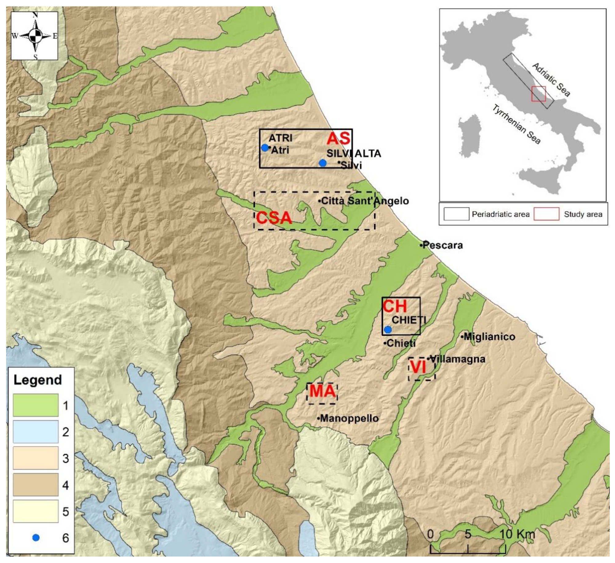
The principal aqueducts, which have a capillary pipeline system on the order of hundreds of kilometers, distribute groundwater to both the Tyrrhenian and Adriatic coasts (
Figure 1) mainly from the karst aquifers in the Apennine Mountains [
13,
14,
15,
16] and to a lesser extent from alluvial aquifers [
17,
18,
19,
20,
21].
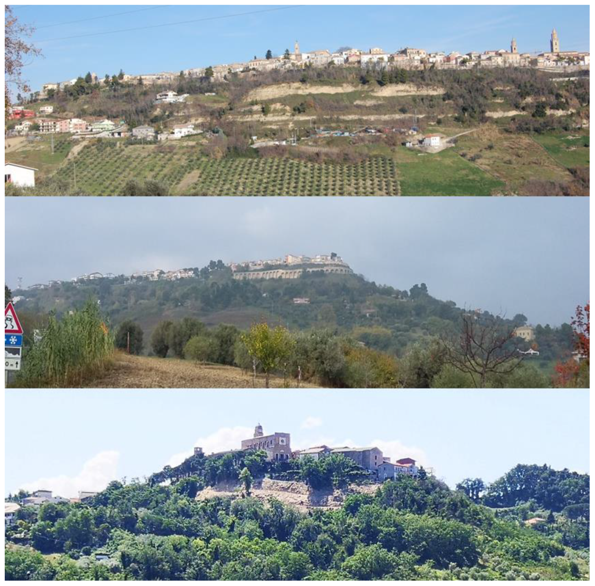
The abovementioned economic transition caused a progressive abandonment of local aquifers located in the terrigenous sandy and gravelly stratigraphic sequence that constitutes the top of important hills in the Periadriatic area. Here, springs and elevated flat plains bounded by steep slopes provided optimal topographical and morphological conditions for the development of towns (
Figure 2) that played an important political and commercial role a few centuries ago [
22].
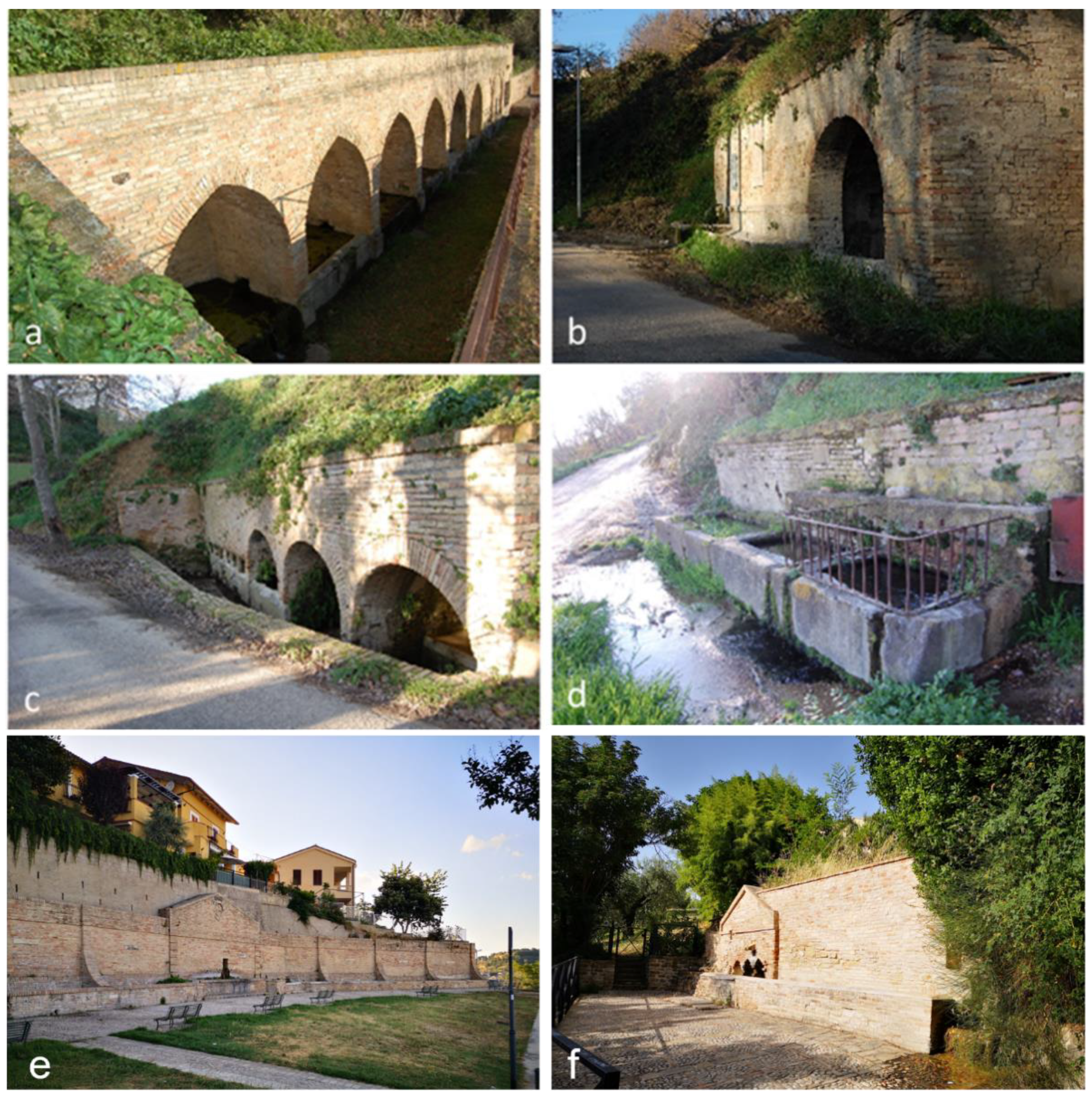
Until the middle of the 20th century, these springs were the sole source of freshwater (
Figure 3), and local communities used peculiar water-tapping systems consisting of a combination of drainage tunnels and wells located at the interface between permeable and non-permeable geological bodies. Springs’ discharge is rarely over 1 L/s and usually it goes from 0.1 to 0.4 L/s during summer and from 0.3 and 0.9 L/s during winter. These systems are similar to the Persian “Quanats”, as they had similar hydraulic functions (i.e., draining water from subsoil). Different archaeological studies have investigated these water-tapping systems [
22,
23], pointing out that, besides being able to extract groundwater, they also served as protective barriers against pollution and high temperatures that could cause rapid evaporation.
The geological features of these water bodies have already been investigated in many detailed studies either from a stratigraphic and sedimentological [
24,
25] or paleoenvironmental point of view and as on-shore and off-shore natural gas reservoirs [
26,
27]. Nevertheless, the hydrogeological features of these local aquifers are unclear. In fact, no detailed investigation has been conducted on their geometries: groundwater flow, physico-chemical properties, and quantification of stored water volumes and seasonal recharge. Such information would be highly valuable because water from secondary sources like local groundwater could help mitigate water scarcity and the overexploitation of larger water distribution networks, worsened by drought periods caused by climate change [
28,
29,
30,
31].
For these reasons, this study’s objective was twofold: to characterize the hydrodynamic and hydrochemical properties of five sample aquifers (
Figure 1) and to quantify the “groundwater budget”, the seasonal recharge and total amount stored in the subsoil.
It is worth noting that, except for restricted use for recreational purposes, these wells and springs fell into disuse because of urban development, the spread of water networks, and the loss of surrounding farmland, so the opportunity for a detailed study based on continuous monitoring has been very limited.
In fact, the only available method was manual seasonal monitoring through a field survey of a few accessible wells (usually private) and well-known springs. For this reason, the observational data in this study represent an informative hydrogeological scenario that is often the only one available for aquifer management. Recharge estimation for this kind of aquifer was carried out by calculating the yearly specific recharge (Mm3/y/km2) in the five areas using different methods: (1) a water budget starting from weather data, rainfall, and temperature; (2) water table fluctuation measured seasonally in wells; and (3) a water budget based on spring water discharge.
The paper first explains the methods used, then characterizes the five sites from a geological and hydrogeological point of view; after this, the data are shown in a table and charts, followed by a discussion of the results and conclusions.
2. Materials and Methods
2.1. Study Area
The five study areas are in the hilly Periadriatic region in Central Italy at elevations up to 300 m above sea level (a.s.l.); they are, from north to south, Atri and Silvi (AS), Città Sant’Angelo (CSA), Chieti (CH), Villamagna (VI), and Manoppello (MA) (
Figure 1).
These were chosen because of the importance of the old city centers, for the historical and evident aqueducts and for the available literature information about water uses. Geologically speaking, all are characterized by foredeep deposits (Plio-Pleistocene age). The soil is mainly marly-clayey, with a coarsening upward trend in the upper portion where an arenaceous lithology can be found. These deposits are known as the Mutignano Formation [
32,
33] and three associations can be observed from bottom to top:
- -
Marly-clayey (clays and marly-clayey deposits with sandy levels);
- -
Sandy-clayey, (sands and clayey sands); and
- -
Sandy-gravelly (arenaceous deposits with gravelly levels in the upper portion,
Figure 4).
However, above the Mutignano Formation, continental deposits are found, mainly alluvial (sands and gravels) and slope deposits (mix of sands, gravels, and silts).
From now on, sandy-gravel and sandy-clayey will be associated in the “arenaceous complex” because of their similar properties, while the marly-clayey association will be considered as the “clayey complex”.
The geomorphology of the landscape is related to the outcroppings of arenaceous deposits having a flat shape and subvertical slopes as boundaries, which at the base are less steep.
The hydrogeological features of these aquifers are influenced by stratigraphic ones [
34]. As a result, an aquifer was found inside the arenaceous complex, while the clay complex is individuated as aquiclude [
35]. The hydraulic conductivity of the porous lithotypes (associations) constituting these aquifers, estimated from previous works by a pumping test in similar lithologies [
18,
19,
20,
36,
37], is marly-clayey, 10
−8 < K < 10
−6; sandy-clayey, 10
−5 < K < 10
−3; and sandy-gravelly, ~10
−3 m/s, in addition to the highly variable values (10
−8 < K < 10
−4 m/s) of the continental deposits.
At the interface between the arenaceous and the clayey complexes, springs were found, whose groundwater had often been exploited by complex systems of wells and drainage tunnels (
Figure 3).
2.2. Datasets
Different kinds of data were used to characterize the hydrodynamic features of the arenaceous hilly aquifers and to quantify with a certain degree of confidence the groundwater resources of these secondary water bodies. Weather data (i.e., monthly rainfall and temperature) collected at the monitoring stations were considered for estimating the effective infiltration (
Table 1).
Seasonal variation in groundwater was assessed by measuring the hydraulic head of wells and spring discharges (
Table 2) during both the wet and dry seasons.
Groundwater physico-chemical parameters (temperature, electrical conductivity, pH, and redox potential) were measured in the abovementioned monitoring network for thorough aquifer characterization and to acquire deeper insight into the recharge mechanism.
2.3. Yearly Specific Recharge
As pointed out in the previous section, single aquifers are characterized by different sizes. For this reason, to compare the recharge and the water budget, the yearly specific recharge was considered as a reference recharge unit (i.e., all results were converted to this unit after calculation). This defined the water volume in millions of cubic meters that infiltrates yearly per square kilometer (i.e., Mm
3/y/km
2) and was calculated through the three different approaches described below, to provide a recharge estimation that was as exhaustive and representative as possible. The extension of the recharging area was calculated based on the outcrop area of the arenaceous complex (n. 3 and 4 in the geological map and cross-section of
Figure 5 and
Figure 6). In this sense, the vertical variation of the piezometric surface does not involve variations in the extension of the recharge area.
2.3.1. Recharge Estimation from Weather Data
The yearly water budget for aquifer recharge is defined as:
where
is the aquifer recharge,
is the total rainfall related to a certain area, and
is real evapotranspiration, while
is the infiltration rate, which depends on the actual vertical hydraulic conductivity of aquifers in the recharge areas.
Most of this water budget is based on
, which in this study was calculated using two methods: the Turc [
38] and the Thornthwaite and Mather [
39]. Both provided mean real evapotranspiration values related to a statistically significant period (i.e., over at least 30 years), which can be assumed as representative of the local meteo-climatic condition.
The Turc method allowed for a yearly estimate of the
value through the following relation in Equation (2):
where
is the evaporative potential of the atmosphere
, and
is the mean yearly temperature of air (°C). This is the simpler of the two methods for quantifying evapotranspiration because it does not consider seasonal variation in the total amount of water returned to the atmosphere either to affect air temperature (evaporation), or for plant life and growth (transpiration).
A more accurate estimation is provided by the method proposed by Thornthwaite and Mather [
39], which calculates potential evapotranspiration in relation to the ith month
through an exponential equation (Equation (3)):
where
is a corrective coefficient for the latitude;
is the air temperature related to the
ith month (in °C); and
is the exponent of Equation (3), which is based on the yearly heat index
.
Monthly values were compared with the residual water content within the shallower portion of the soil, where plant roots influence the water budget, to estimate the monthly evapotranspiration values (). In this way, the yearly value was estimated while considering the seasonal variability and the actual availability of water in the topsoil.
After calculating the amount of water returning to the atmosphere, the recharge was calculated accordingly to Equation (1). The lithotype of the aquifers under investigation were sandy deposits with a variable amount of fine-sized fraction; thus, the corresponding
values ranged between 0.4 and 0.6 [
36].
2.3.2. Recharge Estimation from Water Level Fluctuation
The second method used to quantify the yearly specific recharge was based on water table fluctuation, which is considered to be almost completely dependent of rainfall infiltration. Considering the difference between the hydraulic head measurements related to the dry and wet seasons
, the effective porosity
of lithotypes forming the aquifers, and the recharge areas
, water recharge volumes
were calculated as follows:
Taking into account the saturated portions of each aquifer instead of , the total amount of groundwater stored in each season was also estimated, providing a more thorough quantification of the water resource.
The
values used in Equation (4) were estimated through pumping tests performed on four wells in some of the aquifers (
Figure 5 and
Figure 6). These tests were carried out with very low flow rates (~0.5–1 L/s) and lasted 6–7 h (including both the pumping and recovery phases). From an analytical point of view, the Cooper–Jacob method [
40], a simplification of the Theis theory [
41], was selected to estimate the p
e values (Method 1). This approach allowed calculation of the storativity (
, unitless) by Equation (5) and data from the pumping phase, which corresponds to the effective porosity for an unconfined aquifer, like those under investigation (i.e.,
:
where
is the intercept initial time (s) at drawdown equal to zero;
is the well radius (m); and
is transmissivity (m
2/s) obtained by the following equation:
where
Q is the constant pumping rate (m
3/s), and
is a coefficient depending on the hydraulic head variation
, taking place in the time interval between
and
.
Besides calculating for yearly specific recharge estimations, hydraulic conductivity values (m/s) were obtained from transmissivity values to provide additional quantitative information about the hydrodynamics of the aquifers.
Tests were carried out in quasi-ideal conditions, as equilibrium during the pumping phase had not been achieved properly; however, the results were reliable because the test data were analyzed by other methods for cross-checking. More specifically,
values were also calculated by applying Equations (5) and (6) to the data from the recovery phase (Method 2), and the Theis method to data from both the pumping and recovery phases (Method 3), which give transmissivity values as follows:
where
is the residual drawdown.
2.3.3. Recharge Estimation from Total Discharge
The last approach to estimating the yearly specific recharge related to the five aquifers was based on direct measurement of their total discharge, which is mainly due to the springs that form at the interface between the arenaceous complex and the underlying marly-clayey aquiclude. Given the hydrodynamic features of this kind of aquifer, the water volumes discharging at the boundaries were definitely considered to be the recharge water that infiltrated and then almost completely comes out every year. This quantity of groundwater, if extrapolated over a year (Mm3/y), can be easily converted into a yearly specific recharge by dividing it by the recharge area, which is known with a high level of confidence. However, this method, although hypothetically the most realistic, is affected by a lack of information about the amount of groundwater flowing toward the surface water bodies through the soil or surficial alteration of impervious lithotypes (i.e., the marly-clayey aquitard), or discharging on the surface and then directly evapotraspirating into the atmosphere.
3. Results and Discussion
3.1. Aquifer Characterization
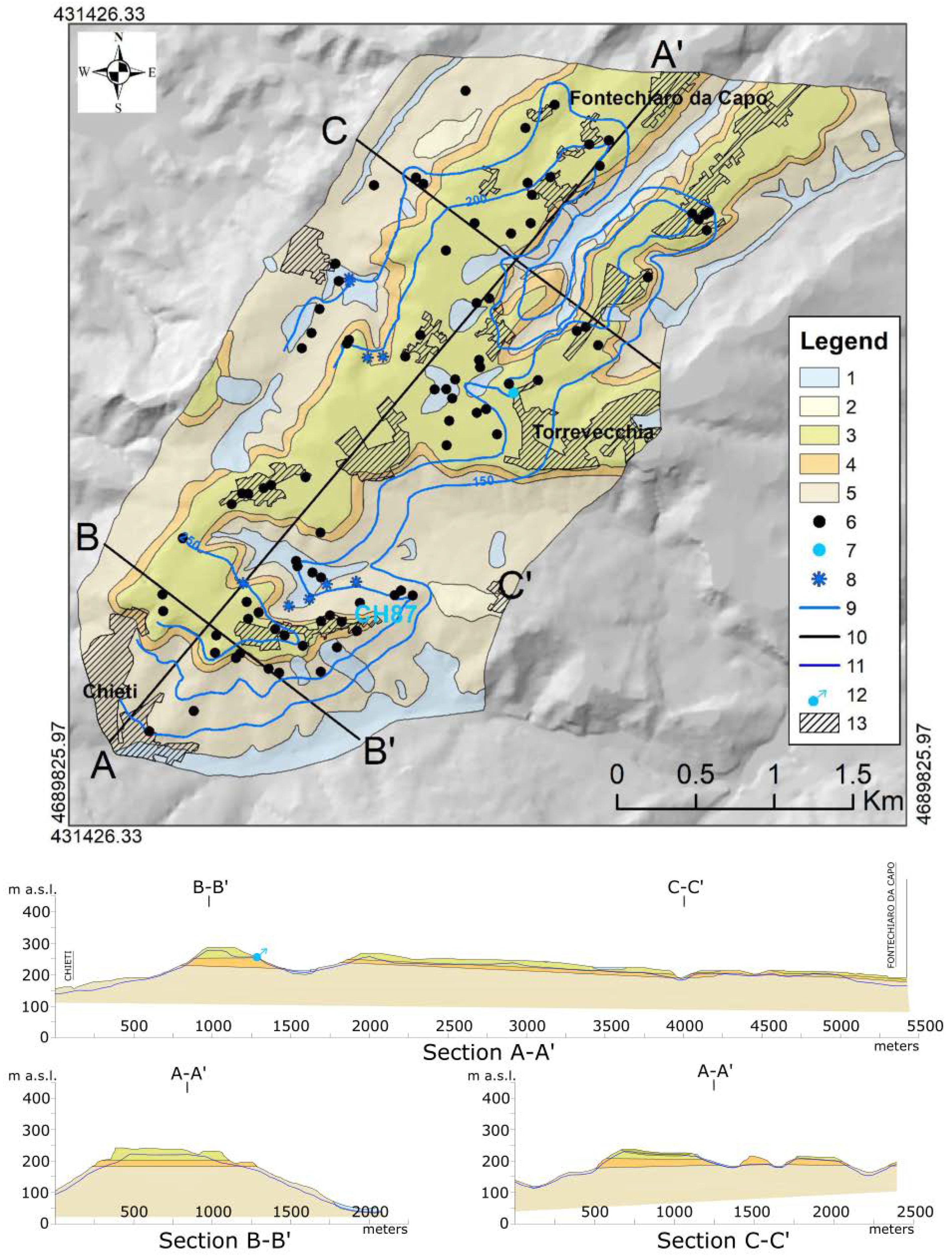
An aquifer characterization was carried out for all five areas; however, only the results for CH and AS will be shown in detail in the text (
Figure 5 and
Figure 6).
In all areas, the stratification is horizontal, and the arenaceous complex (i.e., the sandy-gravelly and sandy-clayey associations together) is some tens of meters thick, while the clayey one is over 500 m. The alluvial deposits can be found in the valleys where the arenaceous complex was eroded, and local streams and rivers deposited a mix of gravelly, sandy, and silty deposits.
The hydraulic head distribution was reconstructed inside the arenaceous complex using the measurements collected in the wells (
Figure 5 and
Figure 6). Occasionally, the water table contours can also be found in the clayey complex, because of secondary hydraulic conductivity related to the clay alteration.
As can be seen from the cross-sections in
Figure 5 and
Figure 6, the arenaceous complex acts as an aquifer, while the clayey complex acts as an aquiclude or sometimes as an aquitard. The maximum thickness of the aquifer in each area varies from a few tens of meters to about 200 m, while the maximum saturated thickness varies from a few to tens of meters. Generally, only the shallower portion of the most permeable complex (i.e., the sandy-gravelly association) was tapped by the historical systems (
Figure 3), and today it is exploited by wells in the urban area. This portion of the aquifer is also characterized by the lowest hydraulic gradients. Moving towards the edges of the plateaus and therefore towards the hydraulic boundary between the arenaceous and clayey complexes, the gradients tend to increase due to a considerable decrease in hydraulic conductivity. In general, groundwater moves from higher aquifer portions to lower ones; thus, in all areas, the groundwater flow is divergent. Furthermore, when an underground drainage axis is present, flowlines converge; usually, these drainage axes correspond to surface valleys.
Analyzing the physico-chemical properties of groundwater flowing into these aquifers (
Table 3 and
Table 4), it appears that the pH values range between 7 and 8 in each studied area and in both summer and winter. This evidence shows the groundwater is slightly alkaline. The electrical conductivity values vary from about 600 to about 1120 µS/cm. Looking at water temperature, the groundwater is generally below 20 °C; thus, the waters can be considered cold [
36]. Finally, an oxidizing environment was found by redox potential in all sampling areas.
A comparison of
Table 3 and
Table 4 shows that the aquifer recharge that take place during the winter and spring has a significant effect, especially on temperature and redox potentials; however, it is quite unclear for electrical conductivity and pH. In fact, the cold oxygenated water infiltrating during winter decreases the groundwater temperature and at the same time increases considerably the redox potential for all the aquifers. The unclear results of the electrical conductivity and pH measurements could be attributed to the fact that these physico-chemical parameters are strongly influenced by a multitude of processes that affect the total salinity and the acidity of groundwater. Moreover, potential human contaminations cannot be excluded [
42], independently from season, due to the presence of an aqueduct, sewer, and farming areas where chemical treatments are operated.
3.2. Recharge Estimation from Weather Data
The water budgets in the AS and CH areas were calculated using monthly rainfall and temperature collected at the gauging stations shown in
Figure 1 and
Table 2.
In both areas, during a warm and dry summer, the average air temperature is about 24 °C and precipitation is in the range 34–41 mm, whereas they are 6 °C and 85–100 mm, respectively, during winter.
For comparison, the water balance for areas AS, CH, and VI was also calculated, based on weather data corresponding to the monitoring period. All the results are shown in
Table 5.
According to previous water budget calculations in the same area [
17,
20,
36,
43], the estimated outflow is 25–30% of the measured rainfall.
Table 6 and
Table 7 show the yearly specific recharge values corresponding to the water budget calculated using both historical and weather data from the monitoring period.
As can be seen from
Table 6 and
Table 7, the yearly specific recharge for the historical period is quite similar to the one for the monitoring period. However, in the AS area, a difference was seen: the outflow seems to be considerably higher for the monitoring period, which led to a higher yearly specific recharge. This could have been caused by greater precipitation than those observed during the historical period.
As expected, the results show a clear dependance on rainfall. Although the monitoring period is one year or a few, the rainfall and yearly specific recharge are similar (
Table 7). In any case, the recharge values are always over 0.1 Mm
3/y/km
2, independent of the infiltration coefficients used in the calculations.
3.3. Recharge Estimation from Water Level Fluctuation
The water-level seasonal variation method was also considered for areas AS, CH, and VI because only for them a seasonal monitoring of the water table was available. In this case, the yearly specific recharge values were calculated based on storativity estimations (i.e., effective porosity) from pumping tests (
Table 8) as explained in the methodology section.
The pumping tests analyzed by Method 1 provided effective porosity values between 5 and 15%. The hydraulic conductivity estimated by all three methods is on the order of 10
−4–10
−5 m/s, confirming the reliability of the effective porosity values obtained by Method 1. In addition, the hydraulic conductivities are reasonable and consistent as already observed in similar studies on these kinds of deposits, such as the ones in [
19,
20,
36,
44]. The slight differences observed in the absolute values of hydraulic conductivities could be attributed to a variable content of silt fraction in the arenaceous deposits.
Hydraulic head measurements of the AS aquifer in the arenaceous complex of the Mutignano Formation were collected from 2012 to 2015 over 32 wells and 12 springs. An unconfined aquifer was identified that has a water table shape that is very similar to the land morphology. Seasonal measurements allowed estimation of an average water table rise of about 1 m during the wet season.
In the arenaceous complex related to area CH, an unconfined aquifer was found that was monitored by 88 wells and 9 springs. Here, underground drainage axes and watersheds match the superficial ones, and even here the water table morphology is very similar to the land surface. The average water table difference between winter and summer was estimated by the two seasonal hydraulic head monitorings to be about 1.1 m.
Like the previous two areas, in VI, an unconfined aquifer inside the Plio-Pleistocenic porous deposits was also identified, this one by monitoring 36 wells and 2 springs. Here, the water table shows an average increase of 1.5 m during the winter.
The hydraulic head distribution for the MA area was assessed considering 22 wells and 2 springs, but unlike other parts of the study area, only for the winter. Furthermore, the aquifer is shallow and unconfined inside the alluvial deposits. To summarize, an unconfined aquifer was found in each region. The ones related to areas AS, CSA, CH, and VI are inside the porous deposits of the Mutignano Formation, while groundwater flowing in MA is inside the alluvial deposits. Water table variations allowed quantification of of the yearly specific recharge considering effective porosity values of 10 and 15% (
Table 9). Recharge estimates are always over 0.1 Mm
3/y/km
2 without any relation to the measured effective porosity.
Of the selected areas, VI showed the highest values because of a higher water table rise during the monitoring period. In fact, the yearly specific recharge calculated here converges with that obtained from weather data even though they had different origins. Such a convergence confirms the accuracy of the calculations and the reliability of the hydrogeological conceptual model.
Considering that the saturated portion of each aquifer is inside the sandy-gravelly association, the total amount of groundwater stored in each season was also estimated to provide a more thorough quantification of the actual water resource. The estimate was performed based on a variable mean saturated thicknesses of ~5 m (see the cross-sections shown in
Figure 5 and
Figure 6).
Table 10 shows the values obtained where it was possible to deduce that the seasonal resources, depending on the ratio between the seasonal fluctuation and the total saturated thickness, vary from 15 to 40% of the total.
3.4. Recharge Estimation from Total Discharge
The third method was applied only to area AS because it was possible to measure a reasonable number of springs in both winter and summer. The volume of water discharged from 9 springs was measured between 2012 and 2015, and the corresponding discharge coefficients were also calculated for both winter and summer (
Table 11).
Comparing these yearly specific recharge values with those obtained by the other methods, it is clear that these are quite underestimated. As already mentioned (
Section 2.3.3), this evidence can be related to a certain amount of groundwater flowing diffusely toward surface water bodies through the soil or surficial alteration of impervious lithotypes (i.e., the marly-clayey aquitard), or discharging diffusely on the surface and then evapotranspiring directly into the air.
Any downward water migration can be excluded because of the clayey complex, its remarkable thickness, and its lower hydraulic conductivity than arenaceous complex, which makes it a certain aquiclude (
Figure 5 and
Figure 6).
On the other hand, possible tectonic discontinuities, found out in the area [
35,
45,
46], can be responsible for old water rising, usually saline, and not of downward migration.
4. Conclusions
Since the middle of the last century, water from wells and springs fed by the Plio–Pleistocenic arenaceous aquifer, which constitutes the arenaceous plains of central Adriatic Italy, have been abandoned or at least forgotten because modern aqueducts tap groundwater from larger karst aquifers in the Central Apennines.
In this study, a hydrogeological characterization, never performed before until today, was carried out and a quantification in terms of yearly specific recharge was calculated.
The recharge estimations carried out in the five sampling areas can be extrapolated over similar regions in the hilly Periadriatic area, a 250 × 16 km-wide area from the Po River delta to the Gargano area (Apulia region).
To make the water quantification comparable, the recharge volume that infiltrates yearly at each square kilometer of an aquifer (Mm3/y/km2) was applied and calculated using three different approaches to provide a recharge estimation that was as exhaustive and representative as possible. The results showed a variable recharge ranging between 0.050 and 0.160 Mm3/y/km2 using historical weather data and 0.104 to 0.160 Mm3/y/km2 with weather data in the monitoring periods. The yearly specific recharge values from the weather data tended to be slightly higher than those obtained using the water table seasonal variation method.
Considering the size of each area, this evidence indicates a possible use for civil, agricultural, or recreational purposes. For instance, a 16 km2-wide area shows about 2.2 Mm3/y (140,000 m3/y/km2) of available water stored in the subsoil. During the last century, this quantity could have been used for civil purposes, by roughly 120 people (based on a 50 L/d/inhabitant water demand); today, it is just 20 (based on a 300 L/d/inhabitant request).
It is worth noting that the considered aquifers are located under urban areas and are very vulnerable. For this reason, groundwater could be used for drinking purposes only after a potabilization processes. However, these conditions do not exclude irrigation use. In fact, the water of the previously described 16 km2-wide area could irrigate, for instance, a 5.5 km2-wide field based on a Mediterranean demand of 0.4 Mm3/y/km2, or a 15 km2-wide vineyard based on 0.140 Mm3/y/km2.
If the evaluations made here were extrapolated over the whole Periadriatic area, the amount of water would be at least 50 times more. This means that recreational use could be an option. From an architectural point of view, historical wells and tapping systems have sometimes been restored. An additional option would be to use groundwater to create wet zones or small lakes where wildlife would develop, since ecosystem preservation needs less water than civil or irrigation uses.
Author Contributions
Conceptualization, S.R. and D.D.C.; methodology, S.R. and D.D.C.; software, A.D.G. and E.F.; investigation, D.D.C. and E.F.; data curation, S.R., D.D.C., A.D.G. and E.F.; writing—original draft preparation, A.D.G.; writing—review and editing, S.R., D.D.C. and A.D.G. All authors have read and agreed to the published version of the manuscript.
Funding
This research received no external funding.
Institutional Review Board Statement
Not applicable.
Informed Consent Statement
Not applicable.
Acknowledgments
A big thanks to the Di Matteo, Febbo, Gentile and Salamone, for their precious survey work and to the three anonymous reviewers for their useful advices and suggestions.
Conflicts of Interest
The authors declare no conflict of interest.
References
- World Economics. World Economics: Global Growth Tracker. Available online: https://www.worldeconomics.com/Pages/Subscriber-Login.aspx?F=/papers/Global%20Growth%20Monitor_7c66ffca-ff86-4e4c-979d-7c5d7a22ef21.paper (accessed on 30 June 2021).
- Hassan, R.; Scholes, R.; Ash, N. Ecosystems and Human Well-Being: Current State and Trends; Island Press: Washington, DC, USA, 2005. [Google Scholar]
- UN-WWAP. The United Nations World Water Development Report 2015: Water for a Sustainable World. UNESCO: Paris, France. Available online: http://www.unesco.org/new/en/natural-sciences/environment/water/wwap/wwdr/2015-water-for-a-sustainable-world (accessed on 30 June 2021).
- Viaroli, S.; Di Curzio, D.; Lepore, D.; Mazza, R. Multiparameter daily time-series analysis to groundwater recharge assessment in a caldera aquifer: Roccamonfina Volcano, Italy. Sci. Total Environ. 2019, 676, 501–513. [Google Scholar] [CrossRef] [PubMed]
- Desiderio, G.; Folchi Vici, C.; Nanni, T.; Petitta, M.; Ruggieri, G.; Rusi, S.; Tallini, M.; Vivalda, P. Schema Idrogeologico Dell’italia Centro Adriatica; CNR GNDCI: Perugia, Italy, 2011. [Google Scholar]
- Bakalowicz, M. Karst and karst groundwater resources in the Mediterranean. Environ. Earth Sci. 2015, 74, 5–14. [Google Scholar] [CrossRef]
- Fiorillo, F.; Petitta, M.; Preziosi, E.; Rusi, S.; Esposito, L.; Tallini, M. Long-term trend and fluctuations of karst spring discharge in a Mediterranean area (central-southern Italy). Environ. Earth Sci. 2015, 74, 153–172. [Google Scholar] [CrossRef]
- Chiaudani, A.; Di Curzio, D.; Rusi, S. The snow and rainfall impact on the Verde spring behavior: A statistical approach on hydrodynamic and hydrochemical daily time-series. Sci. Total Environ. 2019, 689, 481–493. [Google Scholar] [CrossRef]
- Chiaudani, A.; Di Curzio, D.; Palmucci, W.; Pasculli, A.; Polemio, M.; Rusi, S. Statistical and fractal approaches on long time-series to surface-water/groundwater relationship assessment: A central Italy alluvial plain case study. Water 2017, 9, 850. [Google Scholar] [CrossRef] [Green Version]
- Guevara Ochoa, C.; Medina Sierra, A.; Vives, L.; Zimmermann, E.; Bailey, R. Spatio-temporal patterns of the interaction between groundwater and surface water in plains. Hydrol. Process. 2020, 34, 1371–1392. [Google Scholar] [CrossRef]
- Fronzi, D.; Di Curzio, D.; Rusi, S.; Valigi, D.; Tazioli, A. Comparison between Periodic Tracer Tests and Time-Series Analysis to Assess Mid- and Long-Term Recharge Model Changes Due to Multiple Strong Seismic Events in Carbonate Aquifers. Water 2020, 12, 3073. [Google Scholar] [CrossRef]
- Petitta, M.; Rusi, S.; Salvati, R. Groundwater managment in central italy (latium and abruzzo): Current uses and future scenarios. In Proceedings of the 3rd International Conference on Future Groundwater Resources At Risk, Lisbon, Portugal, 25–27 June 2001; pp. 515–522. [Google Scholar]
- Conese, M.; Nanni, T.; Peila, C.; Rusi, S.; Salvati, R. Idrogeologia della Montagna del Morrone (Appennino abruzzese): Dati preliminari. Mem. Soc. Geol. It. 2001, 56, 181–196. [Google Scholar]
- Nanni, T.; Rusi, S. Idrogeologia del massiccio carbonatico della Majella (Abruzzo). Boll. Soc. Geol. Ital. 2003, 122, 173–202. [Google Scholar]
- Petitta, M.; Tallini, M. Idrodinamica sotterranea del massiccio del Gran Sasso (Abruzzo): Indagini idrologiche, idrogeologiche e idrochimiche (1994–2001). Boll. Soc. Geol. Ital. 2002, 121, 343–363. [Google Scholar]
- Rusi, S.; Di Curzio, D.; Palmucci, W.; Petaccia, R. Detection of the natural origin hydrocarbon contamination in carbonate aquifers (central Apennine, Italy). Environ. Sci. Pollut. Res. 2018, 25, 15577–15596. [Google Scholar] [CrossRef]
- Desiderio, G.; Nanni, T.; Rusi, S. La pianura del fiume Vomano (Abruzzo): Idrogeologia, antropizzazione e suoi effetti sul depauperamento della falda. Boll. Soc. Geol. Ital. 2003, 122, 421–434. [Google Scholar]
- Rusi, S.; Tatangelo, F.; Crestaz, E. The hydrogeological conceptualisation and wel fields management of the Vomano Valley (Abruzzo, central Italy) using groundwater numerical modelling. Geol. Tec. E Ambient. 2004, 4, 5–22. [Google Scholar]
- Desiderio, G.; Ferracuti, L.; Rusi, S. Structural-Stratigraphic Setting of Middle Adriatic Plains and its Control on Quantitative and Qualitative Groundwater Circulation. Mem. Descr. Della Carta Geol. D’italia 2007, 76, 147–162. [Google Scholar]
- Desiderio, G.; Rusi, S.; Tatangelo, F. Multidisciplinary approach in the hydrogeologic and hydrogeochemical analysis of the Sangro alluvial valley (central Italy). Geol. Tec. E Ambient. 2007, 3, 35–57. [Google Scholar]
- Desiderio, G.; D’arcevia, C.F.V.; Nanni, T.; Rusi, S. Hydrogeological mapping of the highly anthropogenically influenced Peligna Valley intramontane basin (Central Italy). J. Maps 2012, 8, 165–168. [Google Scholar] [CrossRef] [Green Version]
- Martella, L. Le fontane Atriane: Configurazione e formazione di un sistema idrico. Boll. D’arte 1981, 11, 49–84. [Google Scholar]
- Vivalda, P.; Fronzi, D.; Nanni, L.; Soriano, F. The ancient sources of the plio-pleistocene arenaceous bodies of the area of Ancona: Valence of a time and current state. Geol. Dell’ambiente 2017, 2017, 133–142. [Google Scholar]
- Ori, G.G.; Roveri, M.; Vannoni, F. Plio-Pleistocene sedimentation in the Apenninic-Adriatic foredeep (central Adriatic Sea, Italy), in Foreland Basin edited by Allen P.A., Homewood P., Blackwell Scientific. Spec. Publ. Int. Assoc. Sedimentol. 1986, 8, 183–198. [Google Scholar] [CrossRef]
- Amanti, M.; Muraro, C.; Roma, M.; Chiessi, V.; Puzzilli, L.M.; Catalano, S.; Romagnoli, G.; Tortorici, G.; Cavuoto, G.; Albarello, D.; et al. Geological and geotechnical models definition for 3rd level seismic microzonation studies in Central Italy. Bull. Earthq. Eng. 2020, 18, 5441–5473. [Google Scholar] [CrossRef]
- Casero, P. Structural Setting of Petroleum Exploration Plays in Italy. In Geology of Italy: Special Volume of the Italian Geological Society for the IGC 32 Florence-2004; Italian Geological Society: Rome, Italy; pp. 189–199.
- Scisciani, V.; Montefalcone, R. Coexistence of Thin- and Thick-Skinned Tectonics: An Example from the Central Apennines, Italy; Geological Society of America: Boulder, CO, USA, 2006; Special Paper 414, Chapter 3; pp. 33–53. [Google Scholar]
- Lancia, M.; Petitta, M.; Zheng, C.; Saroli, M. Hydrogeological insights and modelling for sustainable use of a stressed carbonate aquifer in the Mediterranean area: From passive withdrawals to active management. J. Hydrol. Reg. Stud. 2020, 32, 100749. [Google Scholar] [CrossRef]
- Bloomfield, J.P.; Marchant, B.P. Analysis of groundwater drought building on the standardised precipitation index approach. Hydrol. Earth Syst. Sci. 2013, 17, 4769–4787. [Google Scholar] [CrossRef] [Green Version]
- Famiglietti, J.S. The global groundwater crisis. Nat. Clim. Chang. 2014, 4, 945–948. [Google Scholar] [CrossRef]
- Shahid, S.; Hazarika, M.K. Groundwater drought in the northwestern districts of Bangladesh. Water Resour. Manag. 2010, 24, 1989–2006. [Google Scholar] [CrossRef]
- Crescenti, U. Osservazioni sul Pliocene degli Abruzzi settentrionali: La trasgressione del Pliocene medio e superiore. Boll. Della Soc. Geol. Ital. 1971, 90, 3–21. [Google Scholar]
- Crescenti, U.; D’amato, C.; Balduzzi, A.; Tonna, M. Il Plio-Pleistocene del sottosuolo abruzzese-marchigiano tra Ascoli Piceno e Pescara. Geol. Romana 1980, 19, 63–84. [Google Scholar]
- Naranjo-Fernandez, N.; Guardiola-Albert, C.; Montero-Gonzalez, E. Applying 3D geostatistical simulation to improve the groundwater management modelling of sedimentary aquifers: The case of Doñana (Southwest Spain). Water 2018, 11, 39. [Google Scholar] [CrossRef] [Green Version]
- Desiderio, G.; Rusi, S.; Tatangelo, F. Hydrogeochemical characterization of Abruzzo groundwaters and relative anomalies. Ital. J. Geosci. 2010, 129, 207–222. [Google Scholar] [CrossRef]
- Celico, P. Idrogeologia dell’Italia centro meridionale. Quad. Cassa Mezzog. 1983, 4, 1–225. [Google Scholar]
- Anselmi, B.; Crovato, C.; D’Angelo, L.; Grauso, S. I Calanchi di Atri (Abruzzo): Caratteri mineralogici, geotecnici e geomorfologici. Il Quat. 1994, 7, 145–158. [Google Scholar]
- Turc, L. Le bilan d’eau des sols: Relation entre les precipitations, l’èvaporation et l’ècoulement. Journées L’hydraulique 1954, 3, 36–44. [Google Scholar]
- Thornthwaite, C.W.; Mather, J.R. Instruction and Tables for computing potential evapotraspiration and water balance. Public Climatol. 1957, 10, 185–311. [Google Scholar]
- Cooper, H.H.; Jacob, C.E. A generalized graphical method for evaluating formation constants and summarizing well field history. Trans. Am. Geophys. Union 1946, 27, 526–534. [Google Scholar] [CrossRef]
- Theis, C.V. The relation between the lowering of the piezometric surface and the rate and duration of discharge of a well using ground-water storage. Trans. Am. Geophys. Union 1935, 16, 519–524. [Google Scholar] [CrossRef]
- Vazquez-Sune, E.; Carrera, J.; Tubau, I.; Sanchez-Vila, X.; Soler, A. An approach to identify urban groundwater recharge. Hydrol. Earth Syst. Sci. 2010, 14, 2085–2097. [Google Scholar] [CrossRef] [Green Version]
- Boni, C.; Bono, P.; Capelli, G. Schema idrogeologico dell’Italia centrale. Mem. Soc. Geol. Ital. 1986, 35, 991–1012. [Google Scholar]
- Johnson, A.I. Specific Yield Compilation of Specific Yields for Various Materials. Geological Survey Water-Supply Paper 1662-D; United States Government Printing Office: Washington, DC, USA, 1967; p. 74.
- Desiderio, G.; Rusi, S. Hydrogeology and hydrochemistry of the mineralised waters of the Abruzzo and Molise foredeep (Central Italy). Boll. Soc. Geol. Ital. 2004, 123, 373–389. [Google Scholar]
- Rainone, M.L.; Rusi, S.; Torrese, P. Mud volcanoes in central Italy: Subsoil characterization through a multidisciplinary approach. Geomorphology 2015, 234, 228–242. [Google Scholar] [CrossRef]
Figure 1.
Regional geological framework of the aquifers. (1) Alluvial deposits of the main rivers and (2) of inland intermontane basins; (3) foredeep basin deposits; (4) turbiditic deposits; (5) carbonate deposits; (6) location of the meteorological stations.
Figure 1.
Regional geological framework of the aquifers. (1) Alluvial deposits of the main rivers and (2) of inland intermontane basins; (3) foredeep basin deposits; (4) turbiditic deposits; (5) carbonate deposits; (6) location of the meteorological stations.
Figure 2.
Examples of historical centers located on the arenaceous plain. At the top, Atri; in the middle, Silvi; at the bottom, Miglianico (see
Figure 1 for the locations).
Figure 2.
Examples of historical centers located on the arenaceous plain. At the top, Atri; in the middle, Silvi; at the bottom, Miglianico (see
Figure 1 for the locations).
Figure 3.
Some examples of tapped springs of the study area discharging at the interface between permeable and non-permeable lithotypes located at the border of the historical town of Atri (a–d), Chieti (e), and Pescara (f); (a,e,f) are examples of architectural restoration.
Figure 3.
Some examples of tapped springs of the study area discharging at the interface between permeable and non-permeable lithotypes located at the border of the historical town of Atri (a–d), Chieti (e), and Pescara (f); (a,e,f) are examples of architectural restoration.
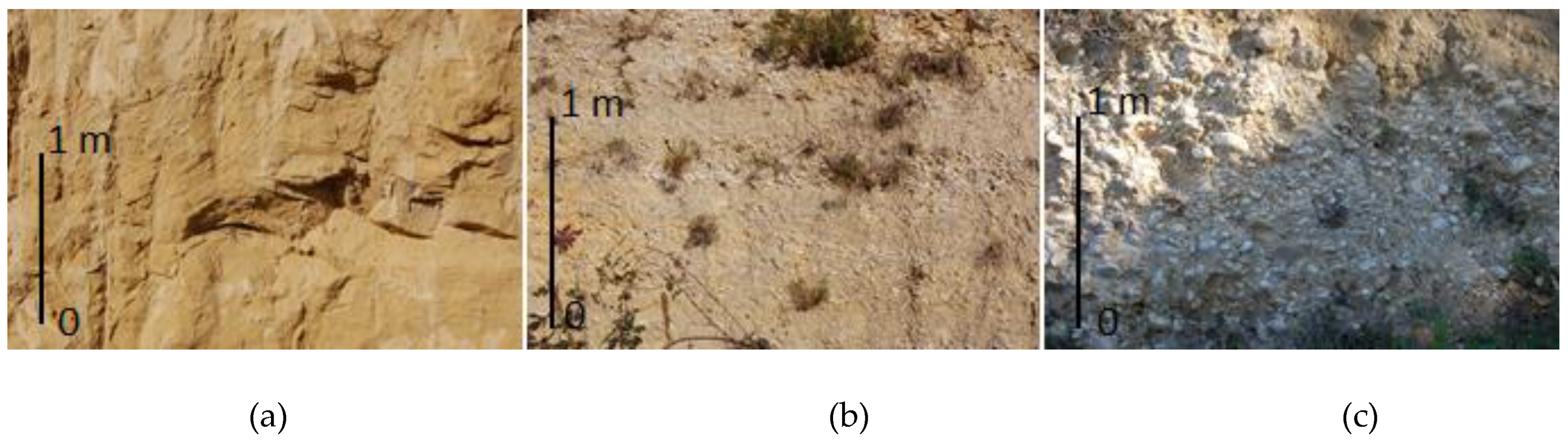
Figure 4.
Some examples of sandy-gravelly association (Arenaceous complex), like they appear in outcrop; (a): mainly arenaceous, (b) arenaceous with gravel, (c) mainly gravelly.
Figure 4.
Some examples of sandy-gravelly association (Arenaceous complex), like they appear in outcrop; (a): mainly arenaceous, (b) arenaceous with gravel, (c) mainly gravelly.
Figure 5.
Geological map and cross-sections of the CH area. (1): Recent alluvial and slope deposits (Holocene); (2): Alluvial deposits (Middle Pleistocene-Holocene); (3): Sandy-gravelly deposits (Middle-Upper Pleistocene); (4): Sandy-clayey deposits (Lower Pleistocene); (5): Marly-clayey deposits (Middle-Upper Pliocene); (6): Sampling well; (7): Pumping test well; (8): Spring; (9): Winter water table contour (m a.s.l.); (10): Cross-section trace; (11): Water table (in cross-section); (12): Spring (in cross-section); (13): Urban area.
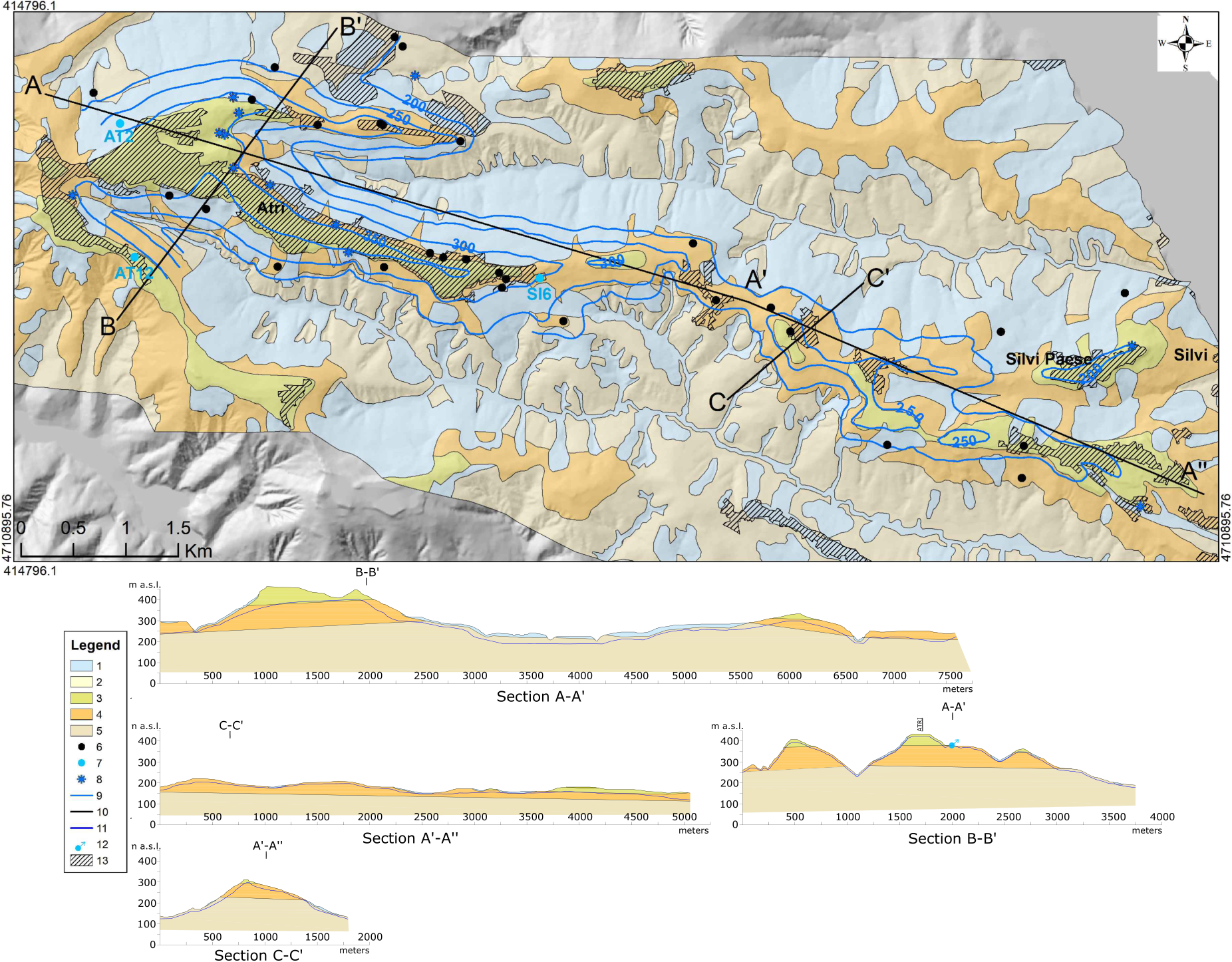
Figure 6.
Geological map and cross-sections of the AS area. (1): Recent alluvial and slope deposits (Holocene); (2): Alluvial deposits (Middle Pleistocene-Holocene); (3): Sandy-gravelly deposits (Middle-Upper Pleistocene); (4): Sandy-clayey deposits (Lower Pleistocene); (5): Marly-clayey deposits (Middle-Upper Pliocene); (6): Sampling well; (7): Pumping test well; (8): Spring; (9): Winter water table contour (m a.s.l.); (10): Cross-section trace; (11): Water table (in cross-section); (12): Spring (in cross-section); (13): Urban area.
Table 1.
Gauging stations (see
Figure 1 for locations).
Table 1.
Gauging stations (see
Figure 1 for locations).
| Area | Observation Period | Gauging Station Name |
|---|
AS
CSA | 1930–2004 | Silvi Alta
Atri |
CH
MA | 1900–2003 | Chieti |
Table 2.
Monitored wells and springs.
Table 2.
Monitored wells and springs.
| Area | Wells | Springs | Monitoring Period |
|---|
| AS | 32 | 12 | 2012–2015 |
| CSA | 21 | 1 | 2014–2015 |
| CH | 88 | 9 | 2005–2015 |
| VI | 36 | 4 | 2007 |
| MA | 22 | 2 | 2012 |
Table 3.
Wintery physico-chemical parameters.
Table 3.
Wintery physico-chemical parameters.
| Winter Period |
|---|
| | | AS | CSA | CH | VI | MA |
|---|
| Temperature (°C) | min | 11 | 7 | 9 | 16 | 11 |
| max | 16 | 16 | 19 | 21 | 15 |
| mean | 13.7 | 14.2 | 14 | 17.9 | 13.9 |
Electric
conductivity
(µS/cm) | min | 259 | 207 | 232 | 346 | 367 |
| max | 1542 | 2130 | 4870 | 939 | 1260 |
| mean | 827.8 | 1127 | 1075 | 646.7 | 602.3 |
| pH | min | 7.1 | 7.4 | 7.3 | | 7 |
| max | 8.7 | 9.2 | 9.2 | | 8.7 |
| mean | 7.9 | 8.1 | 7.9 | | 7.5 |
| Redox potential (mV) | min | 158 | −173 | −140 | | |
| max | 311 | 326 | 225 | | |
| mean | 252 | 225.5 | 153 | | |
Table 4.
Summery physico-chemical parameters.
Table 4.
Summery physico-chemical parameters.
| Summer Period |
|---|
| | | AS | CSA | CH | VI |
|---|
| Temperature (°C) | min | 14 | 15 | 16 | 16 |
| max | 24 | 22 | 25 | 22 |
| mean | 17.7 | 17.5 | 18.6 | 18.9 |
Electric
conductivity
(µS/cm) | min | 179 | 243 | 326 | 349 |
| max | 1410 | 1583 | 4180 | 918 |
| mean | 726 | 1020 | 1076 | 654 |
| pH | min | 6.9 | 7.3 | 7.4 | |
| max | 8.5 | 9.7 | 8.2 | |
| mean | 7.4 | 8 | 7.7 | |
| Redox potential (mV) | min | 27 | −69 | −112 | |
| max | 110 | 281 | 274 | |
| mean | 74.2 | 196 | 166 | |
Table 5.
Water balance from statistical analysis and from the monitoring period.
Table 5.
Water balance from statistical analysis and from the monitoring period.
| Area/Gauging Station | Monitoring Period | Precipitation (mm) | Real Evapotranspiration
(mm) | Potential Evapotranspiration
(mm) | Outflow
(mm) |
|---|
| AS/Silvi Alta | 1930–2004 | 646 | 540 | 808 | 106 |
| AS/Atri | 1930–2004 | 776 | 540 | 765 | 236 |
| CH/Chieti | 1900–2003 | 850 | 579 | 817 | 271 |
| AS/Atri | 2012–2015 | 884 | 609 | 838 | 275 |
| CH/Chieti | 2005–2015 | 800 | 594 | 826 | 206 |
| VI/Chieti | 2007 | 675 | 450 | 851 | 225 |
Table 6.
Yearly specific recharge from historical data.
Table 6.
Yearly specific recharge from historical data.
| Area | Infiltration Area (km2) | Outflow
(mm/y) | Discharge
Coefficient | Infiltration Volume (Mm3/y) | Yearly Specific Recharge (Mm3/y/km2) |
|---|
| AS | 16 | 106 | 0.5 | 0.848 | 0.053 |
| 0.6 | 1.020 | 0.064 |
| CH | 6 | 236 | 0.5 | 0.708 | 0.118 |
| 0.6 | 0.805 | 0.142 |
| VI | 2 | 271 | 0.5 | 0.271 | 0.136 |
| 0.6 | 0.325 | 0.163 |
Table 7.
Yearly specific recharge during monitoring period.
Table 7.
Yearly specific recharge during monitoring period.
| Area | Infiltration Area (km2) | Outflow
(mm/y) | Discharge
Coefficient | Infiltration Volume (Mm3/y) | Yearly Specific Recharge (Mm3/y/km2) |
|---|
| AS | 16 | 275 | 0.5 | 2.200 | 0.138 |
| 0.6 | 2.640 | 0.165 |
| CH | 6 | 206 | 0.5 | 0.621 | 0.104 |
| 0.6 | 0.745 | 0.124 |
| VI | 2 | 225 | 0.5 | 0.202 | 0.101 |
| 0.6 | 0.242 | 0.121 |
Table 8.
Conductivity, transmissivity, and storativity obtained from the pumping test.
Table 8.
Conductivity, transmissivity, and storativity obtained from the pumping test.
| Well | Time
(h) | Saturated Portion Thickness (m) | Method | Conductivity
(K—m/s) | Transmissivity
(T—m2/s) | Storativity
(S) |
|---|
| AT2 | 6 | 2 | 1 | 2.3∙10−4 | 4.7∙10−4 | 16.9 |
| 2 | 1.5∙10−3 | 3.0∙10−3 | |
| 3 | 2.4∙10−4 | 4.8∙10−4 | |
| AT12 | 5 | ~10 | 1 | 8.3∙10−6 | 8.3∙10−5 | 10.3 |
| 2 | 1.8∙10−4 | 1.8∙10−3 | |
| 3 | 7.6∙10−6 | 7.3∙10−5 | |
| SI6 | 6 | 4 | 1 | 4.5∙10−5 | 1.8∙10−4 | 5.1 |
| 2 | 2.2∙10−4 | 9.1∙10−4 | |
| 3 | 3.2∙10−5 | 1.3∙10−4 | |
| CH87 | 4 | ~7 | 1 | 3.1∙10−4 | 2.2∙10−3 | -- |
| 2 | 2.0∙10−5 | 1.4∙10−4 | |
| 3 | 1.3∙10−4 | 9.1∙10−4 | |
Table 9.
Water table fluctuation and yearly specific recharge results.
Table 9.
Water table fluctuation and yearly specific recharge results.
| Area | Infiltration Area
(km2) | Water Table Fluctuation (m) | Effective Porosity (%) | Infiltration Volume
(Mm3) | Water Table Thickness
(mm) | Yearly Specific Recharge (Mm3/y/km2) |
|---|
| AS | 16 | 0.86 | 10 | 1.376 | 86 | 0.086 |
| 15 | 2.064 | 129 | 0.129 |
| CH | 6 | 1.11 | 10 | 0.666 | 111 | 0.111 |
| 15 | 0.990 | 165 | 0.165 |
| VI | 2 | 1.50 | 10 | 0.300 | 166 | 0.150 |
| 15 | 0.450 | 250 | 0.225 |
Table 10.
Estimation of the water resource for three sample sites considering an average saturated thickness in the sandy-gravel association of the arenaceous complex.
Table 10.
Estimation of the water resource for three sample sites considering an average saturated thickness in the sandy-gravel association of the arenaceous complex.
| Area | Infiltration Area
(km2) | Saturated Thickness (m) | Effective Porosity (%) | Total Stored Volume (Mm3) | Infiltration Volume
from Water Level Fluctuation
(Mm3) |
|---|
| AS | 16 | 6 | 10 | 9.600 | 1.376 |
| 15 | 14.300 | 2.064 |
| CH | 6 | 5 | 10 | 3.000 | 0.666 |
| 15 | 4.500 | 0.990 |
| VI | 2 | 4 | 10 | 0.720 | 0.300 |
| 15 | 1.070 | 0.450 |
Table 11.
Yearly specific recharge from total discharge.
Table 11.
Yearly specific recharge from total discharge.
| Area | Period | Spring Water Discharge (L/s) | Spring Water Discharge (Mm3/y) | Infiltration Area (km2) | Infiltration
(mm) | Yearly Specific Recharge (Mm3/y/km2) |
|---|
| AS | Summer | 3.24 | 0.102 | 16 | 6.5 | 0.006 |
| Winter | 6.48 | 0.204 | 16 | 13 | 0.013 |
| Publisher’s Note: MDPI stays neutral with regard to jurisdictional claims in published maps and institutional affiliations. |
© 2021 by the authors. Licensee MDPI, Basel, Switzerland. This article is an open access article distributed under the terms and conditions of the Creative Commons Attribution (CC BY) license (https://creativecommons.org/licenses/by/4.0/).


