Article

Assessment of TOPKAPI-X Applicability for Flood Events Simulation in Two Small Catchments in Saxony

1
Faculty of Environmental Sciences, Department of Hydrosciences, Institute of Urban Water Management, Technical University of Dresden, 01062 Dresden, Germany
2
ON-Oekohydroprojekt, Aiteke bi 120400, Kazakhstan
3
Faculty of Environmental Sciences, Department of Hydrosciences, Institute of Hydrology and Meteorology, Chair of Meteorology, Technical University of Dresden, 01737 Tharandt, Germany
*
Author to whom correspondence should be addressed.
Hydrology 2021, 8(3), 109; https://doi.org/10.3390/hydrology8030109
Submission received: 28 June 2021 / Revised: 21 July 2021 / Accepted: 22 July 2021 / Published: 26 July 2021

Abstract

:
Numerical simulations of rainfall-runoff processes are useful tools for understanding hydrological processes and performing impact assessment studies. The advancements in computer technology and data availability have assisted their rapid development and wide use. This project aims to evaluate the applicability of a physically based, fully distributed rainfall-runoff model TOPKAPI-X for the simulation of flood events in two small watersheds of Saxony, Germany. The results indicate that the model was calibrated well for 4.88 km2 Wernersbach catchment (NSE 0.89), whereas 276 km2 Wesenitz catchment calibration was only satisfactory (NSE 0.7). The addition of the second soil layer improved the model’s performance in comparison to the simulations with only one soil layer for Wernersbach (NSE increase from 0.83 to 0.89). During the validation process, the model showed a variable performance. The best performance was achieved for Wernersbach for the year with the highest runoff (NSE 0.95) in the last decade. The lowest performance for the Wernersbach and Wesenitz catchments was 0.64 for both. The reasons for the model’s low performance in some years are discussed, and include: (i) input data quality and data insufficiency, (ii) methods used within the simulations (interpolation, ETP estimation, etc.), and (iii) assumptions made during the calibration (manual calibration, parameter selection, etc.).

1. Introduction

Floods are one of the most devastating and deadly natural hazards globally, which affect developing and developed countries [1,2]. Germany is not an exception, considering, for example, the flooding events of 2002 in the Elbe River and the Rhine River in 1995 [3]. The most recent example is the floods caused by extreme rainfall in mid-July 2021, which hit the states of Rhineland-Palatinate and North Rhine-Westphalia the worst. In general, this extreme event accounts for one-third of global economic losses and has affected two-thirds of people who have experienced any kind of natural hazard [4]. The authors of [5] have stated that around 50% of water-related disasters worldwide are floods, which affect about 196 million people on a yearly basis in more than 90 states. Due to the natural origin of floods as well as their stochastic nature, complete prevention might not be possible. However, it is possible to lower the related risks and negative consequences by means of real-time flood forecasting systems and the implementation of mitigation actions [2]. In this regard, hydrological models are an essential element in addressing them and in considering potential solutions. As a basis of flood forecasting systems, they simulate the changes in state variables over space and time by representing the internal flow processes [5,6]. The standard procedure for flood forecasting includes the use of numerical watershed hydrological models, which use observed or predicted meteorological variables as boundary conditions, forcing the estimation of discharge [7,8]. In contrast, the simulated runoff would be used as a boundary condition for the hydraulic routing model, which will estimate the flood level and discharge at specific places [2,7]. The primary function of hydrological models is to describe in varying degrees of detail the complex interactions between water, energy, vegetation and simplify this complexity by means of mathematical equations [9,10]. Considering climate change, its influence on the hydrological cycle, and especially its influence on the occurrence of extreme events, modeling is likely to be an essential part of sustainable water resources management in the future [11]. Spatially distributed modeling has become a well-established tool for studying both components of environmental systems and possible changes in them due to their capacity for explicit spatial representation [12]. In order to be able to support the impact assessment studies, such as the influences of climate and land-use change on the hydrological cycle, it is of utmost importance to have models that have a reasonable degree of representation of key physical processes. They should be able to provide the correct answers for the right reasons under the prevailing conditions and, as a result, provide reliable estimates for potential future conditions [9]. It is worth mentioning here that the hydrological cycle is an essential part of environmental systems, as it connects several fields, such as ecology, geology, atmosphere, etc. [9]. More importantly, the combined response of all these fields results in a single output in the form of discharge from the outlet for a given rainfall [9,13]. The situation is complicated by the temporal and spatial variability of all runoff processes, which are determined by the physiographic characteristics of the watershed [14]. Therefore, when hydrological processes are studied, it is essential to use physically appropriate models that are correctly parameterized, calibrated, and evaluated [9].
The digital revolution of the 1960s allowed scientists to simulate the hydrological cycle’s different components and integrate them into a single model [15,16]. Growing computer power, the necessity to better understand natural processes as well as further awareness of the hydrological cycle were the reasons for the enhancement of existing models and for the shift in the development of models from the lumped models to distributed models and from conceptual models to physically based models [17,18,19]. In general, rainfall-runoff models are categorized as lumped or distributed and conceptual, empirical, or physical. In addition, some semi-distributed models assume the distribution of spatial characteristics but avoid the direct modeling of streamflow networks [20]. The authors of [21] reported the inability to represent the spatial heterogeneity, the catchment parameters, and the time-consuming parameter estimation as the main disadvantages of lumped models. To this, the authors of [22] added that it is impossible to solve watershed problems with them, as they rarely represent the observable internal state fluxes. However, the authors of [23] claimed that the power of synthesis makes their use very attractive. According to the authors of [20], semi-distributed models are more advantageous than the fully distributed models due to their simplicity, as the latter tend to over-parameterize and extrapolate small-scale laws to the entire catchment. They also stated that the run time of fully distributed models hinders the assessment of their predictive uncertainty. Even though they are described as giving more plausible results than the lumped models, the parameter identifiability and equifinality problems are a major concern for such models [17,24]. Lower complexity and low driving data requirements were described as the advantages of conceptual distributed and semi-distributed hydrological models. This has resulted in their dominant use for operational practice and catchment scale rainfall-runoff simulations [25,26,27]. Empirical and conceptual models are also characterized by less computational time, making them suitable for real-time applications and Monte Carlo-type scenario simulations (for assessing the predictive uncertainty). However, the parameter identifiability, the need for long historical data for calibration, and their inapplicability for ungauged catchments were reported to be their main disadvantages [24]. There is a consensus in the hydrologic community that physically based, distributed models are powerful tools for representing the real world. They consider spatial information and preserve physical laws (such as the conservation of mass, momentum, and energy) at temporal scales that characterize the underlying physical processes; hence, they are considered better than the lumped and conceptual models [15,26,28,29]. They can explicitly represent and consider the use of assimilation techniques, the observable hydrologic state variables, and fluxes [22]. They also consider the spatio-temporal variability of the main forcings and changes in land-surface properties (for example, soil, vegetation, etc.). The authors of [8,25,30] claimed that they are more suitable for investigating the watershed response to land use and climate change than the empirical and conceptual models. The author of [31] described the direct physical interpretation of model parameters, accuracy, and the capacity for performing comprehensive sensitivity analyses as additional advantages. Thanks to their development which was assisted by the developments in remote sensing, geographic information systems (GIS), and computer technology, they can ensure better results, especially in complex geomorphological and hydrological contexts [18,32,33]. However, they are very data-intensive, time-consuming, and have a complex structure with a large number of parameters [25]. When the model is complex and the basin is large, the major concern is the computational inefficiency, which limits their application for real-time forecasting and Monte Carlo-type scenario simulations [27]. The presence of many parameters is characterized by uncertainty due to the parameter equifinality problem. The problem of equifinality is when several parameter combinations give the best fit, which precludes the choice of the right one [34]. Moreover, the multi-dimensional optimization problem of lumped models becomes hyper-dimensional in distributed models [26]. Another type of model which is used for the simulation of rainfall-runoff models is hydrodynamic models. This approach is sometimes called the direct rainfall method [8,35,36,37,38]. Their application has gained popularity in the last decade due to the improvements in computational power (CPU and GPU) as well as the adoption of different optimization techniques (parallel computing, flow approximation, grid refinement, etc.) [35,36,39,40,41]. Compared to hydrological models that cannot correctly spread the flood dynamics and extents, hydraulic models can reliably predict the highly transient flooding process [2,4].

Background and Rationale of the Current Project

The current study aims to assess the applicability of the hydrological model TOPKAPI-X (TOPographic Kinematic APproximation and Integration-EXtended) to simulate high flow events in two German catchments. The authors of [6,25,42,43] have pointed out the following as the main advantages of the TOPKAPI approach:
(1) Applicability in increasing spatial and temporal scales, while at the same time keeping the physical interpretation of the parameters;
(2) Reduced execution times suitable for distributed model calibrations and real-time operational applications;
(3) Complete use of DEM, soil, as well as land cover maps for obtaining non-linear reservoir cascades and an approximation of model parameters;
(4) Capacity to compute water balance at a highly detailed spatial and temporal resolution by means of combining land use, soil, and other information;
(5) Possibility to track the spatial variability of runoff conditions in the catchment obtaining flow predictions at any point of the channel network;
(6) Physical basis, which allows the linkage between the model parameters and catchment characteristics;
(7) Possibility to run event-based and continuous simulations (climatological studies);
(8) Applicability to ungauged basins due to the possibility of parameter estimation from the literature.
Table 1 demonstrates the comparison of the general characteristics of other hydrological models with TOPKAPI-X.
It is known that the size and shape of the watershed influences the geometry of the enclosed river system, which as a result influences the amount, distribution, and timing of the runoff [70]. In this regard, TOPKAPI-X has been extensively applied for flood forecasting as well as for the estimation of water balance and its components in different watersheds around the world [71]. For example, the authors of [72] have compared TOPKAPI’s (older version of TOPKAPI-X) soil moisture estimate with that of a remotely sensed ASCAT Surface soil moisture product. The results indicated that there is a good correspondence in the dynamic behavior between the results of both sources. In another study, [73] have assessed the sensitivity of TOPKAPI with an added infiltration model (Green-Ampt) to systematic bias in the variables (e.g., rainfall and ETP) as well as in the parameters of the soil component. Overall, the model’s sensitivity was governed by the linear function of the input and the parameter bias. In addition, the sensitivity had the same order of magnitude or a lower order of magnitude than the input and parameter bias. According to the authors of [73], these findings indicate that the model can be robust in relation to errors in forcing and parameters. The authors of [32] applied the modified version to the Upper Xixian catchment and found that it can simulate high and low flow events well. The authors of [74] found that the variable-step fourth-order Runge–Kutta algorithm for the non-linear reservoir equations was a good approximation of subsurface flow in the soil matrix, overland flow over the slopes, and surface flow in the channel network. This allowed the retention of the physical properties of the original equations at scales ranging from a few meters to 1 km. The authors of [23] performed a comparison between the lumped and distributed versions of TOPKAPI. The obtained results showed that it is possible to reproduce the results of the distributed version while at the same time shortening the computation time significantly. However, some limitations were identified on the derivation of the relationship linking the soil water content of the catchment to the extent of the saturated area. The authors of [75] have used TOPKAPI for understanding the response of high-elevation catchments to the changing climate. The authors of [28] simulated the glacier mass balance and demonstrated that the combination of discharge and satellite snow cover could improve the model’s performance. TOPKAPI-ETH, a glacio-hydrological version of the model, has been used to simulate glacier melt and runoff generation in the Nepalese Himalayas [76]. The comparison of TOPKAPI and HEC-HMS for the same catchment showed that TOPKAPI simulates the dynamics of the soil filling, depletion mechanisms, and flood routing in a more unrealistic way [77]. This was assumed to be due to the lack of reservoir modeling in its structure and its hydrograph diffusion effect in the flood wave. The authors of [30] used hourly energy balance simulations together with additional meteorological and surface data to calibrate some of TOPKAPI’s parameters for a glacierized basin in central Chile. They showed that the parameters calibrated in this way responded very clearly to the climate settings typical of the dry Andes of Chile. TOPKAPI-X is used as part of the “Global system for hydrological monitoring and forecasting in real-time at high-resolution GH2MF2” project coupled with the Weather Forecast of Global Circulation Models (Deterministic and Ensembles Run) [78]. It is also being used as part of the real-time flood forecasting system in the Campania region (Southern Italy) as part of the Sele Flood Forecasting System [79].
The current project is different from the previous studies where TOPKAPI has been applied, due to the significantly smaller size of the study areas and the small size of the applied grids (10–40 m here, whereas hundreds of meters to 1 km in other studies). To the authors’ knowledge, TOPKAPI-X has not been applied to German catchments, which is another reason for the assessment of its applicability.

2. Materials and Methods

2.1. Description of the Study Areas

2.1.1. Wernersbach Catchment

The first study site is a small catchment in the Tharandt Forest, in the state of Saxony, Germany (Figure 1a). It has a drainage area of 4.88 km2 and lies in the western part of the forest. Tharandt forest mainly consists of Norway spruce and European beech [80]. Land cover of the Wernersbach catchment consists of Coniferous forest and transitional woodland shrubs, which comprise 94.9 and 5.1% of the area, respectively (Figure 1c). Figure 1 illustrates the locations of the meteorological as well as the hydrological data stations, the Digital Elevation Model (DEM of 10 m resolution), soil type, and land cover maps for this catchment used for modeling.
As the soil map indicates, the main soil type in this catchment is silt (Figure 1c). The bedrock geology is highly variable (gneiss, rhyolite, sandstone, and claystone from the Lower Cretaceous, basalt), forming a mosaic of various soil classes (mostly Dystric Cambisols, Podsols, and Stagnosols). From the geomorphological point of view, the level and gentle-sloped plateaus are predominant, with the height differences between valleys and plateaus ranging between 50 and 100 m [80]. According to the long-term records from the nearby located Grillenburg weather station (1960–2007), the mean annual air temperature is 7.4 °C, whereas the mean annual precipitation is 879 mm [80]. The available hourly discharge data for the Wernersbach Hauptpegel (illustrated in Figure 1a) showed that in the period 2007–2017, the maximum runoff was 6.2 m3/s, the average was 34.93 l/s, while the minimum was 0.19 l/s.

2.1.2. Wesenitz Catchment

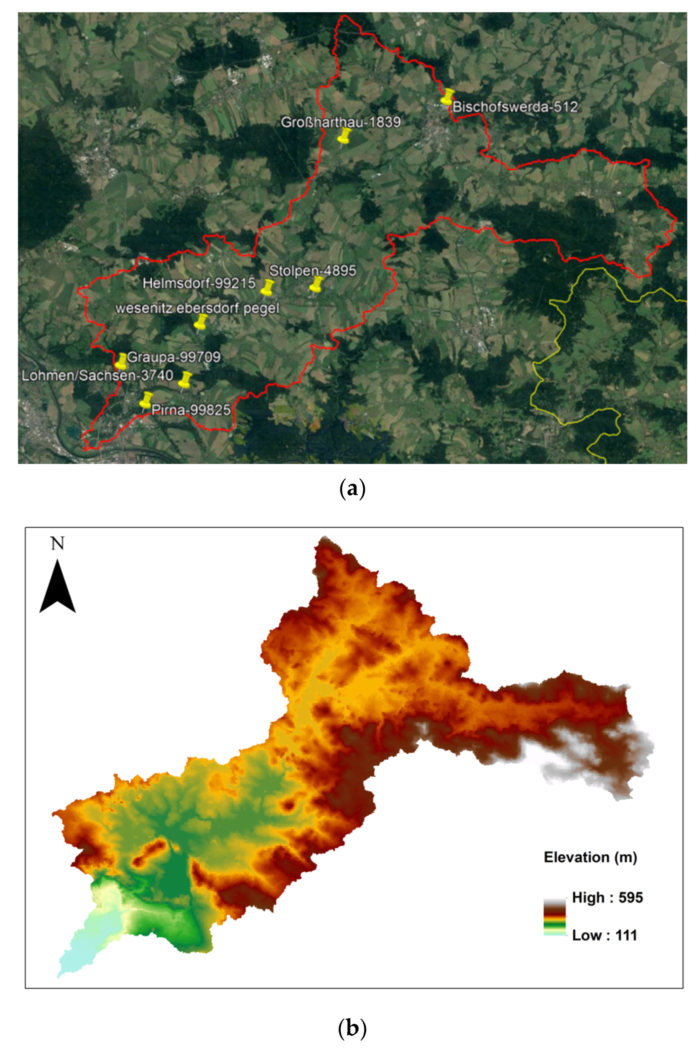
The second study area (Wesenitz) is located in East Saxony (Figure 2a). This river is a right-bank tributary of the Elbe River and originates at the Upper Lusatian Highlands [81]. The contributing catchment area is approximately 276 km2 with a velocity range of 1.5–30 m/s [81,82]. Figure 2 illustrates the DEM of the study area and the locations of rainfall and discharge gauge stations (Wesenitz Elbersdorf Pegel).
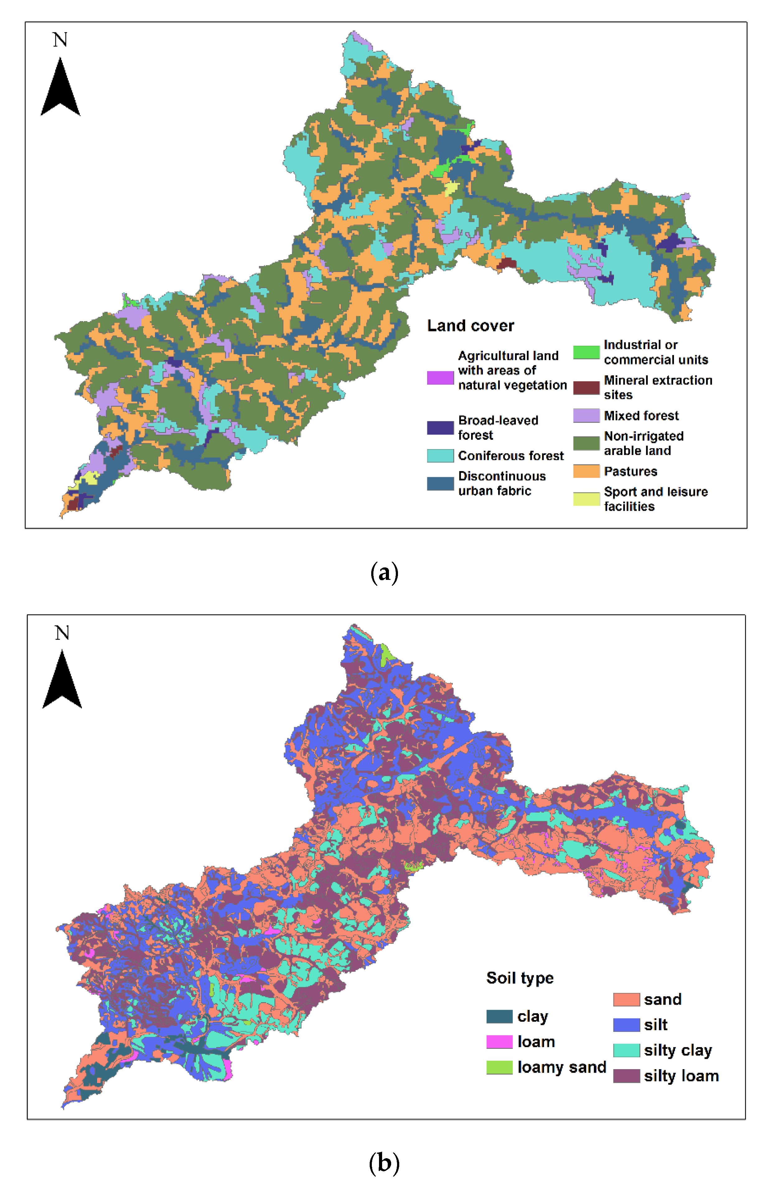
There are 10 land cover and 103 soil classes present in this catchment (Figure 3). This catchment is different from the previous one due to the presence of settlements in its contributing area. As shown in Figure 2, certain parts (eastern side, characterized by a higher elevation) of the catchment were not covered by the rain gauges. The available daily average discharge data for the Elbersdorf gauge indicated that in the period 2005–2015, the maximum flow was 42.6 m3/s, with an average flow of 2.3 m3/s, and a minimum flow of 0.5 m3/s. The land cover map (Figure 3a) shows the dominance of non-irrigated arable land in the catchment. In the soil type map, the major soil type is silt (Figure 3b).

2.2. Description of TOPKAPI-X

TOPKAPI-X (TOPographic Kinematic APproximation and Integration-EXtended) is a fully distributed, physically based rainfall-runoff model [72]. It couples the kinematic wave approach with the topography of the catchment area and transfers the rainfall-runoff as well as the runoff routing processes into three “structurally-similar”, finite dimension, and non-linear reservoir equations [83,84]. Three equations represent (1) drainage in the soil; (2) overland flow on the saturated or impervious soil; and (3) channel flow [18]. The equations are laterally integrated over the grid cells that describe the geometry of the catchment, leading to the cascade of non-linear reservoir equations [42,74]. The channel component is calculated using the kinematic wave method, if the slope is higher than 10−3. When the slope is lower than that value, the Muskingum–Cunge–Todini method is applied for this component [85]. A detailed description of the model is given in [85] and [86]. An overview of the relationships between the equations is well explained by the authors of [43]. To each grid cell, values for physical characteristics are assigned, and in each one of them, the mass and momentum balance computations are performed [83,84]. TOPKAPI-X is a newer version of TOPKAPI. It has several improvements, but the main concepts are those of the original TOPKAPI. The following are the improvements in its formulation [79]:
(1)
Any grid has eight possible flow directions instead of the original four directions;
(2)
The infiltration module is based on the Green-Ampt model, which allows the reproduction of Hortonian processes and accounts for the infiltration excess mechanism;
(3)
The second soil layer is added in order to reproduce different hydrological conditions;
(4)
The addition of the groundwater component based on the cellular automata with full 2D Integrated Finite Difference scheme;
(5)
Introduction of the new coefficients, which consider the sun height with respect to the cell aspect. This is used for the assessment of radiation and albedo in the snow accumulation and melting module based on mass and energy balance;
(6)
The addition of the Reservoir and Lake components.

2.3. Input Data

The Institute of Hydrology and Meteorology of TU Dresden provided the meteorological and hydrological data for both catchments from the relevant sources (Table 2). In the case of Wernersbach, the data was available in hourly time steps, whereas for Wesenitz it was available daily. The temperature data for Wernersbach was obtained from the meteorological station at Grillenburg.
The gaps in the precipitation data for some stations in Wernersbach were filled with the data from the station that had a complete time series. The daily average temperature for Wesenitz was available from only 1 station, and it was taken as a mean for the whole catchment. Due to the absence of data, several ponds (e.g., Niederteich, Waldscheibenteich, etc.) and lakes (such as Natursee, Kiessee, etc.) in this basin were not considered during the simulations. TOPKAPI-X requires several maps in ASCII format as input for pre-processing: filled DEM, basin mask, outlet map, flow direction, flow accumulation, soil, and land cover. Satellite-based DEM (10-m resolution), land Cover, and soil maps for the study areas were provided by the Institute of Hydrology and Meteorology from the corresponding sources (Table 2). All maps were processed in ArcGIS 10.3.1. The model for Wernersbach had a 10-m grid size, whereas the model for Wesenitz had 40-m grids due to model limitations. Table 2 demonstrates the details of the input data used for model generation.

2.4. Model Calibration and Validation

The variability of the parameters within a small range of time and space and uncertainties related to soil characteristics, land cover, etc., necessitated the calibration of the model [18]. Manual calibration was performed for the year with average and variable flows rather than the year with highest flow. As high flow events did not often occur in the considered years, focusing only on them could have biased the calibration. Simulations were performed on hourly time step for Wernersbach (1 October 2009–1 November 2010), while for Wesenitz on daily time step (1 October 2012–1 November 2013). During the calibration, the modeled discharge was visually matched to the recorded flow, while keeping the parameters within their meaningful values and in the same magnitude as in the previous studies with TOPKAPI. The main decisive likelihood function used during the calibration was Nash–Sutcliffe efficiency (NSE). Percentage bias (PBIAS), the coefficient of correlation, and the root mean square error (RMSE) were also calculated and demonstrated in the simulation visualizer tab of TOPKAPI-X. Initial values for all the parameters were derived from the literature. The roughness coefficient for each land cover type was estimated using the values from [1] and they are shown in Table 3 and Table 4. Crop coefficients (Kc) were taken from [87], which are also shown in Table 3 and Table 4.
The calibration of Kc and land cover Manning values was not performed due to the statements in the TOPKAPI-X User Manual about their low sensitivity. The Manning’s value for each Strahler order was taken from [85]. Due to the absence of parameter data on German soil types and the availability of their generic descriptions only, they were simplified to the main soil types (as classified by USDA). Later initial values for these simplified soil types were taken from [85]. As was completed by the authors of [9], shallow soils were assigned to grid cells representing water bodies, rocky areas, and urban areas. All the simulations started in September of the year before the year of interest to allow the warm-up of the model for 1 month and because the snowmelt process required the snow from the previous year. Table 5 and Table 6 show the range of calibrated soil parameters for Wernersbach and Wesenitz, respectively.
Model validation and model calibration are essential prerequisites for the derivation of reliable and accurate discharge estimates from the hydrological models [88]. This should demonstrate the conditions when the model performs well or poorly and confirm that it is acceptable for the intended application [89]. The calibrated model parameters were used for other years (Wernersbach for years 2009, 2012, and 2013, Wesenitz for the years 2006, 2008, and 2010), in order to assess if the model could give reasonably accurate results with another independent datasets. In addition to the above-mentioned goodness of fit (GOF) tests, Mean Error (ME), Mean Absolute Error (MAE), Kling Gupta Efficiency (KGE), Volume Efficiency (VE) and others were applied in order to address the characteristics of the simulated output using the hydroGOF package (developed by Zambrano-Bigiarini) of R-Studio (3.5.1). The equations for the corresponding tests can be found in [90,91,92,93]. For a better visualization and analysis of the results the corresponding plots (such as the scatterplot, the flow duration curve, the hydrograph etc.) were made using the hydroTSM package (developed by Zambrano-Bigiarini) of R-Studio.

3. Results

3.1. Calibration

3.1.1. Wernersbach (One Soil Layer)

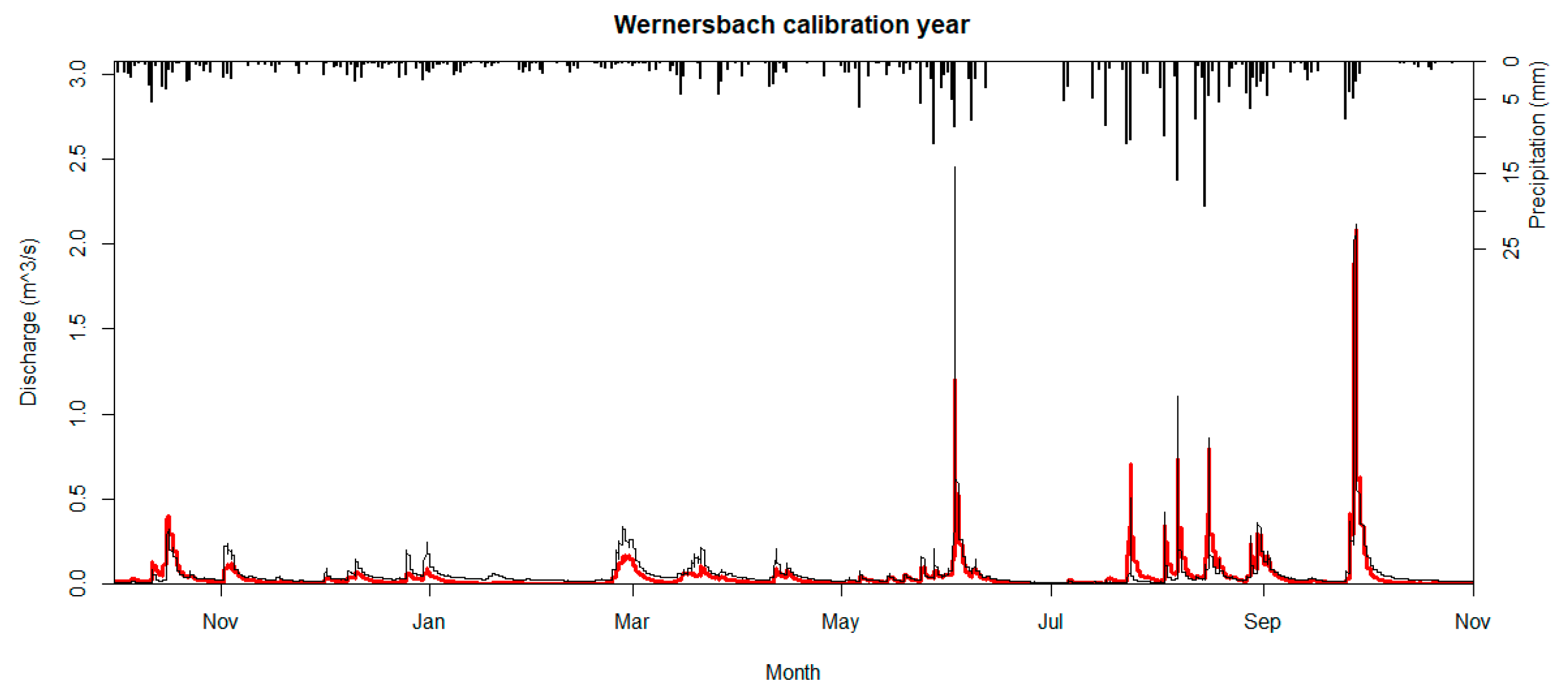
Figure 4 illustrates the simulated and observed runoff hydrograph for the calibration year 2010, when only one soil layer was used (Figure 4). As can be seen, there is a good visual correspondence between the simulated and observed streamflow. In addition to that, the timing of the flow has been well simulated. The NSE test gave 0.83, which is considered good (Table 7) according to the classification by [94]. Though in some cases, the model has underestimated the actual flow.
The peak in June was significantly lower than the observed flow. This underestimation could be due to the assignment of high infiltration capacity for the soil, an incorrect precipitation amount, and the absence of the second soil layer. When there is one soil layer, TOPKAPI-X does not allow the depth of the soil to be more than 50 cm. If the soil is deeper, a second soil layer should be added. The use of a single (shallow) soil layer might have limited the storage capacity of the soil component. The authors of [72] stated that the increase in soil depth could increase the soil saturation index/soil moisture content. Therefore, the shallow soil layer might not act as a significant water holding layer, which otherwise could have led to faster saturation and subsequently a higher runoff generation. As a result, to evaluate the model performance, when the second soil layer was added, the calibration was further performed by the addition of the second soil layer. The developers of TOPKAPI-X have also mentioned the importance of the second soil layer for a better representation of the baseflow (TOPKAPI-X User Manual).

3.1.2. Wernersbach (Two Soil Layers)

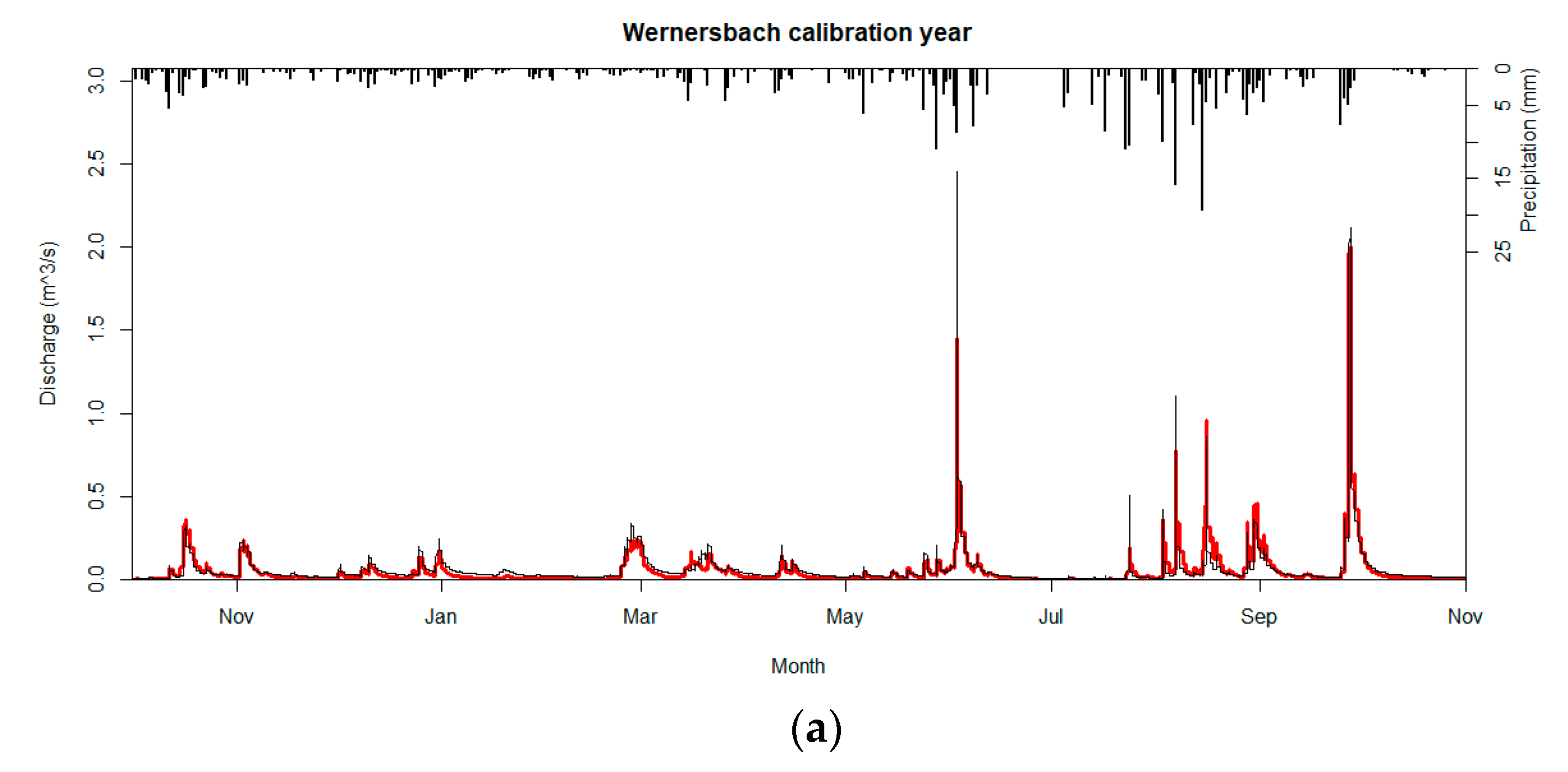
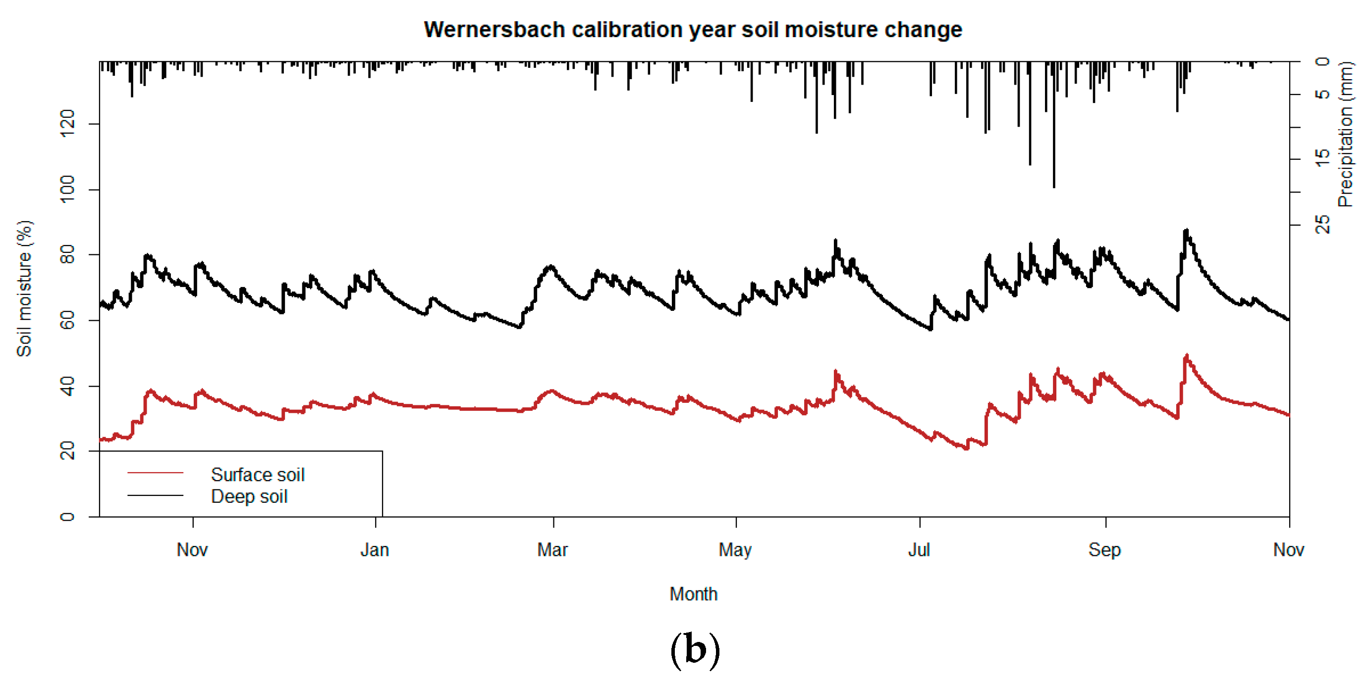
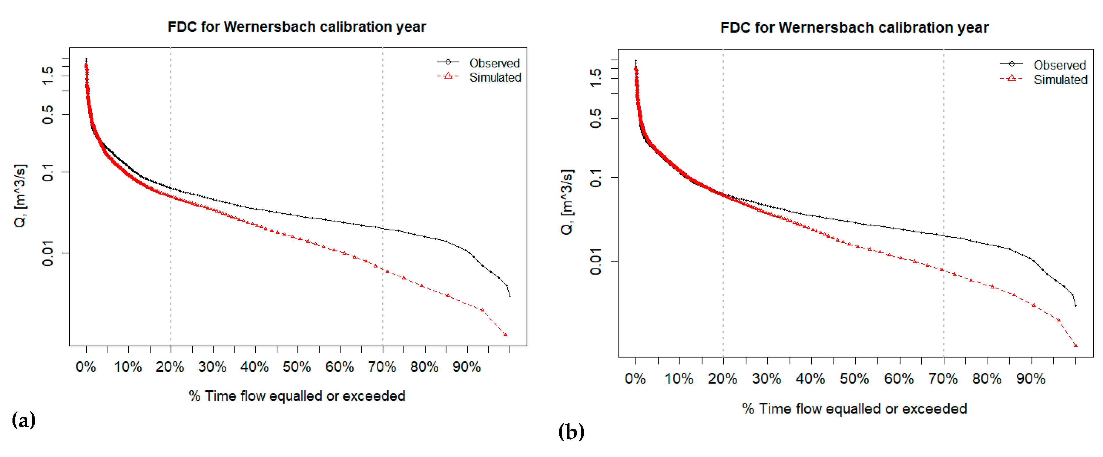
As can be observed from the GOF test results, there was a relatively small improvement (Table 7). The presence of the same underestimation (in June) indicates that the reason for this deviation is not because of the second soil layer absence (Figure 5a). In the original precipitation data, there were gaps during the event in June for the southern rain gauge (located in the highest part of the catchment). As the gaps were filled with the data from another station, this might have resulted in the underrepresentation of the actual rainfall distribution. The presence of significant spatial variability in the precipitation amounts (up to 24 mm) was observed, when the hourly rainfall data from the stations was compared. During the events in June and October, the soil moisture content was of a similar magnitude, though the amount of runoff was not (Figure 5b). This might indicate that the soil was saturated enough, but that the available rain was not enough to result in such a runoff. In the study by the authors of [95] it was found that the runoff generation mechanisms present in the Wernersbach catchment were saturation excess, Hortonian overland flow, and interflow. Due to the lack of data, the Green-Ampt module was not activated, which is responsible for the Hortonian (infiltration excess) overland flow. The authors of [95] claimed that this mechanism was clearly observable during small rain events and was caused by the impermeable roads of 2.6 km length. However, this road was not observable in the available land use map due to the lower resolution of the map. This indicates that modeling with incomplete contributing runoff processes could have caused the observed deviation. The comparison of the flow duration curves (FDC) with one and two soil layers demonstrates which flows were better modeled (Figure 6). Both graphs indicate the poor performance of TOPKAPI-X’s low flow simulation. The authors of [68] explained that the inability of TOPKAPI to simulate the low flows well was due to groundwater module absence. Due to the lack of data, this component was not included, which is likely to have played a role.

3.1.3. Wesenitz

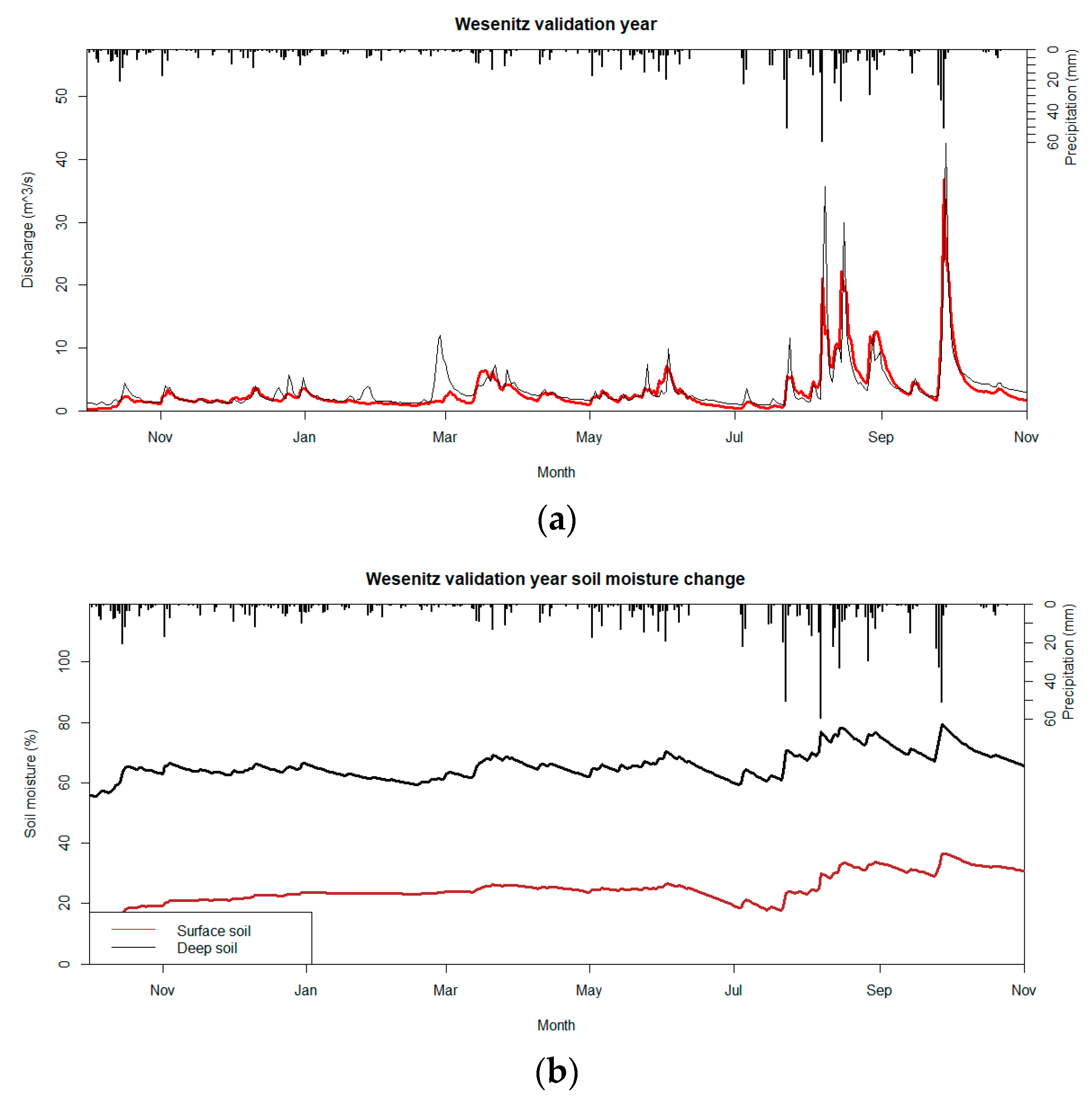
Figure 7 demonstrates the results of the calibration year 2013 for Wesenitz. The results are acceptable (NSE-0.7), but the overall underestimation was relatively high 27.5%. The degree of collinearity between the observed and simulated streamflow data was 60% (Figure 8b). Overall, the model could simulate the time of rises and falls in the hydrograph well, but the problem was with the amount of simulated flow (Figure 7a). Due to a large number of initially estimated parameters resulting from 103 soil classes in this catchment, the global optimum might not have been reached; rather, a local optimum was reached. This could result from manual calibration and its time-consuming nature, as a result of which it is not possible to consider the whole parameter space and all the possible combinations. Considering the improvement in the model’s performance in the case of the Wernersbach catchment, the calibration for Wesenitz started with two soil layers from the beginning. The soil moisture graph does not show a high variability, probably due to the daily averaging of the data (Figure 7b).
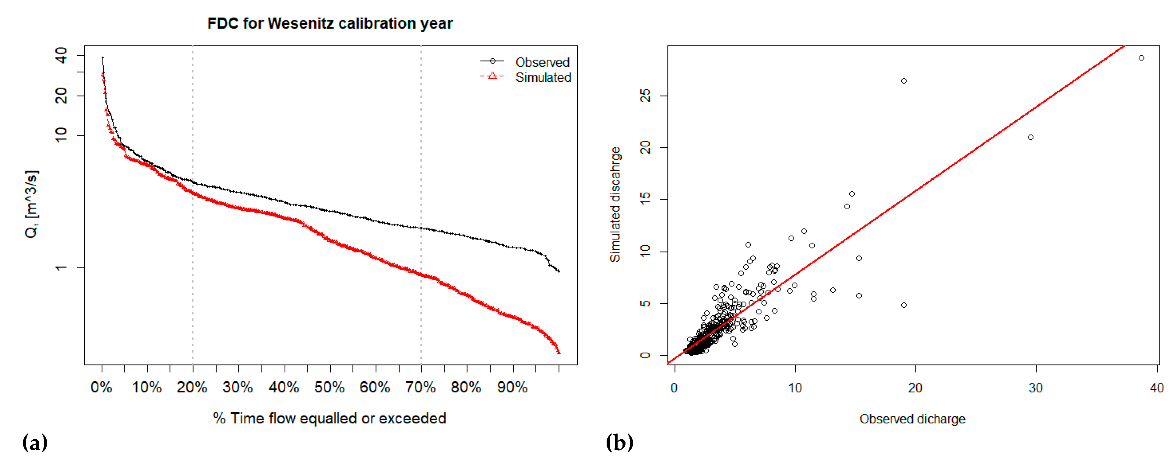
The FDC and scatterplot show that the model underrepresented the low flows significantly, which could also be due to the fact the groundwater component was not included (Figure 8). FDC demonstrates that the model struggled to simulate low flows, as the discrepancy between the simulated and observed flow increased with a decrease in the flow volume (Figure 8a). The authors of [96] claimed that calibration with NSE concentrates more on the high flows of the hydrograph at the expense of improvements to the low flow predictions. In addition, the authors of [97] stated that certain problems could arise as a result of bias normalization and the tendency for the systematic underestimation of flow variability. They found that optimization using NSE can lead to the underestimation of variability in the calibration period, which will later propagate to the validation period. As a result, at certain cases the low flows would be poorly represented after calibration with NSE.

3.2. Validation Period

3.2.1. Wernersbach

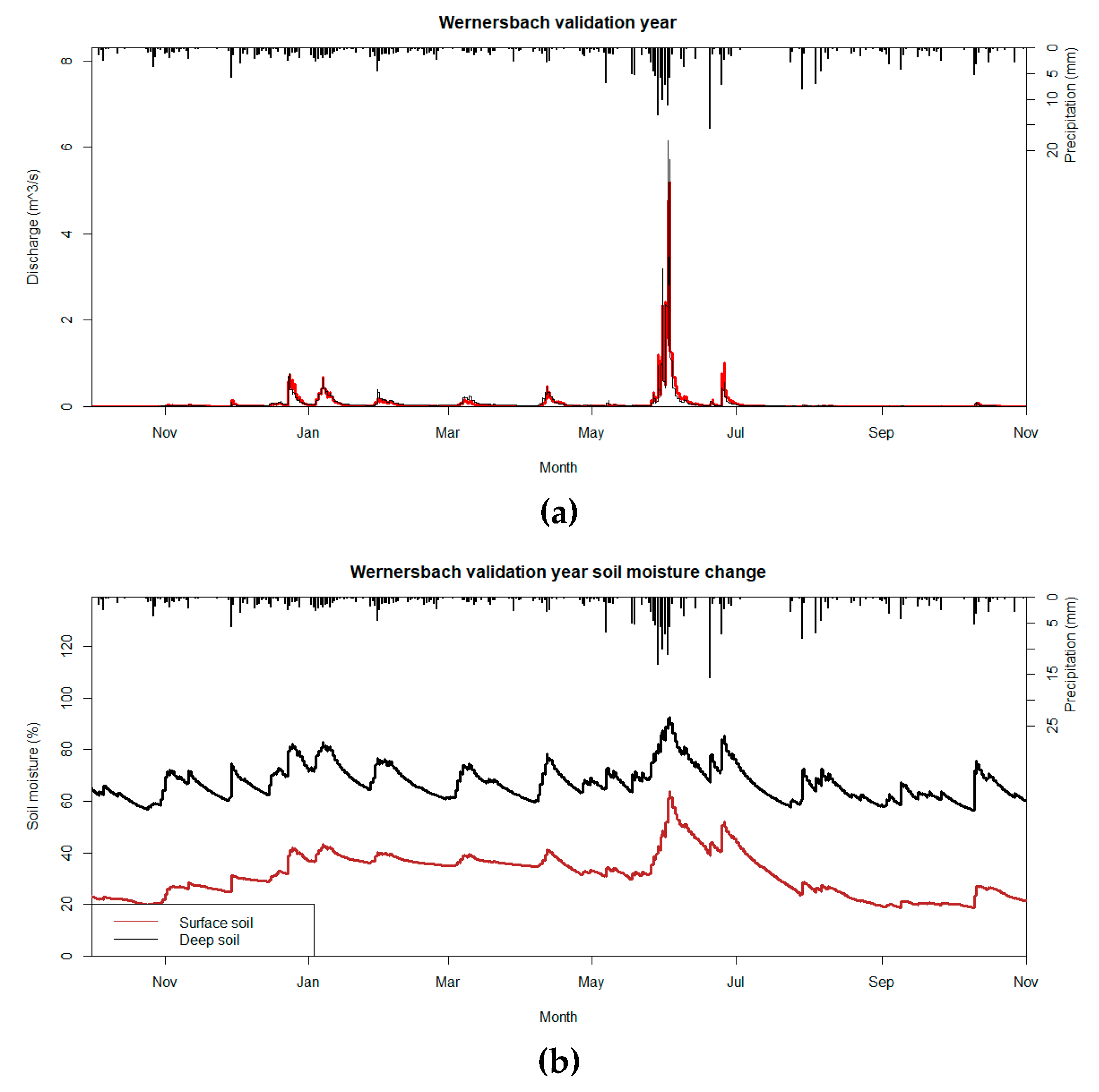
The validation of the model with the year with the recent high flow event is described next. The year with the highest flow in the last decade gave the best fit in the case of the Wernersbach catchment in comparison to the other validation years (Table 8). There was overall a good fit between the simulated and observed runoff time series (Figure 9a).
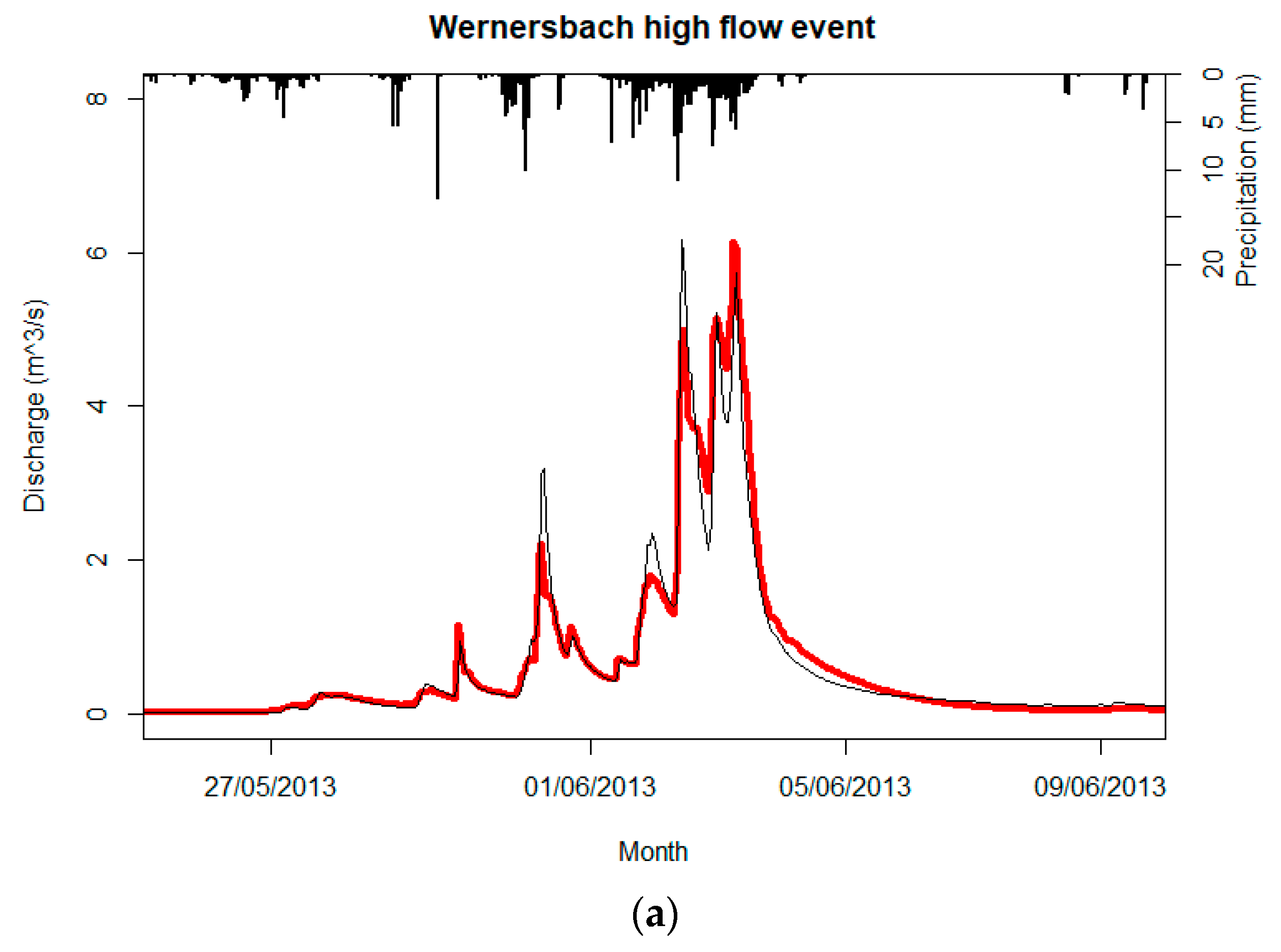
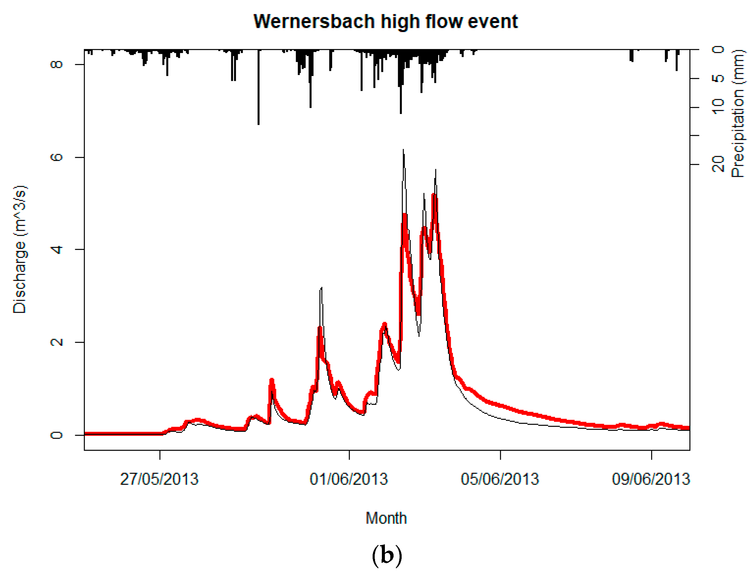
As can be seen from the soil moisture map, the significant runoff is noticeable when the soil moisture goes above 80% (Figure 9b). Even though the overall fit is very good (NSE-0.95) and the overall underestimation percentage is low (PBIAS-1.4%), the highest flow has been significantly underestimated with a relative error value of 25.6% (Figure 10a,b). Among all the GOF tests, only the volume efficiency coefficient showed a significant difference between the simulated and observed values (VE-0.69). Among three validation years, the model’s performance was lowest for the year 2012 (NSE-0.64). This year also had the highest underestimation (−14.2), but the lowest RMSE and MAE values. For the year 2009 the model performance was acceptable (NSE-0.71) and the underestimation was within the accepted limits (−6.9). The main difference between the year 2013 and the other two validation years is the fact that in the latter there was no high flow. So, the calibrated model showed very good results for a high flow event, whereas for average years the model’s performance degraded.
In order to have a better look at this peak flow event, a closer view is provided in Figure 10, when one and two soil layers were used. The model represents well the rising and falling limbs. However, the highest flow has been underestimated in both cases. The case with two soil layers underestimated all the peaks during this event, whereas the case with one soil layer overestimated the second part of the event. To put it another way, two soil layers are not saturated enough, whereas one soil layer is saturating faster and generating a higher runoff during this event.

3.2.2. Wesenitz

The model’s performance had degraded when the model was validated for Wesenitz with the year 2010. A visual analysis showed that the model represented the patterns of the hydrograph well, though the coefficient of the determination test gave only 0.55 (Figure 11a, Table 8). The relative error between the observed highest flow and the simulated highest flow was around −13.6%. The model performance in terms of the NSE coefficient was the lowest among the validated years (0.64), whereas the KGE coefficient was the highest (0.79) (Table 8). The overall underestimation was less than 10%, which is acceptable. It should be pointed out that analyzing the model performance with only 365 points might not be statistically valid and significant. The small peak at the end of February is probably due to the snow melting process. However, the model calculated a significantly lower flow. Considering that this peak did not occur later in the spring, it could be hypothesized that the model was not provided with sufficient snow. This could be due to the lower coverage of the catchment with the precipitation gauges, as the available gauges might have underrepresented the available snow. The soil moisture graph shows that the deeper layer was mostly stable from January to June (Figure 11b). In general, the results for this catchment are acceptable, although further research should be completed with hourly data and with a better rain gauge coverage of the area. Considering the large number of parameters, the problems mentioned earlier (i.e., local optimum, equifinality problem) cannot be excluded in this modeling setup. The two other years used for validation (2006 and 2008) showed better performances than the year with highest flow (NSE 0.72 and 0.67, respectively). Interestingly, in the case of Wesenitz, the model performance during validation did not show significant variation among the years (0.64–0.72), as was observed for Wernersbach. The year 2006 demonstrated the best model performance in terms of NSE, however its overall underestimation was also highest. The volumetric efficiency values were also in close range.

4. Discussion

The importance and usefulness of hydrological models for water resources management, for understanding the hydrological processes and for impact assessment studies is clear. They are important tools which allow scientists as well as policy-makers to make decisions based on the simulations of catchment behavior [9]. Considering the increasing demand for water and the influence of climate change, they will clearly be part of future water management practices. The current study results illustrated that TOPKAPI-X has the potential to simulate the runoff at small catchments of Saxony. According to the authors of [12], the model performance can vary depending on many factors, such as the model structure, the physiographic characteristics of the basin, and the available data (resolution, accuracy, and quantity). Their main point was that no single model is perfect and best for all problems. Similarly, the findings of this study showed that different conditions result in varying representations of the rainfall-runoff processes at each watershed. On the one hand (e.g., Wernersbach) the model gave very good results; on the other hand (Wesenitz), the results were only satisfactory. An analysis of the results and the available literature has shown that there are several potential sources of error, which will be discussed next.

4.1. Sources of Error

4.1.1. Missing Data and the Lack of Precipitation Data

In general, the quality and availability of the precipitation data are essential for hydrologic analysis and the design of water resources systems [98]. Nevertheless, the availability of complete data is not common. However, the authors of [99] pointed out that the precipitation variability has a significant influence on the peak flows at small scales. In the case of the Wernersbach catchment, there were gaps in the precipitation data for certain stations. The filling of these gaps might have added bias to the spatial distribution of precipitation. This was a necessary step as the cumulative difference in the precipitation was significant and not filling them would have resulted in even higher errors. The authors of [9] stated that the presence of elevation variation in an order of more than 100 m could result in the pronounced temporal and spatial variations of the climatic elements. Both catchments had these characteristics, which could mean that the existing rain gauge density might not be enough to exhibit the prevailing meteorological conditions in the catchment. Consequently, this would lead to a pronounced over or underestimation of the rainfall amount. In addition to the above-mentioned points, it is worth mentioning that the hydrological data are subject to significant uncertainty and error (systematic and random) [33,98]. They are described to be critical, as they can affect the continuity of rainfall data and ultimately influence the results of the hydrologic models, which rely heavily on them [100].

4.1.2. Spatial Distribution of Precipitation (Interpolation Method)

The outcomes of hydrological models rely on the space–time structure of atmospheric inputs, which is usually provided by interpolation methods [101,102]. Regarding this, the authors of [102,103] reported that the spatial variability of precipitation especially at fine scales significantly impacts the catchment response, the estimation of model parameters, and the volume and the timing of the peak flow. The errors in the areal extent or in the amount of precipitation will directly lead to large errors in the simulated flow and to the compensation for the input errors by wrong parameter adjustment [101,102]. TOPKAPI-X uses the Thiessen Polygon method for the interpolation of the rainfall. It is a well-known, simple technique for estimating mean areal rainfall based on proximal mapping [98,104]. It might pose limitations to the adequate representation of precipitation distribution. This problem is especially important in the case of sparsely distributed rain gauges, as the authors of [101] stated that this might result in an over or underestimation of the total rainfall amount. The authors of [104] stated the following as its disadvantages: (1) unsuitability for mountainous and hilly regions; (2) unrealistic patchy maps with sudden changes at the polygon boundaries; and (3) loss of information on rainfall gradients. It is possible to input precipitation data distributed by other techniques (e.g., Kriging, inverse distance weighting, etc.) by means of prepared precipitation maps. However, this option was not considered in the current project.

4.1.3. Lack of Information on Parameters and Resulting Uncertainties

The basis of physically based models is that the parameters can be measured and used by tuning during calibration [75]. However, the authors of [105] stated that the measurement of model parameters is not possible due to the presence of preferential flows. In this project, there was no data available regarding the parameters for these specific locations; as a result, they had to be estimated. The approximation of all the parameters can lead to increased uncertainties in the model performance and output errors. As the authors of [106] stated, the uncertainties during calibration would consequently propagate to the model output. The situation becomes more complicated as some properties can significantly vary even in a relatively homogeneous area (e.g., soil hydraulic properties and water content) [63,80]. On top of this, the strong interaction between the parameters further complicates the situation [89]. The authors of [5] pointed out that the use of land cover-defined Manning’s coefficients is acceptable in medium and large catchments, whereas in small catchments (or at subcatchment level) their use can introduce significant errors to the results.

4.1.4. Manual Calibration with One Aggregated Response

The process of calibration faces several challenges related to the nature of hydrological models, such as nonlinearity, data errors and insufficiency, correlation among parameters, irregular response surfaces, and the single or multi-objective nature of the models [107]. As mentioned earlier, the manual calibration performed in this study could not consider the problem of equifinality and the whole parameter space. The authors of [9,100] stated that manual calibration is time-consuming, partially subjective, and only feasible when a trained and experienced user performs it. However, the authors of [89] mentioned the limited repeatability, the difficulty for the cases with more than ten parameters, and the amenability for the calibration of one gauge at a time as the major drawbacks of this method. Moreover, when manual calibration is used, it is hard to identify when the best fit has been obtained [100]. Another important point is the uncertainties related to the use of a single integrated response (e.g., discharge). The authors of [30,75] stated that the use of a single integrated response might result in the problem of equifinality. In addition, this does not guarantee the correct reproduction of single internal processes and cannot avoid the compensation of the errors by the different model components [30]. Therefore, in the case of the physically based, distributed models, model calibration should include the use of spatially distributed observations to avoid the parameter identifiability problem, producing a better balance between modeled processes and a better partitioning of the variable runoff components [108].

4.1.5. Insufficient or Inaccurate Processes

Due to the lack of data, several components and modules were not activated during the simulations, such as the Lakes and Reservoir component (for Wesenitz), the Green-Ampt Module, and the Groundwater component (for both watersheds). Their activation could have improved the model performance. In addition, interception might not have been adequately considered in TOPKAPI-X. The author of [109] stated that neglecting interception could introduce significant errors, which would propagate into the subsequent processes simulated (such as soil moisture and groundwater recharge). The authors of [17] found that including an interception in the simulation improved the stream flow modeling due to better soil moisture accounting. The authors of [110] added that the influence of interception losses is noticeable only during small storms and only influences the surface runoff rate. Evapotranspiration (ETP) directly influences the runoff, soil water storage, local precipitation, and temperature at the regional scale [110]. The authors of [56] mentioned that the correct estimation of ETP is essential for obtaining the correct total discharge volume. The use of a simplistic method by TOPKAPI-X might be another reason for the low model performance at certain years. According to the authors of [110], the crop coefficient method works well for irrigation agriculture, where uniform phenology is present. In the case of forests, it is considered problematic due to the large variability of species composition, leaf biomass dynamics throughout the season, age, and the density effects on tree biomass and water transport properties.

5. Conclusions

The use of the rainfall-runoff models for the management of water resources and for the simulation of historical events is associated with many benefits. With the proper calibration using a variety of historical events, the model could be used for impact assessment studies and the simulation of future events. The current project aimed to assess the applicability of TOPKAPI-X for the simulation of historical flood events in small scale German watersheds using high spatial resolution maps. The study areas had different sizes and varying land cover and soil types. In general, TOPKAPI-X demonstrated a relatively good performance for the chosen study areas. For the Wernersbach catchment, the obtained results were good (NSE 0.83-0.95), though certain events were significantly underestimated. In comparison to the simulations with only one soil layer, the addition of the second soil layer improved the model’s performance. The simulations of the Wesenitz catchment were only acceptable (NSE 0.64-0.72), as in some years, the degree of underestimation was high. In this case, the lack of data for certain parts of the catchment might have resulted in a low NSE coefficient. The manual calibration of a large number of parameters might not have guaranteed the best fit. The literature review, the analysis of the input data, as well as the model structure indicated that there could be several sources of error, such as: (1) missing and insufficient precipitation data; (2) the interpolation method used; (3) lack of information on parameters; (4) manual calibration using a single integrated response; and (5) insufficient and inaccurate processes inclusion. It is expected that accounting for and considering the above-mentioned error sources will significantly improve the model’s performance.

Author Contributions

Conceptualization, N.O. and F.A.J.; methodology, F.A.J. and N.O.; software, N.O.; validation, N.O. and F.A.J.; formal analysis, N.O.; investigation, F.A.J.; resources, F.A.J.; data curation, N.O., F.A.J., J.D.R.S. and J.B.; writing—original draft preparation, N.O.; writing—review and editing, N.O., F.A.J., C.B. and P.K.; visualization, N.O.; supervision, F.A.J., P.K. and C.B.; project administration, F.A.J.; funding acquisition, C.B. All authors have read and agreed to the published version of the manuscript.

Funding

Open Access Funding by the Publication Fund of the TU Dresden.

Data Availability Statement

Not applicable.

Conflicts of Interest

The authors declare no conflict of interest. The funders had no role in the design of the study; in the collection, analyses, or interpretation of data; in the writing of the manuscript, or in the decision to publish the results.

References

  1. Pestana, R.; Matias, M.; Canelas, R.; Araújo, A.; Roque, D.; Van Zeller, E.; Trigo-Teixeira, A.; Ferreira, R.; Oliveira, R.; Heleno, S. Calibration of 2D Hydraulic Inundation models in the Floodplain Region of the Lower Tagus River. In Proceedings of the ESA Living Planet Symposium, Edimburgh, UK, 9–13 September 2013. [Google Scholar]
  2. Ming, X.; Liang, Q.; Xia, X.; Li, D.; Fowler, H.J. Real-Time Flood Forecasting Based on a High-Performance 2-D Hydrodynamic Model and Numerical Weather Predictions. Water Resour. Res. 2020, 56, e2019WR025583. [Google Scholar] [CrossRef]
  3. Werner, M.; Reggiani, P.; Roo, A.D.; Bates, P.; Sprokkereef, E. Flood Forecasting and Warning at the River Basin and at the European Scale. Nat. Hazards 2005, 36, 25–42. [Google Scholar] [CrossRef]
  4. Xia, X.; Liang, Q.; Ming, X. A Full-Scale Fluvial Flood Modelling Framework Based on a High-Performance Integrated Hydrodynamic Modelling System (HiPIMS). Adv. Water Resour. 2019, 132, 103392. [Google Scholar] [CrossRef]
  5. Kalyanapu, A.J.; Burian, S.J.; McPherson, T.N. Effect of land use-based surface roughness on hydrologic model output. J. Spat. Hydrol. 2009, 9, 51–71. [Google Scholar]
  6. Soderman, D.; Meneguzzo, F.; Gozzini, B.; Grifoni, D.; Messeri, G.; Rossi, M.; Montagnani, S.; Pasqui, M.; Orlandi, A.; Ortolani, A.; et al. Very High Resolution Precipitation Forecasting on Low Cost High Performance Computer Systems in Support of Hydrological Modeling. In Proceedings of the 17th Conference on Hydrology, AMS Annual Meeting, Long Beach, CA, USA, 9–13 February 2003. [Google Scholar]
  7. De Roo, A.P.J.; Gouweleeuw, B.; Thielen, J.; Bartholmes, J.; Bongioannini-Cerlini, P.; Todini, E.; Bates, P.D.; Horritt, M.; Hunter, N.; Beven, K.; et al. Development of a European Flood Forecasting System. Int. J. River Basin Manag. 2003, 1, 49–59. [Google Scholar] [CrossRef]
  8. Caviedes-Voullième, D.; Fernández-Pato, J.; Hinz, C. Performance Assessment of 2D Zero-Inertia and Shallow Water Models for Simulating Rainfall-Runoff Processes. J. Hydrol. 2020, 584, 124663. [Google Scholar] [CrossRef]
  9. Viviroli, D.; Zappa, M.; Gurtz, J.; Weingartner, R. An introduction to the hydrological modelling system PREVAH and its pre- and post-processing-tools. Environ. Model. Softw. 2009, 24, 1209–1222. [Google Scholar] [CrossRef]
  10. Zhao, L.; Xia, J.; Xu, C.; Wang, Z.; Sobkowiak, L.; Long, C. Evapotranspiration estimation methods in hydrological models. J. Geogr. Sci. 2013, 23, 359–369. [Google Scholar] [CrossRef]
  11. Te Linde, A.H.; Aerts, J.C.J.H.; Hurkmans, R.T.W.L.; Eberle, M. Comparing model performance of two rainfall-runoff models in the Rhine basin using different atmospheric forcing data sets. Hydrol. Earth Syst. Sci. Discuss. 2007, 4, 4325–4360. [Google Scholar]
  12. Liu, J.; Chen, X.; Zhang, J.; Flury, M. Coupling the Xinanjiang model to a kinematic flow model based on digital drainage networks for flood forecasting. Hydrol. Process. 2009, 23, 1337–1348. [Google Scholar] [CrossRef]
  13. Koch, J.; Cornelissen, T.; Fang, Z.; Bogena, H.; Diekkrüger, B.; Kollet, S.; Stisen, S. Inter-Comparison of Three Distributed Hydrological Models with Respect to Seasonal Variability of Soil Moisture Patterns at a Small Forested Catchment. J. Hydrol. 2016, 533, 234–249. [Google Scholar] [CrossRef]
  14. Uhlenbrook, S. An Empirical Approach for Delineating Spatial Units with the Same Dominating Runoff Generation Processes. Phys. Chem. Earth Parts A/B/C 2003, 28, 297–303. [Google Scholar] [CrossRef]
  15. Todini, E. Hydrological catchment modelling: Past, present and future. Hydrol. Earth Syst. Sci. Discuss. 2007, 11, 468–482. [Google Scholar] [CrossRef] [Green Version]
  16. Chiew, F.H.S. Lumped Conceptual Rainfall-Runoff Models and Simple Water Balance Methods: Overview and Applications in Ungauged and Data Limited Regions. Geogr. Compass 2010, 4, 206–225. [Google Scholar] [CrossRef]
  17. Zhang, G.P.; Savenije, H.H.G. Rainfall-runoff modelling in a catchment with a complex groundwater flow system: Application of the Representative Elementary Watershed (REW) approach. Hydrol. Earth Syst. Sci. Discuss. 2005, 9, 243–261. [Google Scholar] [CrossRef] [Green Version]
  18. Yan, Y.; Tao, X.; Li, B.; Mazzetti, C. Application of hydrometeorological coupled European flood forecasting operational real time system in Yellow River Basin. Water Sci. Eng. 2009, 2, 28–39. [Google Scholar] [CrossRef]
  19. Paiva, R.C.D.; Collischonn, W.; Tucci, C.E.M. Large scale hydrologic and hydrodynamic modeling using limited data and a GIS based approach. J. Hydrol. 2011, 406, 170–181. [Google Scholar] [CrossRef]
  20. Kavetski, D.; Kuczera, G.; Franks, S.W. Semidistributed Hydrological Modeling: A “Saturation Path” Perspective on TOPMODEL and VIC. Water Resour. Res. 2003, 39. [Google Scholar] [CrossRef] [Green Version]
  21. Storck, P.; Bowling, L.; Wetherbee, P.; Lettenmaier, D. Application of a GIS-Based Distributed Hydrology Model for Prediction of Forest Harvest Effects on Peak Stream Flow in the Pacific Northwest. Hydrol. Process. 1998, 12, 889–904. [Google Scholar] [CrossRef]
  22. Fatichi, S.; Vivoni, E.R.; Ogden, F.L.; Ivanov, V.Y.; Mirus, B.; Gochis, D.; Downer, C.W.; Camporese, M.; Davison, J.H.; Ebel, B.; et al. An Overview of Current Applications, Challenges, and Future Trends in Distributed Process-Based Models in Hydrology. J. Hydrol. 2016, 537, 45–60. [Google Scholar] [CrossRef] [Green Version]
  23. Martina, M.L.V.; Todini, E.; Liu, Z. Preserving the dominant physical processes in a lumped hydrological model. J. Hydrol. 2011, 399, 121–131. [Google Scholar] [CrossRef]
  24. Hapuarachchi, H.A.P.; Wang, Q.J.; Pagano, T.C. A Review of Advances in Flash Flood Forecasting. Hydrol. Process. 2011, 25, 2771–2784. [Google Scholar] [CrossRef]
  25. Zhao, G.; Hörmann, G.; Fohrer, N.; Gao, J.; Li, H.; Tian, P. Application of a Simple Raster-Based Hydrological Model for Streamflow Prediction in a Humid Catchment with Polder Systems. Water Resour. Manag. 2011, 25, 661–676. [Google Scholar] [CrossRef]
  26. Khakbaz, B.; Imam, B.; Hsu, K.; Sorooshian, S. From lumped to distributed via semi-distributed: Calibration strategies for semi-distributed hydrologic models. J. Hydrol. 2012, 418–419, 61–77. [Google Scholar] [CrossRef] [Green Version]
  27. Sayama, T.; Tachikawa, Y.; Takara, K. Spatial lumping of a distributed rainfall-sediment-runoff model and its effective lumping scale. Hydrol. Process. 2012, 26, 855–871. [Google Scholar] [CrossRef]
  28. Finger, D.; Pellicciotti, F.; Konz, M.; Rimkus, S.; Burlando, P. The value of glacier mass balance, satellite snow cover images, and hourly discharge for improving the performance of a physically based distributed hydrological model. Water Resour. Res. 2011, 47. [Google Scholar] [CrossRef]
  29. Aureli, F.; Prost, F.; Vacondio, R.; Dazzi, S.; Ferrari, A. A GPU-Accelerated Shallow-Water Scheme for Surface Runoff Simulations. Water 2020, 12, 637. [Google Scholar] [CrossRef] [Green Version]
  30. Ragettli, S.; Pellicciotti, F. Calibration of a physically based, spatially distributed hydrological model in a glacierized basin: On the use of knowledge from glaciometeorological processes to constrain model parameters. Water Resour. Res. 2012, 48. [Google Scholar] [CrossRef]
  31. Elsafi, S.H. Artificial Neural Networks (ANNs) for flood forecasting at Dongola Station in the River Nile, Sudan. Alex. Eng. J. 2014, 53, 655–662. [Google Scholar] [CrossRef]
  32. Liu, Z.; Martina, M.L.V.; Todini, E. Flood forecasting using a fully distributed model: Application of the TOPKAPI model to the Upper Xixian Catchment. Hydrol. Earth Syst. Sci. Discuss. 2005, 9, 347–364. [Google Scholar] [CrossRef] [Green Version]
  33. McMillan, H.K.; Booker, D.J.; Cattoën, C. Validation of a national hydrological model. J. Hydrol. 2016, 541, 800–815. [Google Scholar] [CrossRef]
  34. Grayson, R.B.; Blöschl, G.; Western, A.W.; McMahon, T.A. Advances in the use of observed spatial patterns of catchment hydrological response. Adv. Water Resour. 2002, 25, 1313–1334. [Google Scholar] [CrossRef]
  35. Costabile, P.; Costanzo, C.; Ferraro, D.; Macchione, F.; Petaccia, G. Performances of the New HEC-RAS Version 5 for 2-D Hydrodynamic-Based Rainfall-Runoff Simulations at Basin Scale: Comparison with a State-of-the Art Model. Water 2020, 12, 2326. [Google Scholar] [CrossRef]
  36. Ferraro, D.; Costabile, P.; Costanzo, C.; Petaccia, G.; Macchione, F. A Spectral Analysis Approach for the a Priori Generation of Computational Grids in the 2-D Hydrodynamic-Based Runoff Simulations at a Basin Scale. J. Hydrol. 2020, 582, 124508. [Google Scholar] [CrossRef]
  37. Fernández-Pato, J.; Martínez-Aranda, S.; García-Navarro, P. A 2D Finite Volume Simulation Tool to Enable the Assessment of Combined Hydrological and Morphodynamical Processes in Mountain Catchments. Adv. Water Resour. 2020, 141, 103617. [Google Scholar] [CrossRef]
  38. Ni, Y.; Cao, Z.; Liu, Q.; Liu, Q. A 2D Hydrodynamic Model for Shallow Water Flows with Significant Infiltration Losses. Hydrol. Process. 2020, 34, 2263–2280. [Google Scholar] [CrossRef]
  39. Cea, L.; Bladé, E. A Simple and Efficient Unstructured Finite Volume Scheme for Solving the Shallow Water Equations in Overland Flow Applications. Water Resour. Res. 2015, 51, 5464–5486. [Google Scholar] [CrossRef] [Green Version]
  40. Bout, B.; Jetten, V.G. The Validity of Flow Approximations When Simulating Catchment-Integrated Flash Floods. J. Hydrol. 2018, 556, 674–688. [Google Scholar] [CrossRef]
  41. Hou, J.; Wang, R.; Liang, Q.; Li, Z.; Huang, M.S.; Hinkelmann, R. Efficient Surface Water Flow Simulation on Static Cartesian Grid with Local Refinement According to Key Topographic Features. Comput. Fluids 2018, 176, 117–134. [Google Scholar] [CrossRef] [Green Version]
  42. Ciarapica, L.; Todini, E. TOPKAPI: A model for the representation of the rainfall-runoff process at different scales. Hydrol. Process. 2002, 16, 207–229. [Google Scholar] [CrossRef]
  43. Vischel, T.; Pegram, G.; Sinclair, S.; Parak, M. Implementation of the TOPKAPI model in South Africa: Initial results from the Liebenbergsvlei catchment. Water Sa 2008, 34, 331–342. [Google Scholar] [CrossRef] [Green Version]
  44. Bøggild, C.E.; Knudby, C.J.; Knudsen, M.B.; Starzer, W. Snowmelt and Runoff Modelling of an Arctic Hydrological Basin in West Greenland. Hydrol. Process. 1999, 13, 1989–2002. [Google Scholar] [CrossRef]
  45. McMichael, C.E.; Hope, A.S.; Loaiciga, H.A. Distributed Hydrological Modelling in California Semi-Arid Shrublands: MIKE SHE Model Calibration and Uncertainty Estimation. J. Hydrol. 2006, 317, 307–324. [Google Scholar] [CrossRef]
  46. Vázquez, R.F.; Feyen, J. Assessment of the Effects of DEM Gridding on the Predictions of Basin Runoff Using MIKE SHE and a Modelling Resolution of 600m. J. Hydrol. 2007, 334, 73–87. [Google Scholar] [CrossRef]
  47. Golmohammadi, G.; Prasher, S.; Madani, A.; Rudra, R. Evaluating Three Hydrological Distributed Watershed Models: MIKE-SHE, APEX, SWAT. Hydrology 2014, 1, 20–39. [Google Scholar] [CrossRef] [Green Version]
  48. Sandu, M.-A.; Virsta, A. Applicability of MIKE SHE to Simulate Hydrology in Argesel River Catchment. Agric. Agric. Sci. Procedia 2015, 6, 517–524. [Google Scholar] [CrossRef] [Green Version]
  49. De Roo, A.; Odijk, M.; Schmuck, G.; Koster, E.; Lucieer, A. Assessing the effects of land use changes on floods in the meuse and oder catchment. Phys. Chem. Earth Part B Hydrol. Ocean. Atmos. 2001, 26, 593–599. [Google Scholar] [CrossRef]
  50. Pappenberger, F.; Beven, K.; Roo, A.D.; Thielen, J.; Gouweleeuw, B. Uncertainty Analysis of the Rainfall Runoff Model LisFlood within the Generalized Likelihood Uncertainty Estimation (GLUE). Int. J. River Basin Manag. 2004, 2, 123–133. [Google Scholar] [CrossRef]
  51. Coulthard, T.J.; Neal, J.C.; Bates, P.D.; Ramirez, J.; de Almeida, G.A.M.; Hancock, G.R. Integrating the LISFLOOD-FP 2D Hydrodynamic Model with the CAESAR Model: Implications for Modelling Landscape Evolution. Earth Surf. Process. Landf. 2013, 38, 1897–1906. [Google Scholar] [CrossRef]
  52. Bandaragoda, C.; Tarboton, D.G.; Woods, R. Application of TOPNET in the Distributed Model Intercomparison Project. J. Hydrol. 2004, 298, 178–201. [Google Scholar] [CrossRef]
  53. Clark, M.P.; Rupp, D.E.; Woods, R.A.; Zheng, X.; Ibbitt, R.P.; Slater, A.G.; Schmidt, J.; Uddstrom, M.J. Hydrological Data Assimilation with the Ensemble Kalman Filter: Use of Streamflow Observations to Update States in a Distributed Hydrological Model. Adv. Water Resour. 2008, 31, 1309–1324. [Google Scholar] [CrossRef]
  54. Bertoldi, G.; Rigon, R. GEOTOP: A Hydrological Balance Model: Technical Description and Programs Guide, Version 0.75; University of Trento: Trento, Italy, 2004. [Google Scholar]
  55. Zanotti, F.; Endrizzi, S.; Bertoldi, G.; Rigon, R. The GEOTOP Snow Module. Hydrol. Process. 2004, 18, 3667–3679. [Google Scholar] [CrossRef]
  56. Rigon, R.; Bertoldi, G.; Over, T.M. GEOtop: A Distributed Hydrological Model with Coupled Water and Energy Budgets. J. Hydrometeorol. 2006, 7, 371–388. [Google Scholar] [CrossRef]
  57. Endrizzi, S.; Gruber, S.; Dall’Amico, M.; Rigon, R. GEOtop 2.0: Simulating the Combined Energy and Water Balance at and below the Land Surface Accounting for Soil Freezing, Snow Cover and Terrain Effects. Geosci. Model Dev. 2014, 7, 2831–2857. [Google Scholar] [CrossRef] [Green Version]
  58. Manfreda, S.; Fiorentino, M.; Iacobellis, V. DREAM: A Distributed Model for Runoff, Evapotranspiration, and Antecedent Soil Moisture Simulation. Adv. Geosci. 2005, 2, 31–39. [Google Scholar] [CrossRef] [Green Version]
  59. Franchini, M.; Pacciani, M. Comparative Analysis of Several Conceptual Rainfall-Runoff Models. J. Hydrol. 1991, 122, 161–219. [Google Scholar] [CrossRef]
  60. Todini, E. The ARNO Rainfall—Runoff Model. J. Hydrol. 1996, 175, 339–382. [Google Scholar] [CrossRef]
  61. Abdulla, F.A.; Lettenmaier, D.P.; Liang, X. Estimation of the ARNO Model Baseflow Parameters Using Daily Streamflow Data. J. Hydrol. 1999, 222, 37–54. [Google Scholar] [CrossRef]
  62. Beven, K.J.; Kirkby, M.J.; Schofield, N.; Tagg, A.F. Testing a Physically-Based Flood Forecasting Model (TOPMODEL) for Three UK Catchments. J. Hydrol. 1984, 69, 119–143. [Google Scholar] [CrossRef]
  63. Beven, K.J.; Lamb, R.; Quinn, R.; Romanowicz, R.; Freer, J. Topmodel. In Computer Models of Watershed Hydrology; Water Resource Publications: Littleton, CO, USA, 1995; pp. 627–668. [Google Scholar]
  64. Franchini, M.; Wendling, J.; Obled, C.; Todini, E. Physical Interpretation and Sensitivity Analysis of the TOPMODEL. J. Hydrol. 1996, 175, 293–338. [Google Scholar] [CrossRef]
  65. Beven, K. TOPMODEL: A Critique. Hydrol. Process. 1997, 11, 1069–1085. [Google Scholar] [CrossRef]
  66. Holko, L.; Lepistö, A. Modelling the Hydrological Behaviour of a Mountain Catchment Using TOPMODEL. J. Hydrol. 1997, 196, 361–377. [Google Scholar] [CrossRef]
  67. Güntner, A.; Uhlenbrook, S.; Seibert, J.; Leibundgut, C. Multi-Criterial Validation of TOPMODEL in a Mountainous Catchment. Hydrol. Process. 1999, 13, 1603–1620. [Google Scholar] [CrossRef]
  68. Liu, Z.; Todini, E. Assessing the TOPKAPI non-linear reservoir cascade approximation by means of a characteristic lines solution. Hydrol. Process. 2005, 19, 1983–2006. [Google Scholar] [CrossRef]
  69. Konz, M.; Chiari, M.; Rimkus, S.; Turowski, J.M.; Molnar, P.; Rickenmann, D.; Burlando, P. Sediment Transport Modelling in a Distributed Physically Based Hydrological Catchment Model. Hydrol. Earth Syst. Sci. 2011, 15, 2821–2837. [Google Scholar] [CrossRef]
  70. Lindsay, J.B.; Rothwell, J.J.; Davies, H. Mapping outlet points used for watershed delineation onto DEM-derived stream networks. Water Resour. Res. 2008, 44. [Google Scholar] [CrossRef]
  71. Foglia, L.; Hill, M.C.; Mehl, S.W.; Burlando, P. Sensitivity analysis, calibration, and testing of a distributed hydrological model using error-based weighting and one objective function. Water Resour. Res. 2009, 45. [Google Scholar] [CrossRef]
  72. Sinclair, S.; Pegram, G.G.S. A comparison of ASCAT and modelled soil moisture over South Africa, using TOPKAPI in land surface mode. Hydrol. Earth Syst. Sci. 2010, 14, 613–626. [Google Scholar] [CrossRef] [Green Version]
  73. Sinclair, S.; Pegram, G.G.S. A sensitivity assessment of the TOPKAPI model with an added infiltration module. J. Hydrol. 2013, 479, 100–112. [Google Scholar] [CrossRef]
  74. Peng, D.; Zhijia, L.; Zhiyu, L. Numerical algorithm of distributed TOPKAPI model and its application. Water Sci. Eng. 2008, 1, 14–21. [Google Scholar] [CrossRef]
  75. Pellicciotti, F.; Buergi, C.; Immerzeel, W.W.; Konz, M.; Shrestha, A.B. Challenges and Uncertainties in Hydrological Modeling of Remote Hindu Kush–Karakoram–Himalayan (HKH.) Basins: Suggestions for Calibration Strategies. Mred 2012, 32, 39–50. [Google Scholar] [CrossRef]
  76. Immerzeel, W.W.; Petersen, L.; Ragettli, S.; Pellicciotti, F. The importance of observed gradients of air temperature and precipitation for modeling runoff from a glacierized watershed in the Nepalese Himalayas. Water Resour. Res. 2014, 50, 2212–2226. [Google Scholar] [CrossRef] [Green Version]
  77. Amengual, A.; Diomede, T.; Marsigli, C.; Martín, A.; Morgillo, A.; Romero, R.; Papetti, P.; Alonso, S. A Hydrometeorological Model Intercomparison as a Tool to Quantify the Forecast Uncertainty in a Medium Size Basin. Nat. Hazards Earth Syst. Sci. 2008, 8, 819–838. [Google Scholar] [CrossRef] [Green Version]
  78. Ortiz, E.; Michele, C.D.; Todini, E.; Cifres, E. Global system for hydrological monitoring and forecasting in real time at high resolution. In Proceedings of the Geophysical Research Abstracts, Vienna, Austria, 17–22 April 2016; Volume 18, p. 3. [Google Scholar]
  79. Ortiz, E.; Coccia, G.; Todini, E. An Operational Real-Time Flood Forecasting System in Southern Italy. In Proceedings of the EGU General Assembly Conference Abstracts, Vienna, Austria, 12–17 April 2015. [Google Scholar]
  80. Schwärzel, K.; Feger, K.-H.; Häntzschel, J.; Menzer, A.; Spank, U.; Clausnitzer, F.; Köstner, B.; Bernhofer, C. A novel approach in model-based mapping of soil water conditions at forest sites. For. Ecol. Manag. 2009, 258, 2163–2174. [Google Scholar] [CrossRef]
  81. Sukhodolov, A.N.; Nikora, V. Bursting and flow kinematics in natural streams. In Aquananotechnology: Global Prospects; River Flow; Taylor & Francis Group: London, UK, 2012; pp. 113–120. ISBN 978-0-415-62129-8. [Google Scholar]
  82. Eltner, A.; Sardemann, H.; Kröhnert, M.; Maas, H.-G. Entwicklung eines low-cost Kamerapegels zur Erfassung hydrologischer Extremereignisse. Fernerkund. Geoinf. eV 2018, 27, 38. [Google Scholar]
  83. De Waele, J.; Martina, M.L.V.; Sanna, L.; Cabras, S.; Cossu, Q.A. Flash flood hydrology in karstic terrain: Flumineddu Canyon, central-east Sardinia. Geomorphology 2010, 120, 162–173. [Google Scholar] [CrossRef]
  84. Davolio, S.; Miglietta, M.M.; Diomede, T.; Marsigli, C.; Montani, A. A flood episode in northern Italy: Multi-model and single-model mesoscale meteorological ensembles for hydrological predictions. Hydrol. Earth Syst. Sci. 2013, 17, 2107–2120. [Google Scholar] [CrossRef] [Green Version]
  85. Coccia, G.; Mazzetti, C.; Ortiz, E.; Todini, E. Application of the Topkapi Model within the Dmip 2 Project. In Proceedings of the 23rd Conference on Hydrology, San Antonio, TX, USA, 10–12 January 2009. [Google Scholar]
  86. Liu, Z.; Todini, E. Towards a comprehensive physically-based rainfall-runoff model. Hydrol. Earth Syst. Sci. Discuss. 2002, 6, 859–881. [Google Scholar] [CrossRef]
  87. Nistor, M.-M.; Gualtieri, A.F.; Cheval, S.; Dezsi, Ş.; Boţan, V.E. Climate change effects on crop evapotranspiration in the Carpathian Region from 1961 to 2010. Meteorol. Appl. 2016, 23, 462–469. [Google Scholar] [CrossRef]
  88. Revilla-Romero, B.; Beck, H.E.; Burek, P.; Salamon, P.; de Roo, A.; Thielen, J. Filling the gaps: Calibrating a rainfall-runoff model using satellite-derived surface water extent. Remote Sens. Environ. 2015, 171, 118–131. [Google Scholar] [CrossRef]
  89. Vaze, J.; Jordan, P.; Beecham, R.; Frost, A.; Summerell, G. Guidelines for Rainfall-Runoff Modelling: Towards Best Practice Model Application; eWater Ltd.: San Francisco, CA, USA, 2011; p. 48. [Google Scholar]
  90. Ritter, A.; Muñoz-Carpena, R. Performance evaluation of hydrological models: Statistical significance for reducing subjectivity in goodness-of-fit assessments. J. Hydrol. 2013, 480, 33–45. [Google Scholar] [CrossRef]
  91. Coffey, M.; Workman, S.R.; Taraba, J.L.; Fogle, A.W. Statistical procedures for evaluating daily and monthly hydrologic model predictions. Trans. Asae 2004, 47, 59–68. [Google Scholar] [CrossRef] [Green Version]
  92. Pereira, D.; Dos, R.; Martinez, M.A.; de Almeida, A.Q.; Pruski, F.F.; Silva, D.D.; Zonta, J.H. Hydrological Simulation Using SWAT Model in Headwater Basin in Southeast Brazil. Eng. Agríc. 2014, 34, 789–799. [Google Scholar] [CrossRef] [Green Version]
  93. Pool, S.; Vis, M.; Seibert, J. Evaluating Model Performance: Towards a Non-Parametric Variant of the Kling-Gupta Efficiency. Hydrol. Sci. J. 2018, 63, 1941–1953. [Google Scholar] [CrossRef]
  94. Merz, R.; Parajka, J.; Blöschl, G. Scale Effects in Conceptual Hydrological Modeling. Water Resour. Res. 2009, 45. [Google Scholar] [CrossRef]
  95. Peschke, G.; Etzenberg, C.; Müller, G. Experimental analysis of different runoff generation mechanisms. In Proceedings of the Catchment Hydrological and Biochemical Processes in the Changing Environment, Liblice, Czech Republic, 22–24 September 1998; pp. 203–207. [Google Scholar]
  96. Krause, P.; Boyle, D.P.; Bäse, F. Comparison of different efficiency criteria for hydrological model assessment. Adv. Geosci. 2005, 5, 89–97. [Google Scholar] [CrossRef] [Green Version]
  97. Gupta, H.V.; Kling, H.; Yilmaz, K.K.; Martinez, G.F. Decomposition of the mean squared error and NSE performance criteria: Implications for improving hydrological modelling. J. Hydrol. 2009, 377, 80–91. [Google Scholar] [CrossRef] [Green Version]
  98. Teegavarapu, R.S.V.; Chandramouli, V. Improved weighting methods, deterministic and stochastic data-driven models for estimation of missing precipitation records. J. Hydrol. 2005, 312, 191–206. [Google Scholar] [CrossRef]
  99. Mandapaka, P.V.; Krajewski, W.F.; Mantilla, R.; Gupta, V.K. Dissecting the effect of rainfall variability on the statistical structure of peak flows. Adv. Water Resour. 2009, 32, 1508–1525. [Google Scholar] [CrossRef]
  100. Sitterson, J.; Knightes, C.; Parmar, R.; Wolfe, K.; Avant, B.; Muche, M. An Overview of Rainfall-Runoff Model Types. In Proceedings of the Modelling for Sustainable Food-Energy-Water Systems, Fort Collins, CO, USA, 24–28 June 2018. [Google Scholar]
  101. Diomede, T.; Davolio, S.; Marsigli, C.; Miglietta, M.M.; Moscatello, A.; Papetti, P.; Paccagnella, T.; Buzzi, A.; Malguzzi, P. Discharge prediction based on multi-model precipitation forecasts. Meteorol. Atmos. Phys. 2008, 101, 245–265. [Google Scholar] [CrossRef] [Green Version]
  102. Ly, S.; Charles, C.; Degré, A. Different methods for spatial interpolation of rainfall data for operational hydrology and hydrological modeling at watershed scale: A review. Biotechnol. Agron. Société Environ. 2013, 17, 392–406. [Google Scholar]
  103. Paschalis, A.; Fatichi, S.; Molnar, P.; Rimkus, S.; Burlando, P. On the effects of small scale space–time variability of rainfall on basin flood response. J. Hydrol. 2014, 514, 313–327. [Google Scholar] [CrossRef]
  104. Basistha, A.; Arya, D.S.; Goel, N.K. Spatial Distribution of Rainfall in Indian Himalayas A Case Study of Uttarakhand Region. Water Resour Manag. 2008, 22, 1325–1346. [Google Scholar] [CrossRef]
  105. Beven, K.; Freer, J. A dynamic TOPMODEL. Hydrol. Process. 2001, 15, 1993–2011. [Google Scholar] [CrossRef]
  106. Cheng, K.-S.; Lien, Y.-T.; Wu, Y.-C.; Su, Y.-F. On the criteria of model performance evaluation for real-time flood forecasting. Stoch Environ. Res Risk Assess 2017, 31, 1123–1146. [Google Scholar] [CrossRef] [Green Version]
  107. Daniel, E.B.; Camp, J.V.; LeBoeuf, E.J.; Penrod, J.R.; Dobbins, J.P.; Abkowitz, M.D. Watershed Modeling and its Applications: A State-of-the-Art Review. Open Hydrol. J. 2011, 5. [Google Scholar] [CrossRef] [Green Version]
  108. Konz, M.; Finger, D.; Bürgi, C.; Normand, S.; Immerzeel, W.W.; Merz, J.; Giriraj, A.; Burlando, P. Calibration of a distributed hydrological model for simulations of remote glacierized Himalayan catchments using MODIS snow cover data. In Proceedings of the Global Change: Facing Risks and Threats to Water Resource, Fez, Morocco, 25–29 October 2010; pp. 465–473. [Google Scholar]
  109. Savenije, H.H.G. The importance of interception and why we should delete the term evapotranspiration from our vocabulary. Hydrol. Process. 2004, 18, 1507–1511. [Google Scholar] [CrossRef]
  110. Sun, G.; Domec, J.-C.; Amatya, D. Forest evapotranspiration: Measurements and modeling at multiple scales. In Forest Hydrology: Processes, Management and Assessment; CABI Publishers: Wallingford, UK, 2016; pp. 32–50. ISBN 978-1-78064-660-2. [Google Scholar]
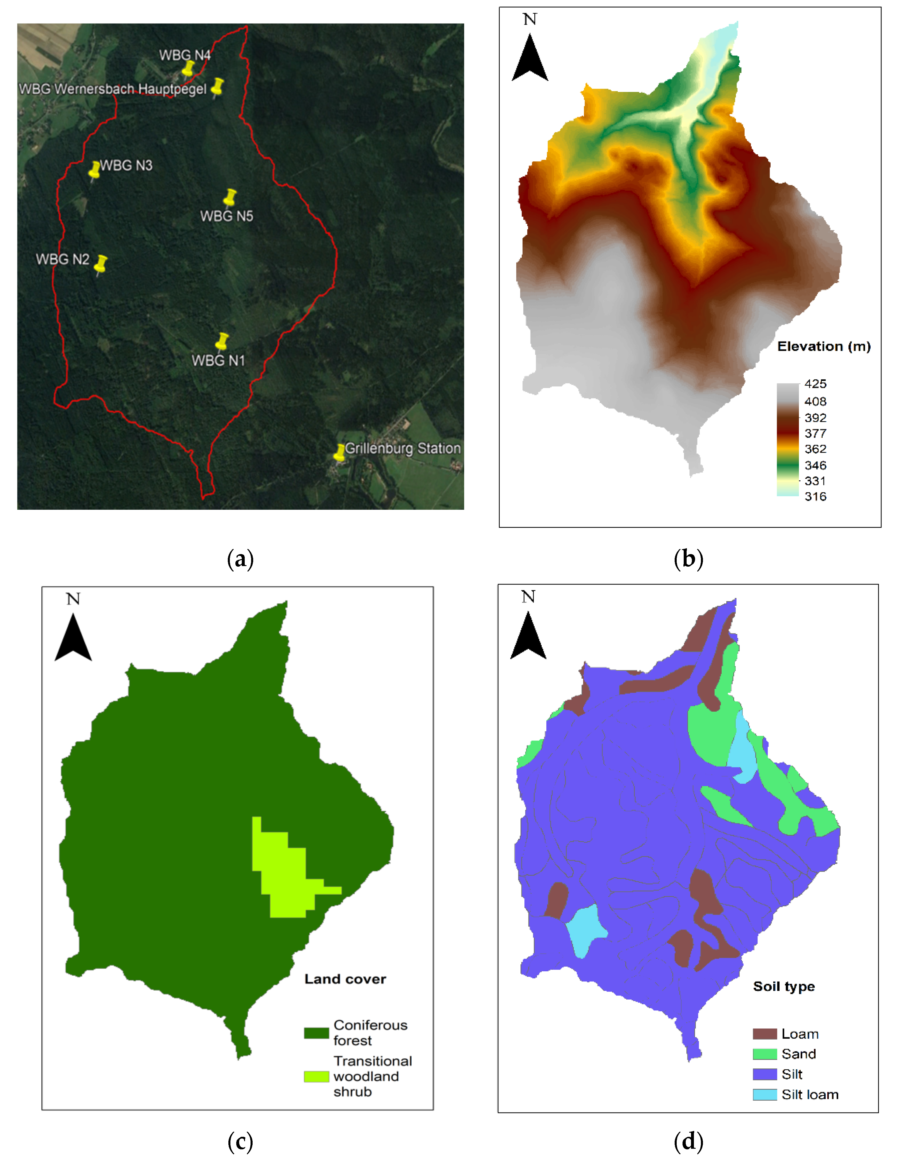
Figure 1. Location of data stations: (a) DEM, (b) land cover, (c) soil type, (d) maps of the Wernersbach catchment.
Hydrology 08 00109 g001
Figure 2. Map with the locations of data stations (a) and DEM (b) of the Wesenitz catchment.
Hydrology 08 00109 g002
Figure 3. Land cover (a) and soil type (b) maps of the Wesenitz catchment.
Hydrology 08 00109 g003
Figure 4. Hydrograph of the calibration year (1 October 2009–1 November 2010) for the Wernersbach catchment (1 soil layer). The red line illustrates the simulated flow, the black line represents the observed flow.
Hydrology 08 00109 g004
Figure 5. Hydrograph (a) and soil moisture (b) plots of the calibration year (1 October 2009–1 November 2010) with 2 soil layers for the Wernersbach catchment. The red line in the hydrograph illustrates the simulated flow, the black line represents the observed flow.
Hydrology 08 00109 g005aHydrology 08 00109 g005b
Figure 6. Flow duration curve for 1 soil layer (a) and 2 soil layers (b) of the calibration year (1 October 2009–1 November 2010) for the Wernersbach catchment.
Hydrology 08 00109 g006
Figure 7. Hydrograph (a) and soil moisture (b) plots of the calibration year (1 October 2012–1 November 2013) for the Wesenitz catchment. The red line in the hydrograph illustrates the simulated flow, the black line represents the observed flow.
Hydrology 08 00109 g007
Figure 8. Flow duration curve (a) and scatterplot (b) of the calibration year (1 October 2012–1 November 2013) for the Wesenitz catchment.
Hydrology 08 00109 g008
Figure 9. Hydrograph (a) and soil moisture (b) plots of the validation year (1 October 2012–1 November 2013) for the Wernersbach catchment. The red line in the hydrograph illustrates the simulated flow, the black line represents the observed flow.
Hydrology 08 00109 g009
Figure 10. Hydrograph of the highest flow in the period 2007–2014 with 1 soil layer (a) and 2 soil layer model (b) (25 May 2013–10 June 2013) for the Wernersbach catchment. The red line illustrates the simulated flow, the black line represents the observed flow.
Hydrology 08 00109 g010aHydrology 08 00109 g010b
Figure 11. Hydrograph (a) and soil moisture (b) plots of the validation year (1 October 2009–1 November 2010) for the Wesenitz catchment. The red line in the hydrograph illustrates the simulated flow, the black line represents the observed flow.
Hydrology 08 00109 g011
Table 1. Comparison of rainfall-runoff models.
NameMIKE-SHELisFLOODTopNETGeoTOPDREAMArnoTOPMODELTOPKAPI-X
Typephysically based, distributeddistributed, physically basedspatially distributed, conceptualdistributed, conceptualsemi-distributed, physically basedsemi-distributed, conceptualDistributed/semi-distributed, conceptualPhysically based, distributed
ETPPenman–Monteith method. Kristensen and Jensen methodPenman–Monteith methodPriestley–Taylor equationfunction of saturation-specific and atmospheric specific moisturePenman–Monteith based on air temperature and soil moisture, Radiation methodfunction of given potential ETP, air T and root zone moisture storageThornthwaite method
Runoff formationinfiltration excess and saturation excess flowDirect runoff and infiltration excessinfiltration excess and saturation excess flowinfiltration excess and saturation excess flowexfiltration from subsurface groundwater flowfunction of variable capacity of the soilinfiltration excess and saturation excess flowinfiltration excess and saturation excess flow
Groundwater saturated-2D Boussinesq equationparallel linear reservoirsfunction of topographic gradients3D Richards equationglobal linear reservoir modelNash modelDarcy’s Law1D Richards
Soil moisture balancefunction of rainfall, ETP, interflow etc.van Genuchten’s equationconcept of topographic indexCombination of heat and water flow equationsKirkby’s wetness indexTodini (1988) equationsteady state integral equationsfunction of several parameters
Infiltrationfunction of antecedent soil moistureSmith–Parlange methodgravity drainage and Green-Ampt3D Richards equationfunction of soil saturation capacityfunction of non-linear lawnon-linear reservoir functionsaturation excess
Interpolation Bilinear algorithmInverse distance methodDelauney triangles.KrigingThiessen polygonThiessen polygonstriangular weighting functionThiessen
Overland routing2D diffusive wave St.Venant equationfour-point finite difference solution of the kinematic wave with Manning equationreplaced by the time delay to simulate travel time in the basinkinematic scheme, which accounts for subgrid rilling and roughnessfunction of flowpath, relative flowtime and Manning equationusing linear parabolic modelsDistance related delay based on a constant overland flow velocity and routing distancekinematic wave approximation St.Venant equation
Channel routing1D full dynamic wave St.Venant equationfour-point finite difference solution of the kinematic wave with Manning equation1D Lagrangian kinematic scheme, Kinematic wave routingde Saint Venant parabolic equation using a constant celerityfunction of flowpath, relative flowtime and Manning equationusing linear/concentrated input parabolic modeldifferent routing options possible (e.g., constant velocity, gamma function)kinematic wave approximation St.Venant equation
References[44,45,46,47,48][49,50,51][33,52,53][54,55,56,57][58][59,60,61][62,63,64,65,66,67][32,68,69]
Table 2. Description of input data (format, source, etc.).
WernersbachWesenitz
Original DEM resolution (m)10 m30 m
D.E.M. sourceTU Dresden Institute of Hydrology and MeteorologyUSGS. Earth Explorer
DEM typeSatellite-basedSatellite-based
Land cover map formatshapefileshapefile
Land use map sourceEarth Observation centerEarth Observation center
Original scale of Land cover map1:100,000.1:100,000.
Soil type map formatshapefileshapefile
Soil cover map sourceFederal Institute for Geosciences and Natural ResourcesFederal Institute for Geosciences and Natural Resources
Original scale of Soil type map1:200,0001:200,000
Meteorological data sourceClimate Data Center of DWD.Climate Data Center of DWD.
Meteorological data time scaleHourlyDaily
Table 3. Land cover parameters for Wernersbach.
Land CoverManning’s nCrop Coefficients
123456789101112
Coniferous Forest0.127111111111111
Transitional Woodland Shrub0.058000.80.80.81110.950.9500
Table 4. Land cover parameters for Wesenitz.
Land CoverManning’s nCrop Coefficients
123456789101112
Discontinuous urban fabric0.115000.10.10.10.30.30.30.20.200
Industrial or commercial units0.23000.20.20.20.40.40.40.30.300
Mineral extraction sites0.104000.160.160.160.40.40.360.30.300
Sport and leisure facilities0.023000.10.10.10.30.30.30.20.200
Non-irrigated arable land0.043001.11.11.11.41.41.351.31.300
Pastures0.298000.40.40.40.90.90.90.80.800
Agricultural land with significant areas of natural vegetation0.058000.70.70.71.21.21.151100
Broad-leaved forest0.280.60.61.31.31.31.61.61.61.51.50.60.6
Coniferous forest0.22111111111111
Mixed forest0.280.80.81.21.21.21.51.51.51.31.30.80.8
Table 5. Calibrated soil parameters for Wernersbach.
Soil TypeKsh1Theta S1Theta R1Exp H1Ksh2Ksv2Theta S2Theta R2Exp H2Exp V2
Loam6.24 × 10−6–3.24 × 10−50.35–0.470.048–0.0581.2–1.82.4 × 10−6–2 × 10−54.49 × 10−9–1.24 × 10−80.4–0.430.05–0.081.2–1.518–25
Sand8.14 × 10−40.36–0.490.052.6–2.92.02 × 10−5–1.1 × 10−44.49 × 10−9–1.09 × 10−60.36-0.480.04–0.071.2–2.911.1–25
Silt4.3 × 10−6–6.6 × 10−50.38–0.50.039–0.0791.7–2.42.48 × 10−6–3.26 × 10−52.75 × 10−9–1.90 × 10−70.38-0.480.04–0.0551.2–2.911.1–25
Silt Loam4.7 × 10−50.340.0621.09 × 10−61.36 × 10−70.40.0492.911.1
Table 6. Calibrated soil parameters for Wesenitz.
Soil TypeKsh1Theta S1Theta R1Exp H1Ksh2Ksv2Theta S2Theta R2Exp H2Exp V2
Clay3.03 × 10−6–9.1 × 10−50.4–0.510.08–0.92.52.02 × 10−6–1.09 × 10−52.2 × 10−9–1.04 × 10−80.35–0.50.05–0.12.511.1–25
Loam1.86 × 10−6–9.28 × 10−50.4–0.50.05–0.92.51.24 × 10−6–6.07 × 10−51.1 × 10−9–5.67 × 10−80.38–0.470.035–0.12.511.1–25
Loamy Sand1.96 × 10−6–8.14 × 10−50.33–0.410.05–0.92.52.48 × 10−6–5.43 × 10−55.45 × 10−9–5.97 × 10−80.38–0.40.05–0.12.511.1–18
Sand1.63 × 10−4–5.96 × 10−40.31–0.510.035–0.82.55.43 × 10−5–2.17 × 10−49.95 × 10−9–1.19 × 10−70.35–0.50.05–0.12.511.1–25
Silt3.03 × 10−6–8.4 × 10−50.3–0.50.034–0.082.51.24 × 10−6–4.48 × 10−51.03 × 10−9–2.99 × 10−70.32–0.50.05–0.12.511.1–25
Silty Clay8.40 × 10−6–8.4 × 10−50.44–0.530.034–0.092.52.02 × 10−6–5.43 × 10−52.2 × 10−9–1.21 × 10−80.35–0.50.05–0.12.511.1–25
Silty Loam4.39 × 10−6–8.4 × 10−50.47–0.530.034–0.0852.51.24 × 10−6–9.9 × 10−51.36 × 10−9–7.7 × 10−70.25–0.50.05–0.12.511.1–25
Table 7. Goodness of fit test results for the calibration year of each catchment.
YearCatchmentMEMAERMSEPBIASNSEdR2KGEVE
2010Wernersbach
(1 layer)
−0.0130.030.05−220.830.950.730.760.53
2010Wernersbach
(2 layers)
−0.0060.020.04−100.890.970.870.880.64
2013Wesenitz−0.981.281.85−27.50.70.920.60.690.64
Table 8. Goodness of fit test results for the validation years of each catchment.
YearCatchmentMEMAERMSEPBIASNSEdR2KGEVE
2009Wernersbach−0.0020.0150.029−6.90.710.920.620.840.55
2012Wernersbach−0.0030.010.02−14.20.640.910.590.780.48
2013Wernersbach−0.0010.0210.058−1.40.950.990.940.970.69
2006Wesenitz−0.470.681.53−24.90.720.90.510.590.64
2008Wesenitz−0.090.70.88−4.30.670.930.790.730.66
2010Wesenitz−0.291.082.34−8.70.640.90.550.790.68
Publisher’s Note: MDPI stays neutral with regard to jurisdictional claims in published maps and institutional affiliations.