Abstract
Is sea level change affected by the presence of autocorrelation and abrupt shift? This question reflects the importance of trend and shift detection analysis in sea level. The primary factor driving the global sea level rise is often related to climate change. The current study investigates the changes in sea level along the US coast. The sea level records of 59 tide gauge data were used to evaluate the trend, shift, and persistence using non-parametric statistical tests. Mann-Kendall and Pettitt’s tests were utilized to estimate gradual trends and abrupt shifts, respectively. The study also assessed the presence of autocorrelation in sea level records and its effect on both trend and shift was examined along the US coast. The presence of short-term persistence was found in 57 stations and the trend significance of most stations was not changed at a 95% confidence level. Total of 25 stations showed increasing shift between 1990–2000 that was evaluated from annual sea level records. Results from the current study may contribute to understanding sea level variability across the contiguous US. This study extends an elaborative understanding of sea level trends and shifts which might be useful for water managers.
1. Introduction
According to the Intergovernmental Panel on Climate Change’s (IPCC) [] Fifth Assessment Report, the global sea level is estimated to rise 0.28–0.98 m by 2100 (1985–2005) in different representative concentration pathways scenario. Sea level in the Atlantic and Gulfs along US coasts have risen in the 20th century []. The local sea-level change may vary considerably from global sea level change due to factors such as land subsidence and emergence, global sea-level fluctuations, ocean circulation, and other localized factors. Sea level change in Sitka, Alaska is decreasing due to land emergence whereas Louisiana and Atlantic City are experiencing rising levels due to subsidence, which is unrelated to global sea level change according to the National Ocean and Atmospheric Administration website (NOAA, https://oceantoday.noaa.gov/globalvslocalsealevel/). Therefore, depending on the locations, and the rate over time it can cause spatial and temporal variability in sea level change [].
Most of the studies found an acceleration in sea level while some focused on sea-level deceleration. Houston and Dean [] found that during the 20th century the 57 US tide gage records did not show any acceleration. However, Rahmstorf and Vermeer [] disagreed with Houston and Dean [] and illustrated that using different start years for trend shows acceleration in sea level. The trend literatures corroborate that the hydroclimatological time series exhibit trends and the presence of autocorrelation [] might alter the significance of the trend. Furthermore, Meyssignac et al. [] state that internal climate variability has a dominant signal in the tropical Pacific than the anthropogenic forcing on regional sea level trends. This had led to an intensive debate in sea level studies and is also documented by Visser et al. []. To address these issues, detection of long-term sea level variability within the earliest record is essential to shaping our perspective of climate change as well as for policymakers to implement proper management plans to minimize the threat to the coastal ecosystems [,].
The increase in the rate of mean sea level is one of the main facets of probable climate variability and change []. The sea level natural variability is a non-stationary process that also drives sea-level fluctuations [,,]. Trend detection has been used widely for quantifying changes in hydroclimatological data. The trend detection of hydroclimatic data, which are non-stationary in nature, requires a robust statistical method that accounts for non-stationarity in time series []. Trends are estimated using both parametric and non-parametric tests. For most of the parametric tests, the time series are required to be normally distributed, which does not always apply to extreme events [].
Non-parametric tests are the most widely used and recommended technique due to their advantages that it does not assume any initial probability distribution and accounts for non-stationarity in the time series [,]. Therefore, the non-parametric Mann-Kendall (MK) test that requires independent data is highly beneficial for the trend estimation of hydroclimatic data. MK test is a rank-based robust approach, which is not sensitive to the distribution of the data, or the outliers, and is also efficient with missing data. However, it has some limitations on autocorrelated datasets. Yue et al. [] and Hamed and Rao [] corroborated that the trend significance was overestimated with the presence of positive autocorrelation whereas underestimated by negative autocorrelation in the time series. The hydroclimatic variables have a tendency to exist in clusters in a course of time, i.e., during extreme events; this is termed ‘scaling’ or ‘persistence’ []. These results are due to a lack of independence and are termed as short-term persistence (STP). The presence of one significant autocorrelation (lag-1) results in STP. Teegavarapu and Schmidt [] found strong autocorrelation in monthly sea level observations in US tide gages. In addition, Boon et al. [] also found the presence of autocorrelation in Washington DC tide gage and address the importance of removing significant autocorrelation for sea level trend estimation in Chesapeake Bay station in the United States. In addition, Becker et al. [] also used power law and corroborated that sea level change exhibits long-term correlations. Therefore, to evaluate the sea level trend within a time-series, the effects of STP should be carefully considered.
In geosciences, climate change and variability have created a need to detect persisting trends in gradual changes over a long historic period []. Similarly, studies have also detected sudden changes, which represent the abrupt changes in the hydroclimatological data []. Trends (gradual) are often observed throughout the time series and abrupt changes (shift) are the sudden changes that are due to non-homogeneity in the time series. Previously, Kerr [] and Trenberth and Hurrell [] demonstrated a sudden change during 1976–1977 in the Northern Pacific Ocean-atmosphere system which was later termed the climate regime shift of 1977 []. According to Villarini et al. [], categorizing trend (linear) and shift (non-linear) is essential as trend estimation can be affected by the shift in the data. Shift estimation is essential to understand whether the observed variation in the data is an effect of long-term variability, or a consequence of an abrupt shift []. Change-point analysis is done by utilizing a non-parametric Pettitt’s test that can detect the location of abrupt changes (shift) in the mean and variance in the time series. McCabe and Wolock [] also argued the presence of a trend might continue in the future. A trend typically follows a shift and time series may remain the same until another shift occur. Thus, a simultaneous study of both trend and shift is essential for the improved evaluation of the sea level variability. Moreover, evaluating the persistence while estimating the shift in the sea level would be an addition to the research gap.
The goal of the current study is to evaluate long-term sea level variability across the US coast by evaluating both gradual and abrupt changes in decadal scale. The study was motivated by the need to analyze whether the sea level is rising, falling, or exhibits no trend utilizing purely statistical approaches. The study addressed the following key questions (1) What is the overall sea level variability along the coastal US? (2) What is the significance of autocorrelation in both trend and shift? and (3) Does STP affect the local sea level trends around the USA? These research questions will assess the sea level change and the effects of autocorrelation on trend and shift. The major objectives of the current study are to (1) detect gradual changes by utilizing the MK test by considering autocorrelation for more realistic error statistics for the estimated trend parameters, and (2) detect abrupt shifts and confirm trend significance effects due to the presence of autocorrelation. Mann–Kendall test was performed in three ways to address the objective: (i) Mann–Kendall without autocorrelation (MK1), (ii) Mann–Kendall with lag-1 autocorrelation and trend-free pre-whitening (MK2), and (iii) Pettitt’s test to detect and evaluate the significance of the shift in the time series.
2. Materials and Methods
2.1. Study Area and Data
The latitude, longitude, and time-series data used in the current study are the in-situ water level measurements along the US coast acquired from the NOAA (https://tidesandcurrents.noaa.gov/stations.html?type=Water+Levels). The dataset used in this study represents the local relative sea level change. Out of 95 stations from NOAA, 59 stations were selected for this study on basis of the existing continuous data as shown in Figure 1. The monthly and annual raw data were obtained and the long-term data with the station having more than 30 continuous years of time-series data with no omission were used for the current study. For the analysis, the stations with maximum continuous time-series datasets were obtained. In total, 59 time-series were obtained with the station that had 70 years of data having a maximum record, while each gauge had at least 30 years of continuous time series. In this study, variable record length was used to cover maximum number of stations with more than 30 years of continuous records. The data from March to May is referred to as spring season, June to August as summer season, September to November as fall season, and December to February as winter season.
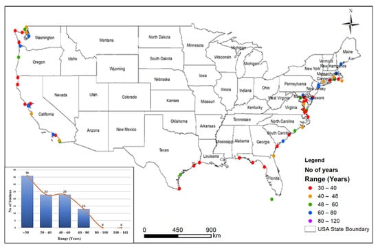
Figure 1.
Distribution of the number of tide gage station long the US coast with varying record length.
2.2. Methods
2.2.1. Trend Estimation Techniques
Variations in sea level can be estimated using a robust non-parametric MK test to determine the trend. The key advantages of the MK test are due to its accuracy working with a skewed distribution [,,,], and that it accounts for non-stationarity. In this test, each time series is ranked with reference to time in each station and test statistics S is computed. However, the MK test has limitations against autocorrelation resulting in spurious trends [,]. To account for this limitation, significant lag-1 autocorrelation significant at 90% was removed from the dataset to evaluate trends by utilizing pre-whitening to account for STP []. Persistence in a time-series results from an overestimation of a trend as an effect of an underestimated variance [,,]. Thus, considering the STP from the literature review is important, and was underlined in this study. A brief description of MK tests extracted from Yue et al. [] and Hamed [] is presented below:
The null hypothesis for the MK test states:
Hypothesis 1.
No trend.
Hypothesis 2.
Upward or Downward trend exists.
The test statistics S was obtained by using Equation (1) and function by Equation (2) below,
where
xk and xi are observations at a total length of time n. The variance of S is calculated using Equation (3).
The z test statistics is calculated using Equation (4).
The MK test is based on the null hypothesis that the time series has no trend. The direction (upward or downward) of the trend was determined by the MK test based on the obtained test statistics S sign (positive or negative). The significance level is given by test statistics z and determines the chances of rejecting the null hypothesis whereas confidence interval was calculated by subtracting significance level from 1.
A robust non-parametric method, Thiel-Sen approach (TSA) [,], is used in the current study to estimate the magnitude of trend. According to Sen [], it is effective with missing data and is also sensitive to outliers. It was computed using the β slope given in Equation (5). The estimate of the beta slope gives the rate of change to time. MK test without accounting for autocorrelation is referred to as MK1 hereafter.
The MK1 test has limitation to the presence of autocorrelation. To account this, the lag-1 autocorrelation coefficient (rk) was calculated using Equation (6).
The autocorrelation was removed by utilizing pre-whitening technique if the data lies outside the confidence level i.e., if data are found to be serially dependent. Else, trend free pre-whitening (TFPW) was applied as defined by Yue et al. []. The β slope was removed from the series to get detrended series by using Equation (7). Then, the lag-1 autocorrelation was removed from the detrended series by using Equation (8),
Then the trend is added back to the detrended series to get new series by using Equation (9). The MK test statistics S and z are again computed for the new series. MK test after accounting for autocorrelation is referred to as MK2 hereafter.
Separate MK1 test on each station was computed for annual and monthly time series and then MK2 were utilized independently to analyze the effects of short term persistence. Further, β slope on each station was also estimated separately for the different study period on the longest continuous available data.
2.2.2. Shift Detection
In addition to assessing the trend, abrupt changes were determined using the non-parametric Pettitt’s test []. It is a widely used test to analyze the non-homogeneity in the data. It is a rank-based approach and is less sensitive to outliers and skewness of the data. The Pettitt test evaluates the anomaly in mean within a time series at n length of time considering a shift at j years. It uses Mann-Whitney statistics to estimate the probability that the trends on either side of the shift at j years are significantly different by trials from the same population.
The test statistics are calculated using Equation (10).
where sgn(x) is a function defined in Equation (2) above.
The significant change point is obtained if test statistics |Uj,n| is maximum and is calculated using Equation (11), is the test statistics associated with the confidence level P.
At maximum |Uj,n|, the probability of shift is given by Equation (12),
If the significance level is more than the p-value, the null hypothesis is rejected, and a shift is detected. The direction of change also depends on the considered significance level; negative change indicates the minimum value, and the positive change indicates the maximum value.
Also, serial correlations were accounted for computing with and without TFPW in Pettitt’s test as proposed by Serinaldi and Kilsby [] to evaluate the existence of significant shifts in the dataset. Like trend, the time series were detrended by deducting the trend slope [] and removing the autocorrelation from the detrended dataset. This is the novel approach of the current study that makes the shift detection in sea level more reliable. Hence, with TFPW, the underlying trends can be detected, making Pettitt’s test more dependable. A 95% significance level (or p ≤ 0.05) was utilized to assess the significance of Pettitt’s test.
3. Results
3.1. Sea Level Trend and Persistence
The annual sea level trend analysis was performed to evaluate trends and persistence in sea level records. A total of 52 stations showed a positive trend, one showed negative and 6 showed no trend resulting from the MK1 test as shown in Table 1. The annual trend and slope were also obtained from the NOAA website (https://tidesandcurrents.noaa.gov/sltrends/mslUSTrendsTable.html) for comparison with the current study and shown in Figure 2a. The total number of stations obtained from NOAA website is 95 and in the current study, 59 stations with continuous time series were used. The time period of two stations used in this study is same as NOAA. NOAA records showed a decreasing trend in three stations in the Northwest. Of those, two stations showed no trend resulting from the MK1 test as shown in Figure 2b. Similarly, one station on the east coast and one station on the west coast showed no trend resulting from MK1 trend analysis whereas most of the stations showed a positive trend (Table 1). However, the magnitude of trends obtained from NOAA had similar range as that obtained from the MK1 test and is shown in Figure 2a,b. The STP was also accounted for annual sea level records to estimate the trend and analyze the effects of the presence of serial correlation on the trend estimation. The sea level trend evaluated after accounting for STP showed results like MK1 where most of the stations showed an increasing trend. Figure 2c shows the spatial plot of sea level trend after accounting for STP. From this, it can be observed that the significance of the trend of no station was changed to a non-significant trend. Instead, 52 stations showed a positive annual sea level trend, even after accounting for STP.

Table 1.
Summary of stations showing statistically significant monthly sea level trends at a 95% confidence level for tide gauges using MK1/MK2 test before/after autocorrelation and shift.
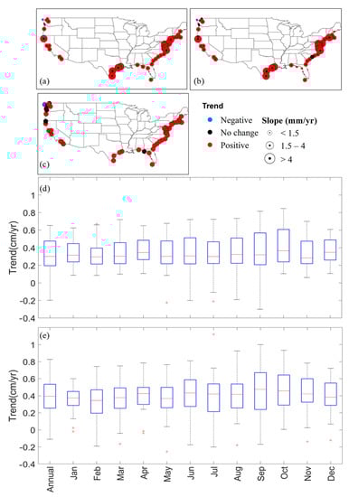
Figure 2.
Spatial plots showing the trend significance of annual sea level along the coastal US at the statistical significance of p ≤ 0.05 (a) National Ocean and Atmospheric Administration (NOAA) (b) Mann–Kendall without autocorrelation (MK1) trend. The trend is shown in red, blue, and black colors. The magnitude of the trend is represented by graduated symbols in (a,b). (c) Significance of annual trend after accounting short-term persistence (STP) (d) Box plots of the trend magnitudes corresponding to the sea level stations showing a significant MK1 trend (95% confidence level) for annual and all months (e) distribution of trend magnitude of latest available 30-year data. Each whisker shows the outliers, each red line shows the median, and each box represents the values within the 25th and 75th percentile of the sea level trend magnitude for each month. The positive (+) and negative sign (−) represents positive and negative trend respectively.
Table 1 shows the total number of stations with significant MK1 trends at a 95% confidence level for all months. Through the MK1 test, the sea level at 38 stations showed a significant positive trend. Furthermore, as observed, most of the stations showed an increasing trend for all months (Jan–Dec). The results indicate that the sea level trends of 40 stations exhibited a positive trend in March to November and 1 to 4 stations exhibited a negative trend in February, and May to September. July had the greatest number of positive trends (52, or 88%) followed by August having 51 stations, 50 stations in September, and 49 stations in October, whereas February had the fewest number of positive trends (33). The greatest number of significant negative monthly trends were in September (4), and the absence of negative trends was in January, March, April, October, November, and December. A significant positive trend with more than 40 stations was found in 9 months mostly located along the East Coast; however, more than 32 stations showed increasing trends every month. Table 1 shows the temporal sea level variation as increasing/positive, decreasing/negative, and no trend/no change along the US coast, at the 95% confidence level.
The magnitude of the trend was computed by utilizing the TSA slope for significant stations showing a trend at the level of significance, p ≤ 0.05. The maximum and minimum trend magnitude was 0.85 cm/year for October and 0.62 cm/year for January month, respectively as shown in Figure 2d using the entire dataset. Each whisker shows the outliers, each red line shows the median, and each box represents the values within the 25th and 75th percentile of the sea level trend magnitude for each month. The results of sea level indicate that the magnitude of sea-level starts increasing from May with slight fluctuations through September. It was noteworthy that the annual and monthly median was above zero. The maximum annual trend slope along the US coast was 0.64 cm/year whereas the minimum trend magnitude was −0.20 cm/year using the entire data.
Figure 2e shows the distribution of TSA slope by using the latest 30 years of available data from each station at different temporal scale (annual and monthly). The latest 30 years of data were used to observe the recent 30-year trend pattern in sea level because a minimum 30-year record is recommended to capture climate trends. It showed a similar range of trend magnitude that was obtained by using the entire dataset as shown in Figure 2d,e. The maximum annual trend slope along the US coast using the latest 30 years of available data was found to be 0.82 cm/year whereas the minimum trend magnitude was −0.11 cm/year. The 30-year trend magnitude was found to be 0.96 cm/year for September and 0.61 cm/year for January month.
The STP was accounted to estimate the monthly sea level trend and to assess the influence of presence of serial correlation on the significance of the trend estimation. The sea level trend evaluated with MK2 test showed similar results to MK1 as shown in Table 1. More than 28 stations showed significant trends after accounting for STP for all months as shown in Figure 3. Table 1 summarizes the total number of stations showing trends after accounting for STP. The highest lag-1 autocorrelation was observed in September and October having maximum stations with a positive trend (49 stations), followed by 39 stations in November. Out of 59 stations along the US coasts, the East Coast of the US had significant increasing trends throughout the year as observed from the spatio-temporal sea level variation from the MK1 test. Comparatively, the results accounting for STP indicated an increasing trend from summer through fall and decreasing from winter through spring with 48 stations showing an increasing trend in May. A maximum station showing a positive trend in sea level over the study period was observed for the spring season compared to the other seasons. The number of stations with an increasing trend increased from early spring—March (1 station)—through mid-fall—October (21 stations). The negative trend slowly reduced in winter with the least number of stations observed in February (1 station). Few stations showed a negative trend. From this, it can be observed that the trend significance of only a few stations was changed to a non-significant trend, whereas most of the stations showed a positive monthly sea level trend, even after accounting for STP, as shown in Table 1 and Figure 3.
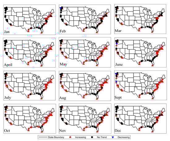
Figure 3.
Spatial plots showing the MK2 trend significance of monthly sea level along the coastal US accounting STP. The red upward arrow represents an increasing/positive trend whereas the blue downward arrow represents a decreasing/negative trend. The black dot represents stations showing no trend at the statistical significance of p ≤ 0.05.
3.2. Shift Detection in Sea Level
Thirty-eight out of 59 stations showed a significant positive abrupt change in January and 21 stations showed no shift in the data. The maximum number of stations showing a positive shift was 52 (88%) in May, before accounting for autocorrelation, and August, both before and after accounting for autocorrelation (Table 1). However, for May only 3 stations showed a negative shift and 4 stations in September both before and after accounting autocorrelation. The Pettitt test results identified that the shift years clustered from the 1960s to 2012. The maximum significant negative shift was found in four stations in September. Most of the increasing shifts were found between 1991 and 2000 as shown in Table 2. A maximum number of stations showed a positive shift from May through October. A few stations in some months experienced a shift earlier in the year. Along with the trend, it showed an increase in the presence of abrupt changes. Furthermore, Pettitt’s test was also performed in annual sea level record and it was observed that 25 stations showed a shift between 1991–2000 as shown in Table 2. Figure 4a,b represents the spatial maps showing shift year before and after accounting autocorrelation in the shift. It can be noted that the nearby stations have a similar shift year. From Figure 4c it is evident that 57 stations out of 59 stations show the presence of lag-1 autocorrelation.
Table 2.
Number of stations in different months at different time intervals and four seasons showing shifts.
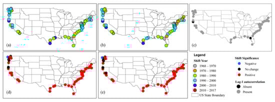
Figure 4.
Spatial plots showing the results for the shift of annual sea level along the coastal US. Represents (a) Shift year before accounting for autocorrelation (b) Shift year after accounting for autocorrelation (c) Lag-1 autocorrelation (d) Shift significance year before accounting for autocorrelation (e) Shift significance year after accounting for autocorrelation. The red circle represents an increasing/positive trend whereas the blue downward arrow represents a decreasing/negative trend. The black dot represents stations showing no trend at the statistical significance of p ≤ 0.05.
The step with pre-whitening was also utilized to consider the effects of serial correlation on the Pettitt test on the monthly and annual sea level records. The shift was investigated after accounting for serial correlation and the overall similar pattern of the shift was observed when compared with shift before accounting for autocorrelation. However, few stations had different shifts years after accounting for serial correlation in the Pettitt test in a few months as shown in Figure 4b. Overall, the abrupt shift analysis confirms that the effects of STP on the stations and the significance of only a few stations changed after applying the TFPW in the shift test. In addition, 53 out of 59 stations showed a positive shift before accounting for autocorrelation whereas 52 stations after accounting for autocorrelation resulted from shift analysis in annual sea level record as shown in Table 1. The spatial plot of shift significance before and after accounting autocorrelation at 95% confidence level is shown in Figure 4d,e respectively.
Most of the shifts occurred during fall, winter, and summer between 1991–2000. Alternatively, during the spring most shifts occurred between 1971–1980. During 1991–2000, 46 out of 59 stations showed a positive shift in fall, 41 out of 59 stations showed a positive shift in winter, and 40 out of 59 stations showed a positive shift in summer. Only 5 out of 59 showed the presence of a shift in the spring. Similarly, during 1971–1980, 27 out of 59 showed shifts in fall, 17 out of 59 stations showed a shift in winter, 22 out of 59 stations showed a shift in summer (Table 2). Only 11 out of 59 showed the presence of shift in spring, respectively. From this, we can infer that during spring the minimum number of stations exhibiting a shift was observed (only 1) with 11 stations being the maximum during that interval.
4. Discussion
Both MK and Pettitt’s test works well on distribution-free time series thus, autocorrelation was tested in the current study, and if present, autocorrelation was removed with the TFPW technique as suggested by Yue et al. [] and Hamed []. The presence of autocorrelation was identified before evaluating trend and shift for precise estimation of sea level change. The presence of autocorrelation alters the variance of the distribution. Serinaldi and Kilsby [] emphasized the importance of incorporating the serial correlation for shift detection. The characteristics and statistical significance of these serial correlations and their effects on the sea level variability have not been identified in previous studies. In the current study, the long-term trend was analyzed to examine the persistence as it can pose significant deviations and affect the local trends. The inclusion of persistence was also useful to address evidence to different real and spurious trends [].
This study also provides strong scientific evidence that the assumption of stationarity while assessing sea level trends may not be valid. The MK and Pettitt’s tests are widely used as it accounts for non-stationary behavior in time series. The sea level was observed to have STP at most of the stations. In this study, both STP and the abrupt shift were detected which signifies the presence of non-stationarities in the dataset. The lag-1 autocorrelation was considered to remove significant autocorrelation in the sea level to correctly evaluate the variation in the sea level. The presence of STP in the data does not alter the magnitude of trends, but it significantly reduced the statistical significance of the trends in Kumar et al.’s research []. Previous studies have shown that the z-value of MK tests was significantly reduced after incorporating STP for annual flow statistics [] temperature, precipitation, and streamflow []. However, in this study, it was observed that statistically significant sea level trends may not be statistically significant after accounting for the STP in only a few stations as shown in Table 1. Most stations on the East Coast exhibited an increasing trend, even after considering the STP.
The significance of autocorrelation was tested in the trend and shift detection and it was observed that the significance of trend did not change in most of the stations, even after accounting for the autocorrelation in annual and monthly sea level record as shown in Table 1, and Figure 2. A possible mode of non-stationarity was presented by using the shift analysis. Teegavarapu [] also states the importance of considering the abrupt shift in sea level trend analysis. The time-series detecting shift and autocorrelation was the main focus of the current study to estimate the temporal trend as suggested by Teegavarapu []. The detection of shift showed that the variation in the sea level is also affected mostly by the shift in the data in addition to the long-term gradual changes as trends. Further, the analysis shows that the presence of autocorrelation in a significant shift does not change the trend significance in most of the stations as shown in Figure 3 and Table 1. In the future, another trend in the sea level may be observed with another abrupt shift in the data.
The 1970s shift years detected in this study are well documented in previous studies []. Further, Woodsworth et al. [] also found positive acceleration related to an ‘inflexion’ point in the US tide gages in 1930. The determination of time of occurrence of sudden changes in time series aids researchers to find the evidence of natural or anthropogenic changes in climatic, hydrologic, or land use. In addition, the abrupt shift could also be due to non-homogeneity in the dataset which is often affected by the moving of the stations. The significant shift years also represent non-stationary behavior in sea level records. Therefore, it is very important to identify the period from where significant change has occurred in sea level record. In the current study, summer season showed a maximum of the station showing a shift in all categorized years with a maximum of 40 stations in 1991–2000. However, few nearby stations are observed in the different shift year range which could be due to the variable record length used in this study.
The World Meteorological Organization (WMO) [] noted the unprecedented decadal rise of temperature in 1991–2000 and 2001–2010. The sea surface temperature is high during the summer and 1991–2000 was warm due to increased temperatures [,,]. This may have increased the positive sea level trend as the current study observed a higher number of stations showing a shift during 1991–2000. Reager et al. [] observed that sea-level rise has been slowed due to climate-driven processes and human activities. It is also discussed by Chao et al. [] that water management in the reservoir could be one of the factors of slow sea level rise and found that the trend since 1930 would be almost linear than deceleration. The results of abrupt changes could be due to variation in gauging practices, land-use change, and regulations of rivers by reservoir operations, water management implementations as well as being an indication of the severity of a climate event. Also, the shift could be due to anthropogenic processes like water pumping, urbanization, terrestrial water storage changes, and storm surges which have not been considered in the current study and could be a potential area for future research.
5. Conclusions
Previous studies on sea level changes suggest both an increase and a decrease in sea level, whereas in this study the trend was found to be significant at 95% confidence level, even after accounting for autocorrelation. The current study intends to analyze both trends and shift at both spatial and temporal scales along the contiguous US coasts. The abrupt and gradual changes in sea level utilizing the available tide gauge (30–70-year record) dataset were analyzed in this study. The current study focused on long-term changes as trend and abrupt shift in monthly and annual sea level along the US coast.
Persistence at short-term temporal scales was considered to estimate its effects in both trend and shift. The study accounted for lag-1 autocorrelation to confirm STP. The key conclusions from the present analysis can be summarized as:
- The gradual trend analysis revealed the presence of STP in most of the stations and it is evident that most stations show a positive sea level trend, even after accounting autocorrelation. The maximum and minimum trend magnitude that was evaluated by using the entire dataset was found to be 0.85 cm/year for October and 0.62 cm/year for January, respectively.
- Previous studies focused on gradual trends while the current study is unprecedented as it considers the presence of both gradual and abrupt changes in sea level.
- The autocorrelation in sea level can significantly change the detection of a sea level trend and shift. However, the most of stations showed a positive trend before and after accounting for the autocorrelation. Accounting for autocorrelation yielded more reliable results.
- The number of stations showing significant shifts was similar after accounting for autocorrelation in sea level records. In the annual time series, 53 stations showed an increasing trend before autocorrelation, and 52 stations showed an increasing shift, even after the accounting of the autocorrelation in the shift.
- This study concludes that the presence of autocorrelation did not change the significance of trend and shift in most stations. Most stations showed increasing trend and shift after accounting for autocorrelation.
This study identified the shift years and influential seasons within the spatial distribution of stations undergoing significant shifts. These results could be useful to understand the behavioral change in each station. Additionally, this study is intended for future research in how we understand sea level changes, and is also beneficial for coastal water management.
Author Contributions
Conceptualization, A.K.; Investigation, N.J.; Software, N.J.; Formal analysis, N.J. and B.T.; Supervision, A.K.; Writing—original draft preparation, N.J., A.K. and K.W.L.; Writing—review and editing, N.J., A.K., B.T., S.B. and K.W.L. All authors have read and agreed to the published version of the manuscript.
Funding
This research received no external funding.
Institutional Review Board Statement
Not applicable.
Informed Consent Statement
Not applicable.
Data Availability Statement
The data can be accessed in NOAA’s website.
Acknowledgments
The authors would like to thank the editor and four anonymous reviewers for constructive feedback. The authors would like to acknowledge the Dissertation Research Assistantship Award provided by the graduate school at Southern Illinois University, Carbondale.
Conflicts of Interest
The authors declare no conflict of interest.
References
- IPCC. Climate Change and the Ocean: Special Collection of Reprints from the Working Group II Contribution to the Fifth Assessment Report of the Intergovernmental Panel on Climate Change; Intergovermental Panel of Climate Change; Cambridge University Press: Cambridge, UK; New York, NY, USA, 2014; p. 1820. Available online: https://www.ipcc.ch/site/assets/uploads/2018/03/WGII-AR5_Oceans-Compendium.pdf (accessed on 19 July 2019).
- Titus, J.G.; Richman, C. Maps of lands vulnerable to sea level rise: Modeled elevations along the US Atlantic and Gulf coasts. Clim. Res. 2001, 18, 205–228. [Google Scholar] [CrossRef]
- Vecchio, A.; Anzidei, M.; Serpelloni, E.; Florindo, F. Natural Variability and Vertical Land Motion Contributions in the Mediterranean Sea-Level Records over the Last Two Centuries and Projections for 2100. Water 2019, 11, 1480. [Google Scholar] [CrossRef]
- Houston, J.R.; Dean, R.G. Sea-Level Acceleration Based on U.S. Tide Gauges and Extensions of Previous Global-Gauge Analyses. J. Coast. Res. 2011, 27, 409–417. [Google Scholar] [CrossRef]
- Rahmstorf, S.; Vermeer, M. Discussion of: Houston, J.R.; Dean, R.G. Discussion of: Houston, J.R. and Dean, R.G., 2011. Sea-Level Acceleration Based on U.S. Tide Gauges and Extensions of Previous Global-Gauge Analyses. “Journal of Coastal Research”, 27(3), 409–417. J. Coast. Res. 2011, 27, 784–787. [Google Scholar] [CrossRef]
- Cohn, T.A.; Lins, H.F. Nature’s style: Naturally trendy. Geophys. Res. Lett. 2005, 32. [Google Scholar] [CrossRef]
- Meyssignac, B.; Salas, D.; Becker, M.; Llovel, W.; Cazenave, A. Tropical Pacific spatial trend patterns in observed sea level: Internal variability and/or anthropogenic signature? Clim. Past Discuss. 2012, 8, 787–802. [Google Scholar] [CrossRef]
- Visser, H.; Dangendorf, S.; Petersen, A.C. A review of trend models applied to sea level data with reference to the “acceleration-deceleration debate”. J. Geophys. Res. Oceans 2015, 120, 3873–3895. [Google Scholar] [CrossRef]
- Nicholls, R.J.; Cazenave, A. Sea-Level Rise and Its Impact on Coastal Zones. Science 2010, 328, 1517–1520. [Google Scholar] [CrossRef]
- Epanchin-Niell, R.; Kousky, C.; Thompson, A.; Walls, M. Threatened protection: Sea level rise and coastal protected lands of the eastern United States. Ocean Coast. Manag. 2017, 137, 118–130. [Google Scholar] [CrossRef]
- Hausfather, Z. Explainer: How Climate Change Is Accelerating Sea Level Rise. CarbonBrief. 2019. Available online: https://www.carbonbrief.org/explainer-how-climate-change-is-accelerating-sea-level-rise (accessed on 31 October 2019).
- Han, W.; Stammer, D.; Meehl, G.A.; Hu, A.; Sienz, F.; Zhang, L. Multi-Decadal Trend and Decadal Variability of the Regional Sea Level over the Indian Ocean since the 1960s: Roles of Climate Modes and External Forcing. Climate 2018, 6, 51. [Google Scholar] [CrossRef]
- Joshi, N.; Kalra, A.; Lamb, K.W. Land–Ocean–Atmosphere Influences on Groundwater Variability in the South Atlantic–Gulf Region. Hydrology 2020, 7, 71. [Google Scholar] [CrossRef]
- Tamaddun, K.; Kalra, A.; Ahmad, S. Identification of streamflow changes across the continental United States using variable record lengths. Hydrology 2016, 3, 24. [Google Scholar] [CrossRef]
- Qian, C.; Zhou, W.; Fong, S.K.; Leong, K.C. Two Approaches for Statistical Prediction of Non-Gaussian Climate Extremes: A Case Study of Macao Hot Extremes during 1912–2012. J. Clim. 2015, 28, 623–636. [Google Scholar] [CrossRef]
- Karthikeyan, L.; Kumar, D.N. Predictability of nonstationary time series using wavelet and EMD based ARMA models. J. Hydrol. 2013, 502, 103–119. [Google Scholar] [CrossRef]
- Thakur, B.; Kalra, A.; Joshi, N.; Jogineedi, R.; Thakali, R. Analyzing the Impacts of Serial Correlation and Shift on the Streamflow Variability within the Climate Regions of Contiguous United States. Hydrology 2020, 7, 91. [Google Scholar] [CrossRef]
- Yue, S.; Pilon, P.; Phinney, B.; Cavadias, G. The influence of autocorrelation on the ability to detect trend in hydrological series. Hydrol. Process. 2002, 16, 1807–1829. [Google Scholar] [CrossRef]
- Hamed, K.H.; Rao, A.R. A modified Mann-Kendall trend test for autocorrelated data. J. Hydrol. 1998, 204, 182–196. [Google Scholar] [CrossRef]
- Bunde, A.; Havlin, S.; Koscielny-Bunde, E.; Schellnhuber, H.J. Long term persistence in the atmosphere: Global laws and tests of climate models. Phys. A Stat. Mech. Appl. 2001, 302, 255–267. [Google Scholar] [CrossRef]
- Teegavarapu, R.S.; Schmidt, A.R. Variations and Trends in Global and Regional Sea Levels. In Trends and Changes in Hydroclimatic Variables; Elsevier: Cambridge, MA, USA, 2019; pp. 361–401. [Google Scholar] [CrossRef]
- Boon, J.D.; Brubaker, J.M.; Forrest, D.R. Chesapeake Bay Land Subsidence and Sea Level Change: An Evaluation of Past and Present Trends and Future Outlook; Special Report in Applied Marine Science and Ocean Engineering; Virginia Institute of Marine Science: Gloucester Point, VA, USA, 2010. [Google Scholar] [CrossRef]
- Becker, M.; Karpytchev, M.; Lennartz-Sassinek, S. Long-term sea level trends: Natural or anthropogenic? Geophys. Res. Lett. 2014, 41, 5571–5580. [Google Scholar] [CrossRef]
- Mahmood, R.; Jia, S.; Zhu, W. Analysis of climate variability, trends, and prediction in the most active parts of the Lake Chad basin, Africa. Sci. Rep. 2019, 9, 1–18. [Google Scholar] [CrossRef]
- Mantua, N.J.; Hare, S.R. The Pacific Decadal Oscillation. J. Oceanogr. 2002, 58, 35–44. [Google Scholar] [CrossRef]
- Kerr, R.A. Unmasking a shifty climate system. Science 1992, 255, 1508. Available online: https://www.jstor.org/stable/2876764 (accessed on 18 September 2019). [CrossRef] [PubMed]
- Trenberth, K.E.; Hurrell, J.W. Decadal atmosphere-ocean variations in the Pacific. Clim. Dyn. 1994, 9, 303–319. [Google Scholar] [CrossRef]
- Powell, A.M., Jr.; Xu, J. The 1977 Global Regime Shift: A Discussion of Its Dynamics and Impacts in the Eastern Pacific Ecosystem. Atmos. Ocean 2012, 50, 421–436. [Google Scholar] [CrossRef]
- Villarini, G.; Serinaldi, F.; Smith, J.A.; Krajewski, W.F. On the stationarity of annual flood peaks in the continental United States during the 20th century. Water Resour. Res. 2009, 45. [Google Scholar] [CrossRef]
- McCabe, G.J.; Wolock, D.M. A step increase in streamflow in the conterminous United States. Geophys. Res. Lett. 2002, 29, 38. [Google Scholar] [CrossRef]
- Kalra, A.; Piechota, T.; Davies, R.; Tootle, G.A. Changes in U.S. Streamflow and Western U.S. Snowpack. J. Hydrol. Eng. 2008, 13, 156–163. [Google Scholar] [CrossRef]
- Önöz, B.; Bayazit, M. The power of statistical tests for trend detection. Turk. J. Eng. Environ. Sci. 2003, 27, 247–251. [Google Scholar]
- Wahl, T.; Jensen, J.; Frank, T.; Haigh, I.D. Improved estimates of mean sea level changes in the German Bight over the last 166 years. Ocean Dyn. 2011, 61, 701–715. [Google Scholar] [CrossRef]
- Barbosa, S.M.; Silva, M.E.; Fernandes, M.J. Time series analysis of sea-level records: Characterising long-term variability. In Nonlinear Time Series Analysis in the Geosciences; Springer: Berlin/Heidelberg, Germany, 2008; pp. 157–173. [Google Scholar] [CrossRef]
- Kumar, S.; Merwade, V.; Kam, J.; Thurner, K. Streamflow trends in Indiana: Effects of long term persistence, precipitation and subsurface drains. J. Hydrol. 2009, 374, 171–183. [Google Scholar] [CrossRef]
- Von Storch, H. Misuses of Statistical Analysis in Climate Research. In Analysis of Climate Variability; Springer: Berlin/Heidelberg, Germany, 1999; pp. 11–26. [Google Scholar] [CrossRef]
- Hamed, K.H. Trend detection in hydrologic data: The Mann–Kendall trend test under the scaling hypothesis. J. Hydrol. 2008, 349, 350–363. [Google Scholar] [CrossRef]
- Thiel, H. A rank-invariant method of linear and polynomial regression analysis, Part 3. In Proceedings of the Koninalijke Neder-landse Akademie van Weinenschatpen A, 30 September 1950; Available online: https://www.dwc.knaw.nl/DL/publications/PU00018789.pdf (accessed on 11 December 2020).
- Sen, P.K. Estimates of the regression coefficient based on Kendall’s Tau. J. Am. Stat. Assoc. 1968, 63, 1379–1389. [Google Scholar] [CrossRef]
- Pettitt, A.N. A Non-Parametric Approach to the Change-Point Problem. J. R. Stat. Soc. Ser. C Appl. Stat. 1979, 28, 126. [Google Scholar] [CrossRef]
- Serinaldi, F.; Kilsby, C.G. The importance of prewhitening in change point analysis under persistence. Stoch. Environ. Res. Risk Assess. 2015, 30, 763–777. [Google Scholar] [CrossRef]
- Miller, W.P.; Piechota, T.C. Regional Analysis of Trend and Step Changes Observed in Hydroclimatic Variables around the Colorado River Basin. J. Hydrometeorol. 2008, 9, 1020–1034. [Google Scholar] [CrossRef]
- Kalra, A.; Sagarika, S.; Pathak, P.; Ahmad, S. Hydro-climatological changes in the Colorado River Basin over a century. Hydrol. Sci. J. 2017, 62, 2280–2296. [Google Scholar] [CrossRef]
- Teegavarapu, R.S. Methods for Analysis of Trends and Changes in Hydroclimatological Time-Series. In Trends and Changes in Hydroclimatic Variables; Elsevier: Cambridge, MA, USA, 2019; pp. 1–89. [Google Scholar] [CrossRef]
- Lehmann, A.D.; Getzlaff, K.; Harlaß, J. Detailed assessment of climate variability in the Baltic Sea area for the period 1958 to 2009. Clim. Res. 2011, 46, 185–196. [Google Scholar] [CrossRef]
- Woodworth, P.L.; White, N.J.; Jevrejeva, S.; Holgate, S.J.; Church, J.A.; Gehrels, W.R. Evidence for the accelerations of sea level on multi-decade and century timescales. Int. J. Clim. 2008, 29, 777–789. [Google Scholar] [CrossRef]
- WMO. Climate 2001–2010: A Decade of Climate Extremes—Summary Report; WMO No. 1119; World Meteorological Organization: Geneva, Switzerland, 2013. [Google Scholar]
- Shrestha, A.; Rahaman, M.; Kalra, A.; Jogineedi, R.; Maheshwari, P. Climatological Drought Forecasting Using Bias Corrected CMIP6 Climate Data: A Case Study for India. Forecasting 2020, 2, 4. [Google Scholar] [CrossRef]
- Thakur, B.; Kalra, A.; Lakshmi, V.; Lamb, K.W.; Miller, W.P.; Tootle, G. Linkage between ENSO phases and western US snow water equivalent. Atmos. Res. 2020, 236, 104827. [Google Scholar] [CrossRef]
- Reager, J.T.; Gardner, A.S.; Famiglietti, J.S.; Wiese, D.N.; Eicker, A.; Lo, M.-H. A decade of sea level rise slowed by climate-driven hydrology. Science 2016, 351, 699–703. [Google Scholar] [CrossRef] [PubMed]
- Chao, B.F.; Wu, Y.H.; Li, Y.S. Impact of Artificial Reservoir Water Impoundment on Global Sea Level. Science 2008, 320, 212–214. [Google Scholar] [CrossRef] [PubMed]
Publisher’s Note: MDPI stays neutral with regard to jurisdictional claims in published maps and institutional affiliations. |
© 2021 by the authors. Licensee MDPI, Basel, Switzerland. This article is an open access article distributed under the terms and conditions of the Creative Commons Attribution (CC BY) license (http://creativecommons.org/licenses/by/4.0/).