Assessment of Surface Irrigation Potential of the Dhidhessa River Basin, Ethiopia

Abstract

Assessing available water resources and their potential for irrigation water use is vital for sustainable agricultural development and planning. This is particularly of interest in developing countries like Ethiopia, where a small portion of largely accessible land for surface irrigation applications has been utilized, despite the majority of the population relying on agricultural productivity. This study utilized the Dhidhessa River Basin (Ethiopia) as a case study and analyzed the main challenges to balance the sustainable water resources utilization and enhance agricultural productivity of the basin. The study mainly focused on estimating the available water resources and their potential for surface irrigation water use in the basin. This was achieved by utilizing Geographic Information System (GIS)-based tools, a hydrological Soil and Water Assessment Tool (SWAT) model, and a Crop Water and Irrigation Requirements Program of FAO (CROPWAT) model. While the SWAT estimated the water availability in the basin, GIS-tools such as Model Builder were used to map the irrigation potential of the basin. For irrigation water potential assessment, we selected six crops (cabbage, maize, tomato, pepper, groundnut and sugarcane) and estimated their irrigation water requirements using the CROPWAT model. We developed the SWAT model for the period from 1986 to 2012 using the available hydro-meteorological and geo-spatial data. Due to many parameters used in the model, we first performed a parameter sensitivity analysis and identified the most essential/sensitivity parameters via Sequential Uncertainty Fitting-II (SUFI-2). The identified sensitive parameters were subsequently used for model calibration (1989–2000) and validation (2001–2012) procedures achieved via SUFI-2. SWAT was able to reproduce the observed monthly streamflow values with a coefficient of determination (R²) and Nash-Sutcliffe Coefficient (NSE) of 0.85 and 0.87 for the calibration period and 0.91 and 0.89 for the validation period, respectively. The findings generally indicated a “good” performance of the model in simulating the hydrology. The annual available water of the basin is 9.26 billion cubic meters (BCM) whereas the 70% and 80% dependable flow is 7.56 and 6.97 BCM, respectively. Based on the Model Builder of ArcGIS, the SWAT estimated available water can potentially irrigate an area of 259,028 ha for slope less than 8%, 643,162 ha for slopes less than 15% and 1,023,581 ha for slopes less than 30%. Moreover, the irrigation water requirements were calculated by the CROPWAT model for the six selected crops indicated that although the need for irrigation water varies depending on the season, the potential irrigation area of the Dhidhessa River Basin is greater than its irrigated land. Therefore, it is concluded that the basin’s surface irrigation systems need to be expanded to enhance the agricultural productivity and improve the livelihood of the basin’s communities and similar basins elsewhere.

1. Introduction

Due to population growth and increases in firewater resource demand, it has been become a challenge to sustain the unevenly distributed water resources worldwide [1]. In addition, the geo-morphological conditions and climate change/variability have further exacerbated freshwater availability and thus increases its demand, both temporally and spatially [1,2,3]. Globally, climate change has been putting pressure on the problem, modifying hydrological responses and shifts in time of rainfall-runoff responses [1,4,5]. Consequently, it has been documented that about two-thirds of the world’s population have been, or will be, suffering from water shortage or unavailability [1,6,7]. These negative implications have been more pronounced in developing countries that mainly depend on rain-fed agricultural systems. Thus, such countries, including Ethiopia, may need to migrate from the traditional agricultural practices towards irrigation-based systems [8]. However, the amount of water available for irrigation depends on the availability of freshwater resources [9,10,11,12,13]. At the same time, agricultural areas have also been further threatened by the expansion of the residential and development areas, commercial/industrials, and other sectors [14,15].

Some studies have already shown the negative and potential impact of climate change on water resources supply for agriculture, urbanization, and other environment uses [1,16,17,18]. While both groundwater and surface water are very susceptible to climate change [16,17,19,20,21], some researchers have reported that there is a limited understanding of the dynamic relationship between groundwater and climate change [19,22]. In addition, the impact of climate change could be intensified by human interference such as irrigation water use and land use change [19,22]. Therefore, the world has been facing the problem of tackling the impact of climate and land use changes, population growth and urbanization on water resources and agricultural production and products [16,23].

The available water from surface water, renewable groundwater, and rainwater can be used for agriculture and irrigation [24,25,26]. However, such water sources have been severely under-developed and under-utilized in Ethiopia, implying the importance of enhancing the irrigation water potential of the available water resources [27,28]. Ethiopia mainly depends on rain-fed agriculture with limited use of irrigation for agricultural production [29]. Approximately >85% of the country’s food supply has been generated from rain fed agriculture and low-productive subsistence crops [30]. Hence, rainfall is the most determining factor for food production, supply and the economy of the country [30]. However, increases in temperature and the alteration of rainfall patterns in Ethiopia have direct effects on agricultural crop growth and yields [31,32,33]. The major problem associated with rainfall-dependent agriculture in the country is the high degree of rainfall variability and unreliability [34,35]. Such conditions might cause crop failures due to the frequent occurrence of dry spells and droughts. This in turn often results in famine, particularly affecting the livelihoods of the rural and poor communities. Consequently, food and nutrition insecurity are a frequent and bottleneck problem in Ethiopia. Therefore, the country needs alternative approaches, for example enhancing irrigation water use from its abundant rivers, such as the Dhidhessa River Basin (DRB), and thus improving the agricultural productivity of the rural and poor communities [36].

The Dhidhessa River is one of the biggest tributaries of the upper Blue Nile River (the Abbay River in Ethiopia) [37]. The Dhidhessa River accounts for approximately about one-fourth of the Blue Nile River (BNR) [38,39,40,41,42]. Given its major contributions to the BNR, the Dhidhessa River can be considered as one of the potential water resources to alleviate agricultural productivity and food security problems through the use of advanced irrigation systems [38]. The land and water resource potential assessment using hydrological models has been important to ensure the sustainable development [43,44,45]. On the other hand, the evaluation of basin irrigation potential and irrigation water requirement is crucial in order to enhance food security [2,31,46,47,48,49]. Previous studies have proven the applicability of the Soil and Water Assessment Tool (SWAT) model for irrigation potential assessment of the BNR Basins even with limited data [50,51,52]. SWAT is an open access and widely used model in poorly gauged basins like the BNR basin [50,52,53]. For example, the irrigation potential of Lake Tana, which is one of the contributors to the BNR, was extensively studied compared to the other sub basins of the BNR [54,55,56,57,58]. Although the Dhidhessa River Basin has comparatively sufficient hydrological and meteorological time series data (compared to the other sub-basins of the BNR), its hydrological and land resource development have not been well investigated yet. More specifically, the basin has not been well studied and understood as compared with the northern sub-basins of the Blue Nile River such as Tana sub-basin. There is limited information regarding the water resources development and surface irrigation potential of the Dhidhessa River Basin. There is a need to secure food security and water resource development in the country. The potential irrigation assessment is the first step towards ensuring sound planning and sustainability of irrigation development and ultimately to secure food and nutrition security [59]. Hence, this study was performed using the Soil and Water Assessment Tool (SWAT) and GIS as a tool for assessing the irrigation potential in the Dhidhessa River sub-basin. Furthermore, the study attempted to estimate the water resource potential of the river catchments in the basin and identify irrigable areas. The objective of this study is to demonstrate the available resources of the basin for sustainable development. As such, irrigation potential assessment is the first step towards ensuring planning and suitability of irrigation development in the area.

2. Materials and Methods

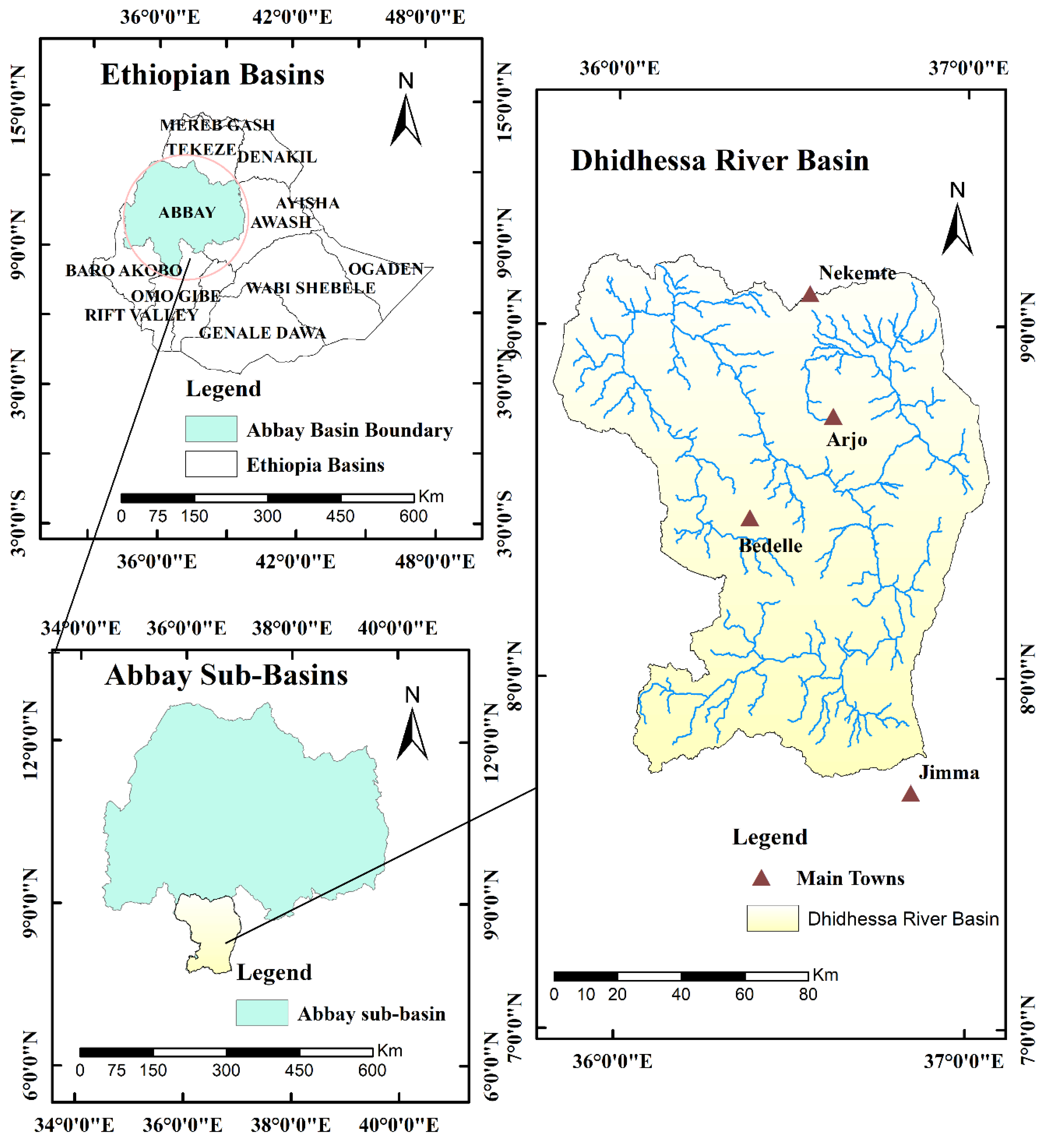
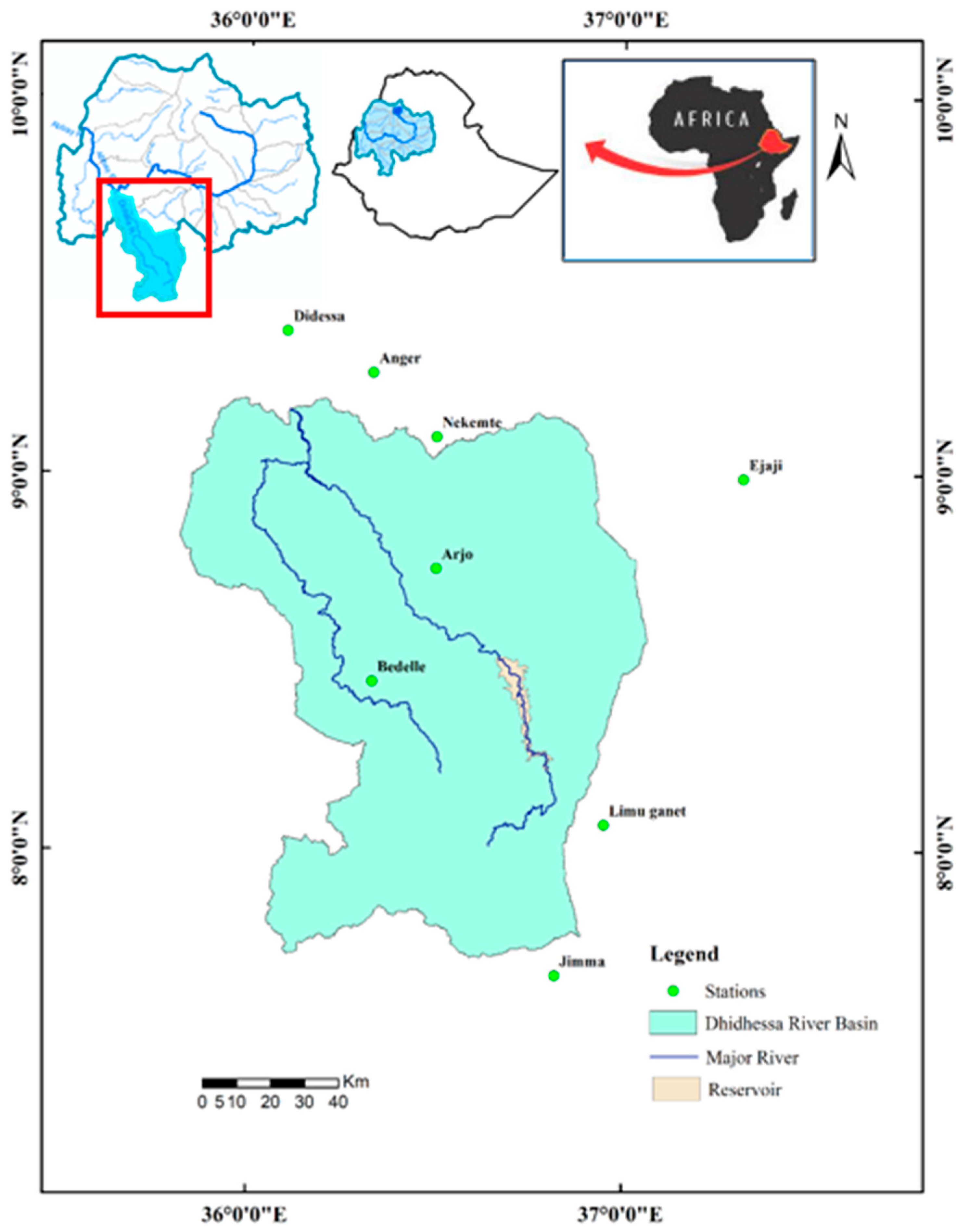
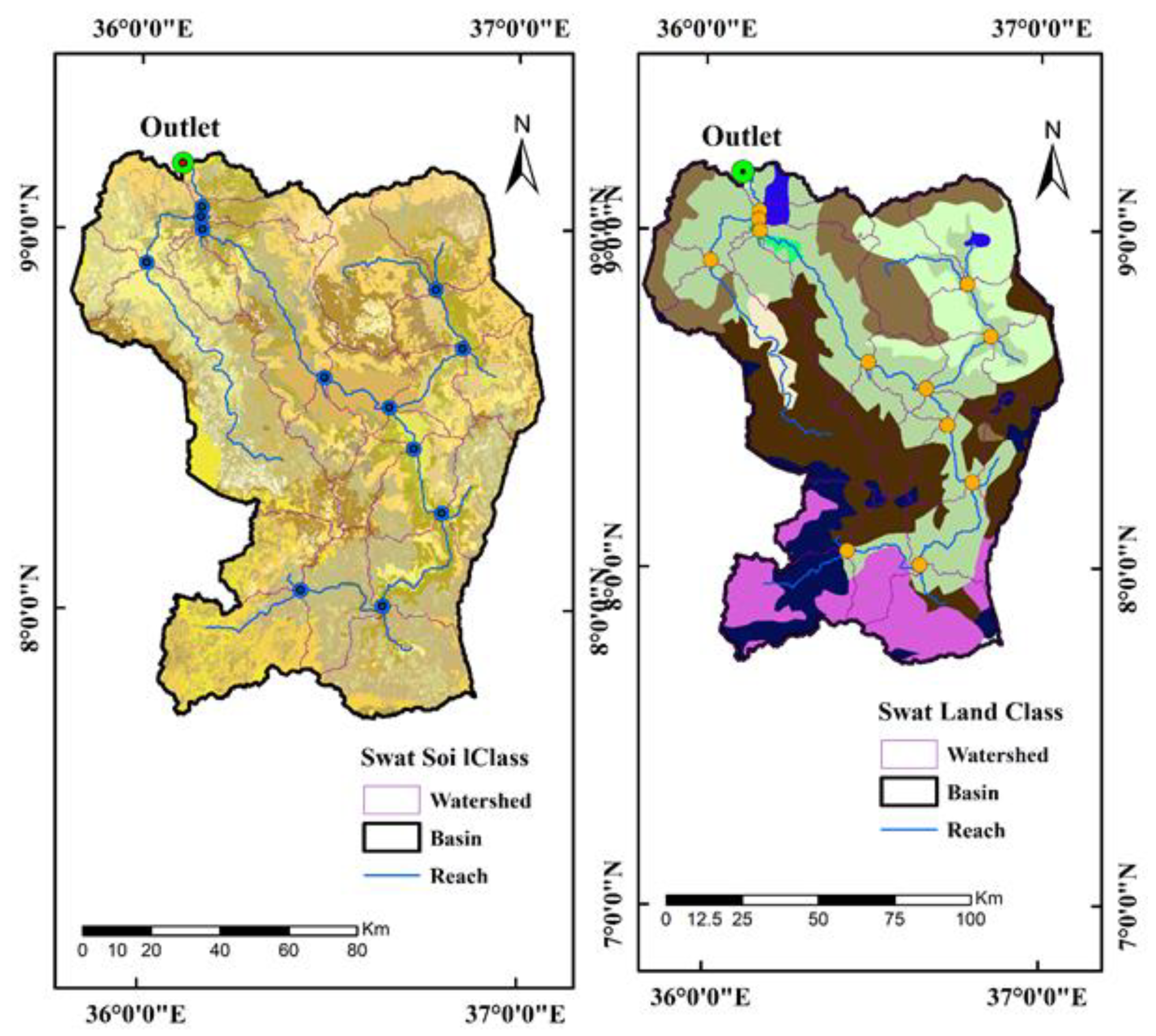
2.1. Description of the Study Area

The Dhidhessa River Basin (DRB) is located in the western part of Ethiopia between approximately 7°–9° N and 35°–36° E. The overall elevation in the study area varies between 954 and 3154 m above the mean sea level (Figure 1). The river drains about 14,710 km². Most of the DRB is classified under a humid tropical climate with heavy rainfall with an annual amount that is mainly received during the rainy season [36]. The highest and lowest temperature ranges between 21–31 °C and 10–15 °C, respectively. The mean annual flow of the DRB at the Arjo station (Figure 2) is about 341 and 318 m³/s, respectively. The river reaches its maximum flow occurring during August to September.

The basin is characterized with diversified land use/land cover that includes moderately and intensively cultivated land (50%), dense woodland (7%), wooded grassland (8%), open woodland (7%), natural forest cover (9%), natural forest with coffee (5%), coffee farm with shade trees (6%), riverine forest, bamboo forest, plantation forest, settlement (1%), shrublands and open grassland (7%). The cultivated land consists of mixed cultivation, coffee production, livestock production, subsistence and commercial forest products utilization, non-timber products utilization, beekeeping, wildlife management and utilization, infrastructure development, mining and different investment activities [60,61].

2.2. Data Collection and Processing

Daily river discharge and meteorological data (rainfall, temperature, relative humidity, sunshine hours, and wind speed) were used in this study [62,63]. Digital elevation model (DEM) of 30 × 30 m resolution was used as input for the SWAT model. Based on the DEM data, sub-basins were delineated and other essential physiographic parameters were estimated for water resources estimation. The physiographic parameters include, among others, the hydrological response units (HRUs) and the slope. Moreover, soil and land use maps were used to analyze the irrigation potential of the basin [64].

2.2.1. Climate

The daily meteorological data including daily rainfall, temperature, wind speed, sunshine hours, and relative humidity of existing stations were obtained from the Ethiopian National Meteorological Service Agency (ENMSA). These data include stations that are within and around the DRB and are classified from class 1 to 4. The definition of each class is given on the ENMSA’s official website (www.ethiomet.gov.et/). The time-series data of all stations have got continuous missing values, as indicated in the missing column in

Table 1. The list of meteorological stations in the study area.

S/n	Station Name	Elevation (m)	Data Coverage (year)	Missed (%)
1	Anger	1350	1986–2013	27.89
2	Arjo	2565	1986–2013	27.80
3	Bedelle	2011	1986–2013	1.34
4	Didessa	1310	1986–2013	28.19
5	Ejaji	1732	1986–2013	26.7
6	Jima	1718	1986–2013	0.18
7	Limu ganet	1766	1986–2013	4.28
8	Nekemte	2080	1986–2013	1.32

. The missing data can be filled automatically in the SWAT model using the weather generator. However, due to lack of completed datasets to create SWAT’s weather generator, in this study the missing climatic data were filled manually using recorded data from the nearby stations. The latter helped to appropriately check the data quality and conduct the objective of the hydrological analysis of this study. For this, eight stations that fall into class 1 were screened based on their location to the study area (Table 1). Then missing values were filled based on the recorded values in the surrounding stations. This was completed by using quality controls description and performing direct replace or rainfall contour lines to fill the rainfall gap and average methods based on data from the surrounding stations. The locations of class 1 stations are shown in Figure 2.

2.2.2. Discharge Data

The streamflow data collected at Dhidhessa near the Arjo station by the Ministry of Water, Irrigation and Energy (MoWIE) features more extended time-series data (1989 to 2012). Visually gross data errors, such as missed erroneous and noises on recorded flows were checked to ensure the data quality.

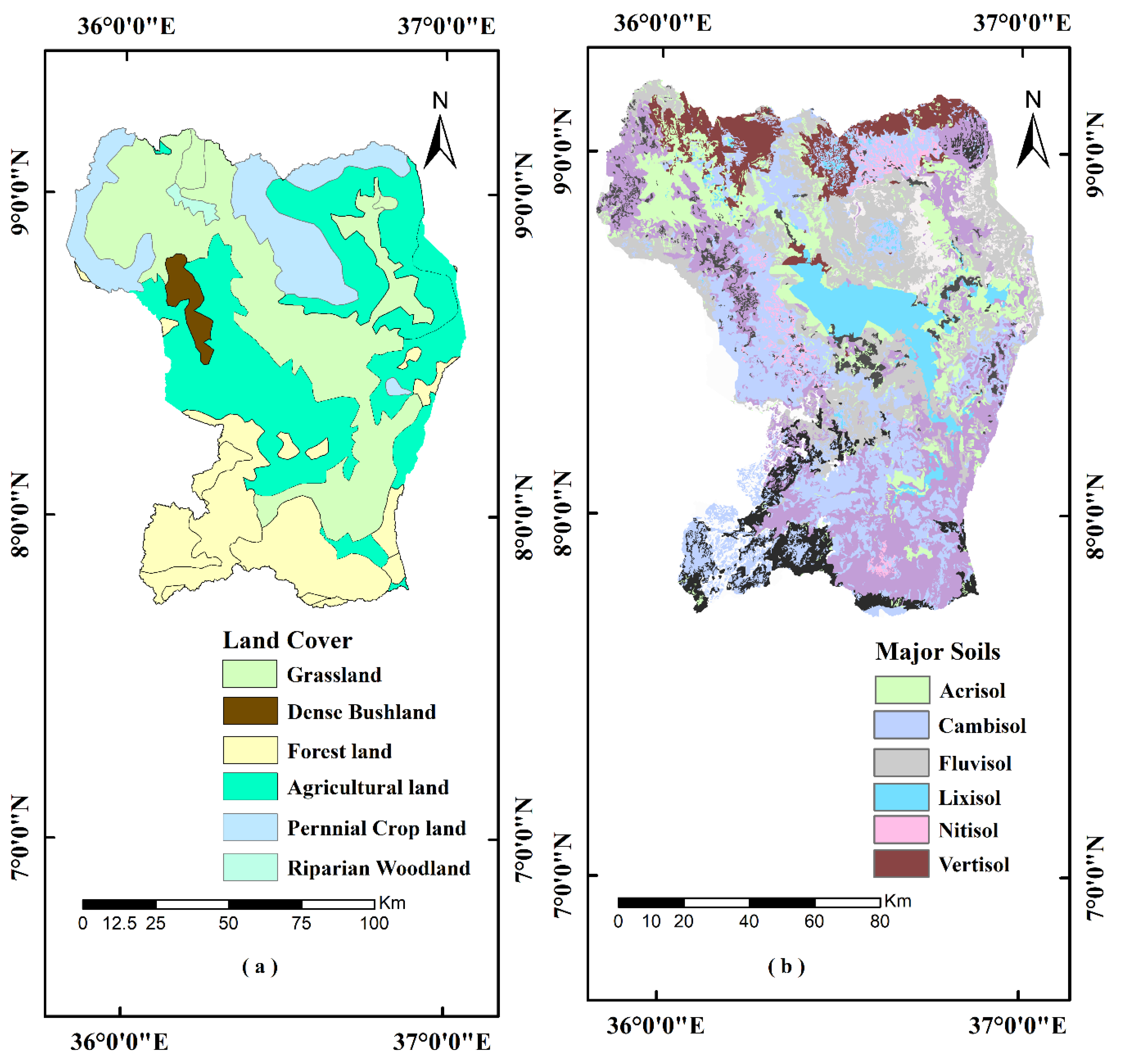
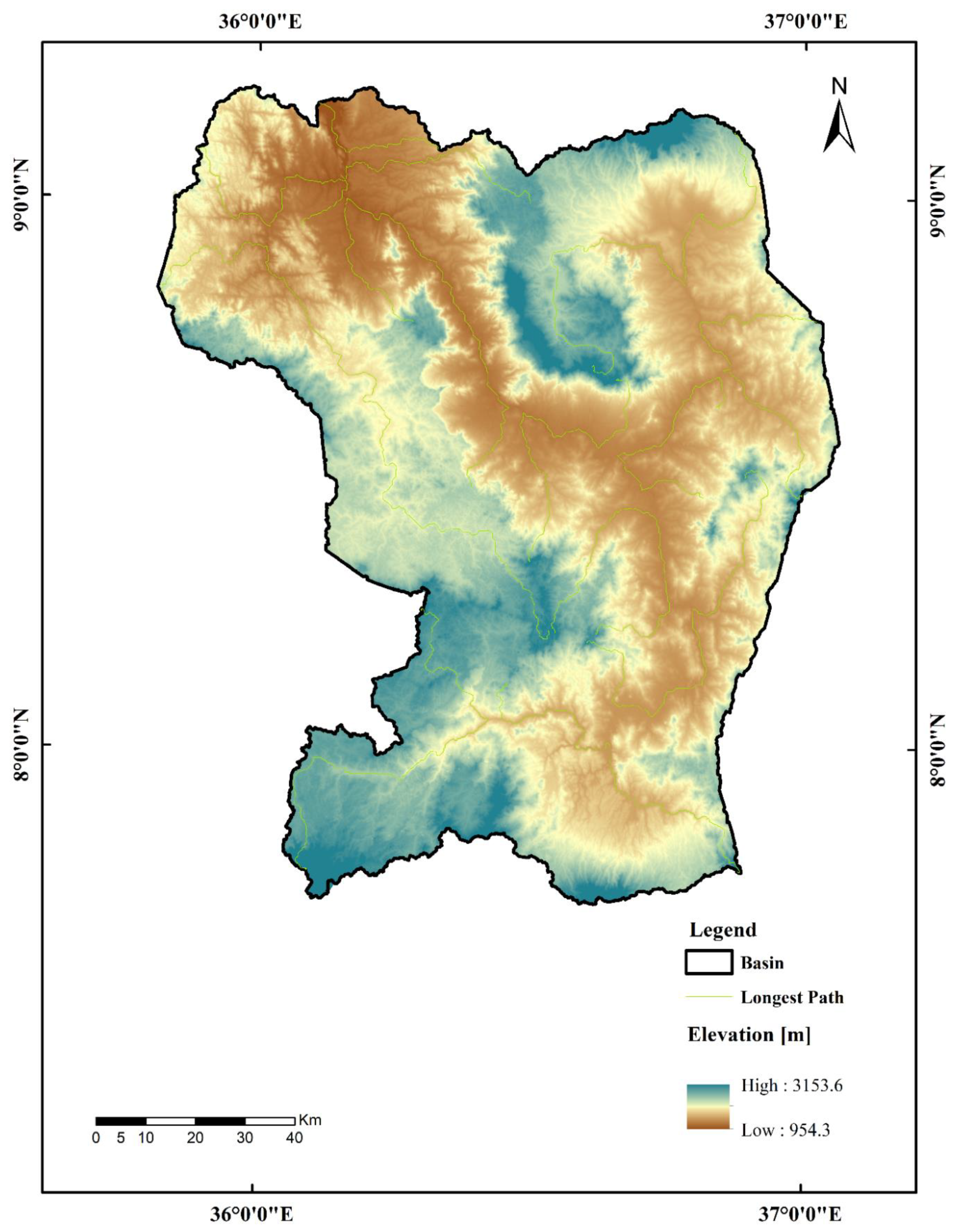
2.2.3. Physiographical Data

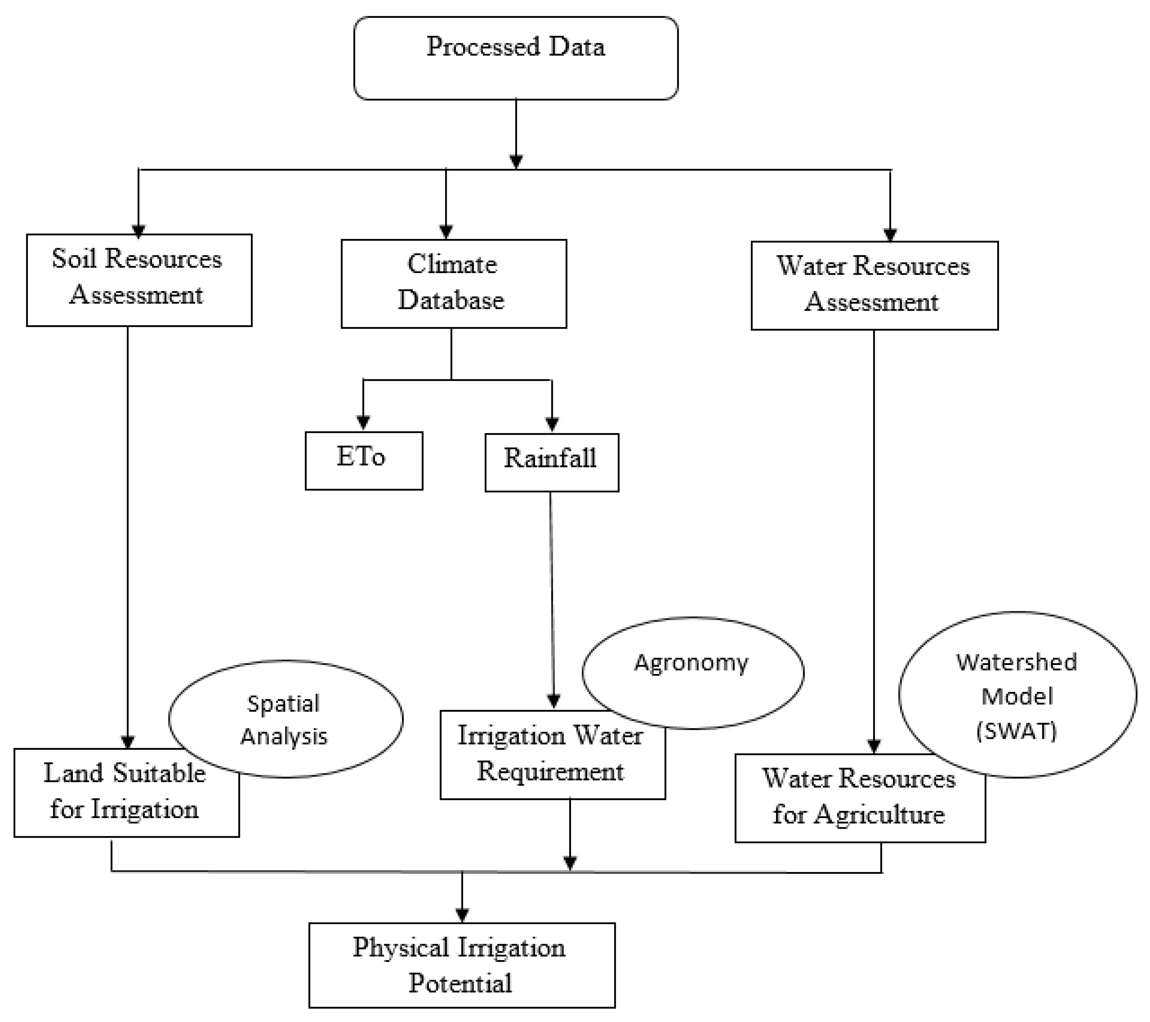
Sub-basin parameters, such as the slope gradient, and slope length, and the stream network characteristics, such as the channel slope, length, and width, were derived from the DEM data (Figure 2). The land use and soil parameters were derived from Figure 3 and used to identify potentially irrigable land and water resources. All the secondary data, such as the hydrological, meteorological and agricultural data were obtained from the Oromia Water Works Design and Supervision Enterprise (OWWDSE).

2.3. Methods

2.3.1. SWAT Model

The water availability in the DRB was simulated using the SWAT model, which is a semi-distributed, and physically based model [65]. This model has been widely used to evaluate land management practices, sediment transport, and nutrient loading and discharge at the basin scale. SWAT quantifies and characterizes the effect of land use management practices on water, agricultural nutrients, and sediment yields of the basin at different time spans [53,66,67]. In SWAT, a basin is sub-divided into sub-basins based on DEM [65]. The sub-basins are then further sub-divided into several hydrologic response units (HRUs) that represent a unique and homogeneous combination of slope, land use, and soil type within a sub-basin. SWAT computes the hydrological processes using the water balance concept and equations, applied at the HRU level of the model [65].

2.3.2. SWAT Sensitivity Analysis

The Sequential Uncertainty Fitting-II (SUFI-2) algorithm of the SWAT Calibration and Uncertainty Program (SWAT-CUP) was used for the sensitivity analysis (SA). SUFI-2 uses a One-factor-At-a-Time (OAT) global SA approach [68]. In this study, SA was only performed for discharge-related parameters (

Table 2. List of parameters used for calibration and validation.

Parameters	Description	Range
EPCO	Plant uptake compensation factor that expresses the amount of water needed to meet the plant’s uptake demand	0–1
ESCO	Soil evaporation compensation factor that directly influences the evapotranspiration losses from the watershed	0–1
CANMX	Maximum canopy storage	0–100
SOL_AWC	Available water capacity of the soil layer	0.2–0.3
PLAPS	Precipitation lapse rate	0–100
TLAPS	Temperature lapse rate	13–15
SLSOIL	Slope length for the lateral subsurface flow	0.4–0.5
SOL_DB	Density of the soil	1–1.6
CH_K	The hydraulic conductivity of the channel	0–500
CN2	The initial Soil Conservation Services (SCS) runoff curve number	0–100
SLSUBBSN	Average slope length	0.3–0.3
HRU_SLP	Average slope steepness	−0.3–0.3
OV_N	Manning’s n value for overland flow	−0.3–0.3
ALPHA_BF	The parameter that expresses the recession or the rate at which the groundwater is returned to the flow	0–1
GWQMN	The threshold depth of water in the shallow aquifer required to return the flow	0–5000
GW_DELAY	The required time for water leaving the bottom of the root zone to reach the shallow aquifer where it can contribute to lateral groundwater flow	1–500
GW_REVAP	Groundwater “revap” coefficient, which is a dimensionless coefficient controlling the rate of water movement between the root zone and the shallow aquifer	0.02–0.2
REVAPMN	Threshold depth of water in the shallow aquifer needed for “revap” or percolation to the deep aquifer to occur (mmH2O).	0–500
RCHRG_DP	Fraction of deep aquifer percolation fraction which recharges the deep aquifer	0–1

). Daily observed data were used for SA. The sensitivity of a parameter was determined based on the t-stat and p-value. The smaller the p-value and larger the absolute value of the t-stat are, the more sensitive the parameter will be, whereas a larger p-value and smaller t-stat indicate less sensitivity for a given watershed. p-values close to zero have a greater significance. Accordingly, sensitivity analysis significantly lessens the relative sensitivity of parameter identification, increases the precision of calibration, and decreases the uncertainty and time necessary for calculations.

We used the global sensitivity analysis option of the SUFI-2 algorithm, implemented in SWAT-CUP. The sensitivity of the parameters was computed to identify the most essential and sensitive parameters for the model calibration and validation processes, including uncertainty quantification [69]. The parameter sensitivity was ranked based on the t-statistics and level of significance at 5%. The 19 sensitivity parameters are presented in Table 2. All the selected parameters are considered sensitive and associated mainly with soil and groundwater, including EPCO, ESCO, CANMX, SOL_AWC, PLAPS, TLAPS, SLSOIL, SOL_DB, CH_K, CN2, SLSUBBSN, HRU_SLP, OV_N, ALPHA_BF, GWQMN, GW_DELAY, and GW_RECAP. The most sensitive parameters screened by SUFI-2 are enumerated in (Table 2).

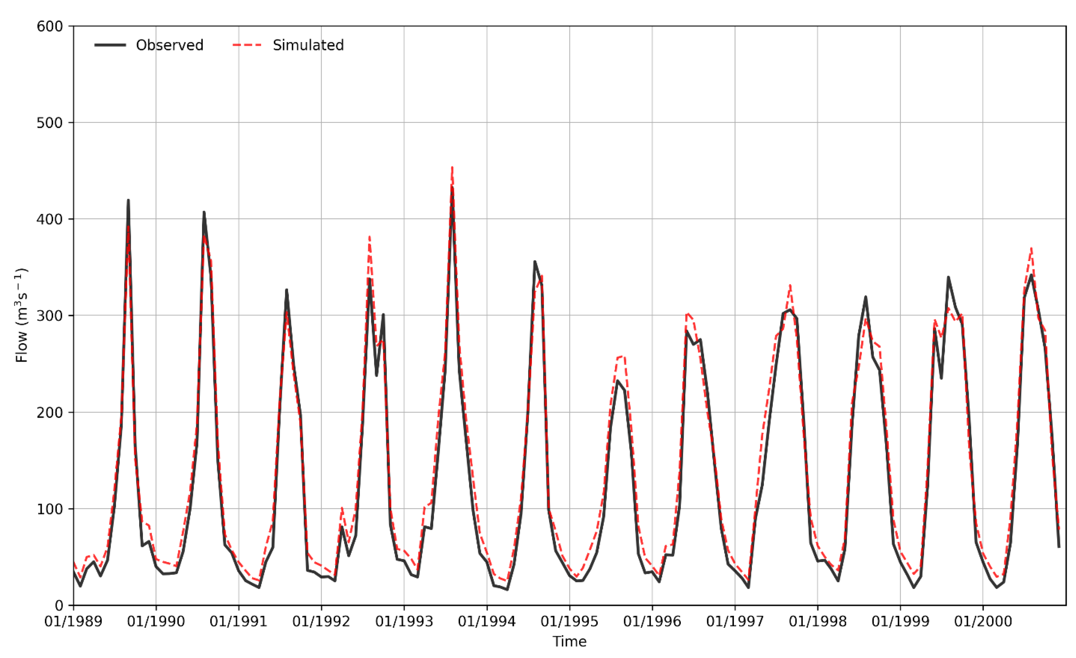
2.3.3. Model Calibration and Validation

The SWAT model was set-up for the period from 1986 to 2012. While the first three years were used for model warm up, the periods from 1989–2000 and 2001–2012 were used for model calibration and validation, respectively.

The SUFI-2 algorithm, which is included in the SWAT-CUP interface, was used to perform the SWAT model calibration and validation processes [67]. The performance of the model was evaluated by graphical comparison and using statistical indices [53,70]. The statistical criteria include the Root Mean Square Error (RMSE), Mean Absolute Error (MAE), Coefficient of determination (R²), Nash-Sutcliffe Coefficient (NSE), percent bias (PBIAS) [53,67,70]. The value of R² ranges from 0 to 1. As the value of R² approaches 1, the better is the performance of the model and values of R² that are less than 0.6 indicate poor performance of the model. The figure value of more than 0.6 is found in the satisfactory range for the coefficient of determination and a 0 value means no correlation at all; whereas 1 indicates that the desperation of the prediction is equal to that of the measured.

Additionally, we considered the model prediction uncertainty that is mapped into input model parameters. The parameter values are represented by uniform distributions. In SUFI-2, the model prediction uncertainty is quantified for the 95% prediction uncertainty (95PPU) interval. The 95PPU estimates simulated values at the 2.5% and 97.5% levels from hundreds of simulations. In this study, the 995PPU confidence interval was estimated for 500 simulations. The SUFI-2 algorithm introduces two efficiency criteria, P-factor and r-factor, that provide a measure of the model’s ability to capture uncertainties and a measure of the quality of the calibration data [65,71].

2.3.4. Model Performance Evaluation

The results of the calibration and validation were evaluated using graphical and statistical procedures based on the quality criteria [53,70]. Daily data were used for the SWAT model, where the first two years were considered as the warmup period. Then, sequential Uncertainty Fitting (SUFI-2)-based calibrations were done for a period of 12 years starting from 1989 to 2000 whereas, validation was done for the 12 years from 2001 to 2012.

The quantitative statistical parameters employed for measuring the model quality are the Root Mean Square Error (RMSE), Mean Absolute Error (MAE), Coefficient of determination (R²), Nash-Sutcliffe Coefficient (NSE), percent bias (PBIAS), p-factor, and r-factor [65,71]. The value of R² ranges from 0 to 1. The more the value of R² approaches 1, the better the performance of the model will be; conversely, values of R² less than 0.6 indicate poor performance of the model. A figure value of more than 0.6 represents a satisfactory range for the coefficient of determination, while a value of 0 means no correlation at all; conversely, 1 indicates that the determination of the prediction is equal to that of the measured value.

$$\mathrm{RMSE}=\sqrt{\frac{{{\displaystyle \sum }}_i{\left(Q_{o,i}-Q_{s,i}\right)}^2}{N}}$$

(1)

$$\mathrm{MAE}=\frac{{{\displaystyle \sum }}^{ }i\left|Q_{s,i}-Q_{o,i}\right|}{N}$$

(2)

$${\mathrm{R}}^2=\frac{{\left[{{\displaystyle \sum }}_i\left(Q_{o,i}-{\overline{Q}}_m\right)\left(Q_{s,i}-{\overline{Q}}_s\right)\right]}^2}{{{\displaystyle \sum }}_i{\left(Q_{m,i}-{\overline{Q}}_m\right)}^2{{\displaystyle \sum }}_i{\left(Q_{s,i}-{\overline{Q}}_s\right)}^2}$$

(3)

$$\mathrm{PBIAS}=\left[\frac{{{\displaystyle \sum }}_i\left(Q_{o,i}-Q_{s,i}\right)}{{{\displaystyle \sum }}_i{Q}_{o,i}}\right] \times 100$$

(4)

$$\mathrm{NSE}=1-\left[\frac{{{\displaystyle \sum }}_{i=1}^n{\left(Q_{m,i}-Q_{s,i}\right)}^2}{{{\displaystyle \sum }}_{i=1}^n{\left(Q_{m,i}-\overline{Q}\right)}^2}\right]$$

(5)

where i is the $i^{th}$ measured or simulated datum, $Q_s$ is the simulated value,$Q_m$ is the observed value, ${\overline{Q}}_m$ is the mean measured value and ${\overline{Q}}_s$ is the mean simulated value.

The Nash Sutcliffe Efficiency (NSE) was used to measure the relative magnitude of the residual variance compared to the measured data variance and define the extent of the variation between the simulated and observed data discrepancies, and its value ranges from −∞ to 1.

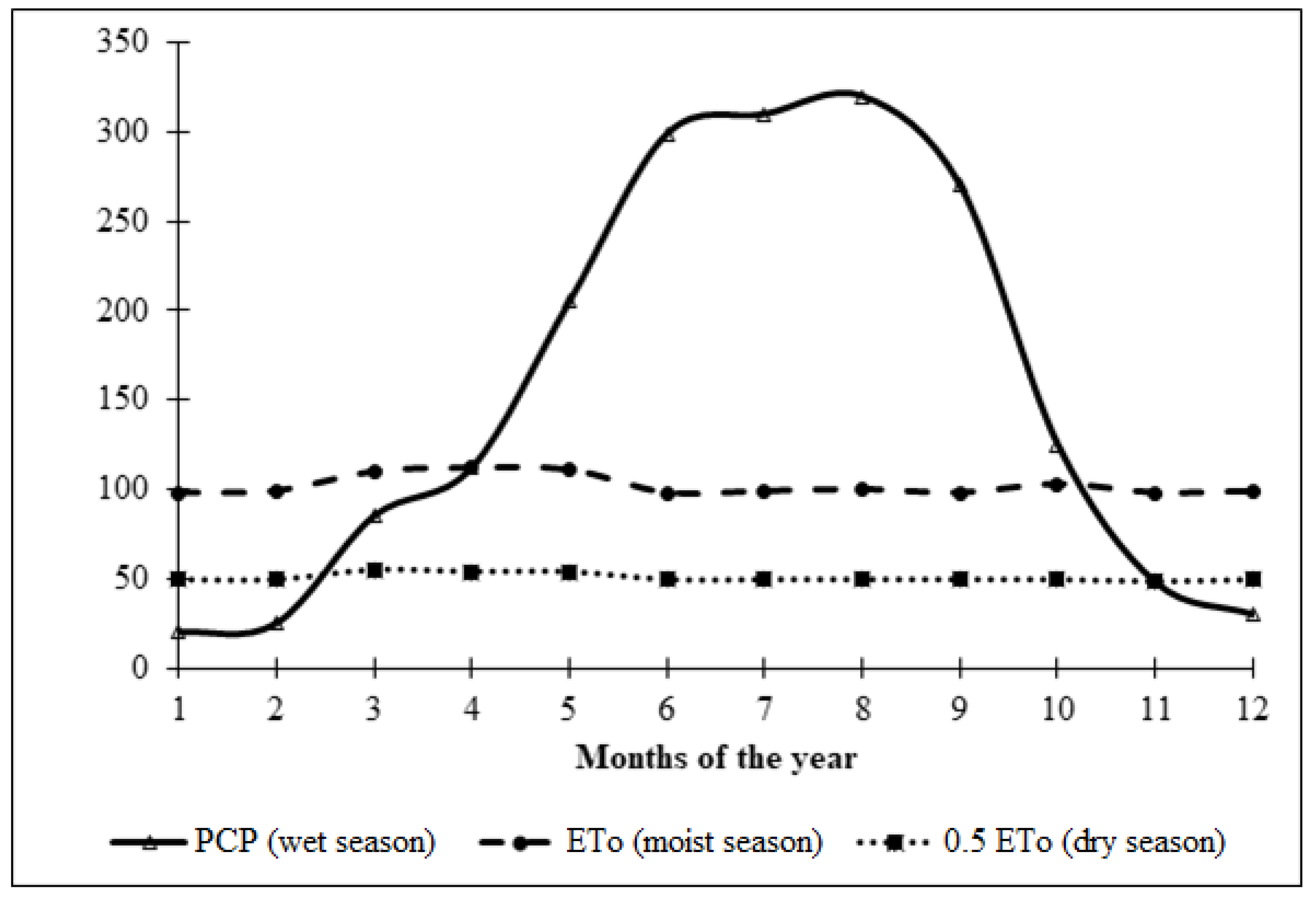
2.3.5. Assessing Water Availability

To analyze the irrigation potential of the DRB, the soil map, land use, and land cover were used as inputs for the suitability assessment. The DEM data were processed for the extraction of flow direction, flow accumulation, stream network generation and delineation of the watershed and sub-basins using ArcGIS (Figure 4). Information on low flow is required to estimate the amount of water available for surface water irrigation application during the dry season [21]. Low-flow characteristics were estimated using a flow duration curve (FDC) and by determining the 70, 80, 85 and 90-percentile available flow values. The latter is described as the flow exceedance at 70% (Q70), 80% (Q80), 85% (Q85), and 90% (Q90) of the time. A FDC at a particular outlet on a river shows the proportion of time during which the discharge at the location equals or exceeds specific values. The FDCs for long periods of runoff are useful for deciding what proportion of flow should be used for particular purposes since the area under the curve represents the volume.

The land use and soil map along with their respective lookup tables (for reclassification of according to SWAT coding conventions) were prepared as inputs for the SWAT model. The ArcGIS platform of SWAT, which referred as “ArcSWAT”, provides the user with a complete set of GIS tools for developing, running, and editing the hydrologic and management inputs of the model. The spatially distributed data required for Arc SWAT includes the Digital Elevation Model (DEM), soil and land use maps, either as shapefiles or as grid format (Figure 4 and Figure 5).

2.3.6. Computation of the Irrigation Potential Area

The irrigation potential area of the DRB was determined using the volume of water that could be supplied at varying levels of risk from the major river during the irrigation period of the selected crops (cabbage, maize, tomato, pepper, groundnut and sugarcane). Figure 6 summarizes the overall methodology used to analyze the irrigation water potential and water requirement of the upper DRB.

The gross irrigation water requirement (GIWR) is the amount of water to be extracted (by diversion or pumping) and applied to the irrigation command and scheme. The potential irrigable area was calculated as an irrigation water supply (IWS) from the river during the irrigation period divided by the GIWR. Thus, the possible irrigable area of the basin is computed based on the following.

PIA = IWS/GIWR

(6)

where PIA is the Potential Irrigable Area (ha); IWS is the Irrigation Water Supply from the river during the irrigation period (m³), and GIWR is the Gross Irrigation Water Requirement (m³/ha).

The irrigation potential area is the minimum area that can be irrigated with the available water supply (m³) divided by the annual irrigation water demand (m³/ha). This value indicates the areas that can be irrigated with the available streamflow of the sub-basin. The irrigation potential of a given sub-basin was obtained by comparing the irrigation requirements of the identified land suitable for surface irrigation system and the available mean monthly flows in the sub-basin’s river based on the suggested method [46].

To estimate the GIWR of a given crop, we used the climatic data from three different stations (Arjo, Bedelle and Angar), which represent each climatic zone of the basin. Some specific procedures recommended by the FAO for estimating missing climatic data [72,73] were applied in this study. The irrigation potential assessment mainly based on the irrigation water requirement, which was computed using the CROPWAT model depending on the cropping pattern and climate of the area [46,72,73]. The CROPWAT model was used to estimate the reference evapotranspiration (ETo) and net irrigation water requirement (NIWR). To facilitate the analysis, CROPWAT software subdivides the net irrigable area into different crop units with different planting dates at intervals of 2 to 10 days (Figure 7). The length of the growing season is the period (in days) during a year when precipitation exceeds half the evapotranspiration (i.e., PCP > 0.5 ETo). The normal growing period (also called a type three season) is characterized by a dry period, moist period (also called the intermediate period), and wet period (or also referred as the humid period).

Irrigation efficiency is a fraction of the gross irrigation water depth—that is, the net irrigation water depth needed to effectively reach the crop root zone. Irrigation water is required when rainfall is insufficient to compensate for the water lost by evapotranspiration. By calculating the soil water balance of the root zone on a daily basis, the timing and depth of future irrigations can be planned. The net irrigation water requirement was estimated using CROPWAT8. The gross irrigation water requirements at the high land, midland, and low land for different water application methods (surface, sprinkler, and drip irrigation methods) were calculated based on the net irrigation requirements.

2.3.7. Land Suitability Evaluation

This study considers the irrigation potential and offers feasible alternatives for sustainable land use and productive, without negatively impacting natural resources. To determine the irrigation potential, soil factors such as drainage, depth, texture, slope, and nutrient availability (such as pH) were evaluated. The soils in the study area have remarkable potential for a variety of rain-fed and irrigated crops. Hence the texture, depth, drainage, and pH of the soil raster, land use raster, land cover raster, and slope raster maps were generated. Moreover, a suitability model was created using the GIS model builder in the Arc tools box and the tools from the spatial analysis tool sets. Then, after individual suitability was assessed, the irrigation suitability factors considered in this study, such as the slope factor, soil factor, and land cover /use factor, were used as the input for the irrigation suitability model to determine the most suitable land for surface irrigation. The three layers (slope, soil, and land cover raster) were overlaid to find the final and suitable land.

3. Results and Discussion

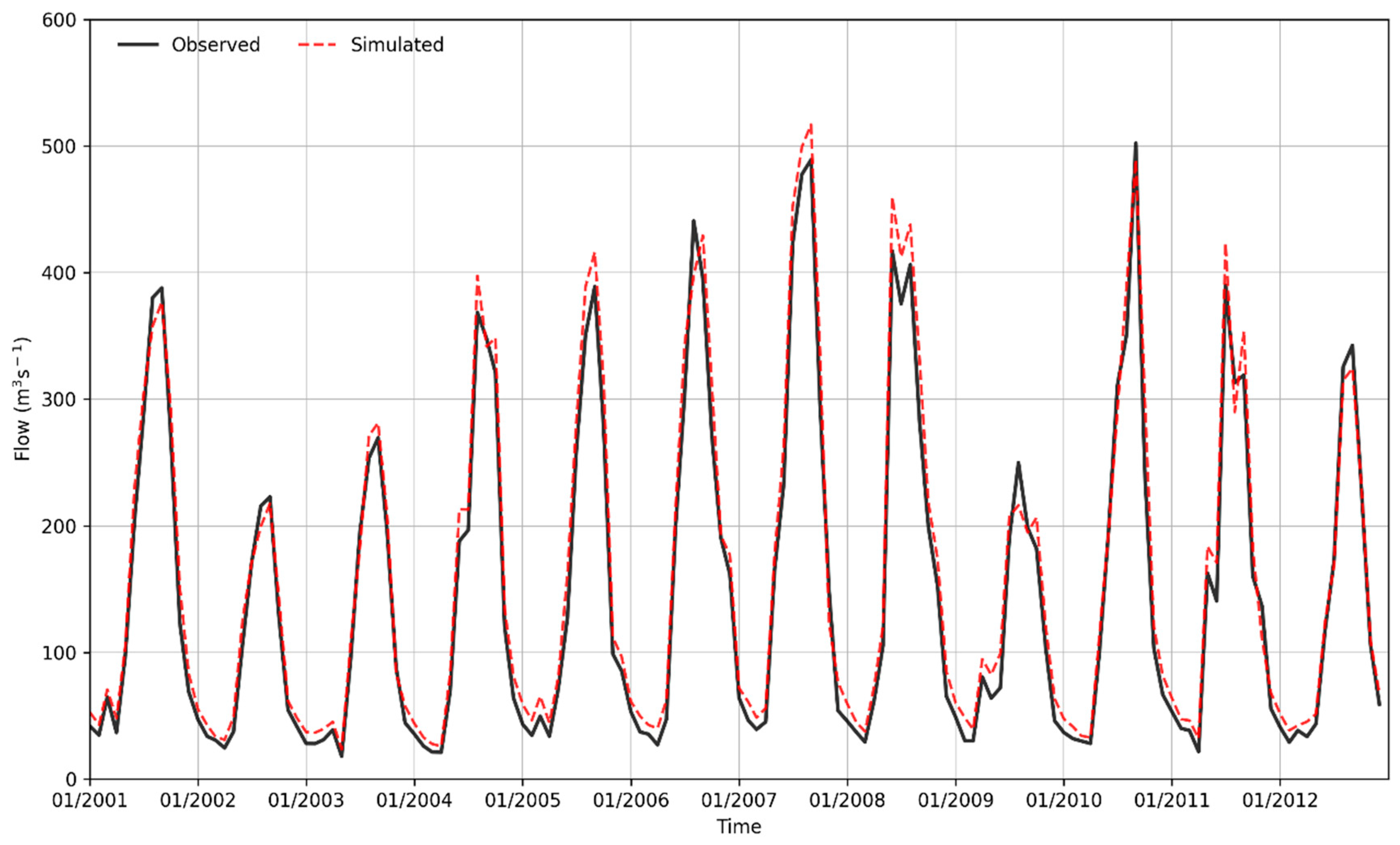
3.1. Surface Water Modelling

To assess irrigation water availability, the SWAT model was used. The sensitivity of the SWAT model parameters was determined for the flow-related parameters [69]. Before estimating the available water for irrigation, we calibrated and validated the SWAT model against observed stream flows.

Table 3. Model goodness-of-fit statistics for the calibration and validation periods.

Gaging Station	Simulation Period	Objective Function	Period	Value
Dhidhessa Near Arjo	1989–2000	R2	Calibration	0.85
		NSE		0.87
		RMSE		19.16
		MAE		16.82
		PBIAS		8.63
	2001–2012	R2	Validation	0.91
		NSE		0.89
		RMSE		19.84
		MAE		16.48
		PBIAS		8.26

NSE = Nash-Sutcliffe efficiency; R² = Coefficient of determination; RMSE = Root Mean Squared Error; MAE = Mean Absolute Error; PBIAS = Percent Bias.

summarizes the model performance using multiple statistical criteria. The values of the statistical indices of R² and NSE were 0.85 and 0.87 for the calibration period (Figure 8) and 0.91 and 0.89 for the validation period, respectively (Figure 9). These values indicate the “good” performance of the model in simulating the hydrology of the basin [53,71]. The p-factor and r- factor were 0.77 and 0.75 for the calibration period and 0.87 and 0.81 for the validation period, respectively. SUFI-2 was found to be more convenient and simpler to use compared to other automatic calibration techniques. The SWAT model performance indicates good performance that fulfills the necessary criteria [53,70]. The Dhidhessa catchment satisfies the following criteria (Table 3): The coefficient of determination is best when R² > 0.60, and the Nash–Sutcliffe (1970) coefficient of efficiency is best when NS > 0.5.

The average annual surface water potential of the upper Dhidhessa River Basin was estimated from the SWAT calibrated and validated results. It was found that the average annual precipitation and water yield of the basin are 1787 and 1605 mm of the water yield, surface water runoff contributed 146 mm, while the base flow accounts for 320 mm. Considering the basin’s area of 14,710.41 km², it was estimated that 2147 million m³ of water is delivered from the basin to the river, indicating about 9. 26 BCM is annually available for surface irrigation application.

3.2. Surface Water Availablity Assessment

To determine how much the available water can be reliably abstracted from the rivers for irrigation, flow duration analyses were carried out at a selected outlet on the river and using mean monthly simulated flow time series. The amounts of water for the different dependable flow values that can be reliably abstracted were estimated for each sub-watershed outlet.

The flows were determined by ranking all the mean monthly discharges. The purpose of the flow duration curve (FDC) analysis was to evaluate the dependable flow at various percentages for surface irrigation water use. The FDC gives the duration of occurrences in the whole range of the flow values of the river. The result indicates that the annual dependable flow values at 70% and 80% are 7.56 and 6.97 BCM, respectively (

Table 4. Result of the flow duration curve analysis under different probabilities.

Month	Jan	Feb	Mar	Apr	May	Jun	Jul	Aug	Sep	Oct	Nov	Dec
Avg. monthly (cm)	82.5	66.2	70.5	94.1	178.8	371.6	515.2	619.5	648.9	498.0	236.3	127.2
70% dependable	75.2	64.2	53.8	60.9	134.5	265.9	436.3	563.4	538.6	388.1	182.9	101.5
80% dependable	69.0	56.1	51.9	55.9	116.6	241.4	386.8	515.0	531.0	346.5	159.6	87.5
85% dependable	67.0	54.0	50.3	54.1	113.1	237.9	370.0	494.8	494.5	320.0	142.5	87.1
90% dependable	65.3	51.9	47.2	52.3	101.9	214.9	332.3	480.8	436.8	315.0	134.9	84.0

).

3.3. Potential Irrigable Area

The analyses revealed that the monthly irrigation requirements are less than the available mean monthly flow values. In addition, these mean monthly flows are slightly higher than the irrigation water requirements of the crops in their corresponding command areas.

The result of the annually available surface water in the sub-basin is 9.26 BCM. Based on the annual water supply and demand, the available water is capable of irrigating the available land suitable for agriculture. The result indicates that there is an excess amount of water resources available to satisfy the irrigation demand. Moreover, the annual irrigation potential, with respect to the physical resources and irrigation water requirements for different slope classes and dependable flow values, are shown in

Table 5. Suitable land and potential irrigable areas in different scenarios.

Slope Class	Irrigation Application Method	Agricultural Area, (ha)	For Annual Runoff	For 70% Dependable Flow	For 80% Dependable Flow
			Potential Irrigable Area, ha
less than 8%	Surface	259,028	1,104,426	901,669.8	831,301.4
	Sprinkler		1,877,267	1,532,629	1,413,019
	Drip		2,331,566	1,903,525	1,754,970
less than 15%	Surface	643,162	1,104,426	901,669.8	831,301.4
	Sprinkler		1,877,267	1,532,629	1,413,019
	Drip		2,331,566	1,903,525	1,754,970
less than 30%	Surface	1,023,581	1,104,426	901,669.8	831,301.4
	Sprinkler		1,877,267	1,532,629	1,413,019
	Drip		2,331,566	1,903,525	1,754,970

.

The irrigation potential area was estimated as the quotient of the monthly available flow and the monthly gross irrigation water requirements during the growing season of the crop. The result indicates that the potential irrigation area for the sub-basin was greater than the potentially irrigable land identified using physiographic factors for all irrigation application methods. This study also indicates that the assessed irrigation potential of the basin is higher compared to that of the Tana basin of the BNR [46].

3.4. Land Suitability Assessment Results

The land suitability shows that as the maximum slope limit increases, the suitable land area for irrigation also increases (

Table 6. Land suitable for surface irrigation with different slope scenarios.

Suitable Land When Considering a Slope of Less Than 8%
Suitability Class	Area Coverage for Different Agro-Ecological Zoning Values
	HL	LL	ML	Total
N	2630.80	557,302.41	624,851.15	1,212,012.42
S	105.88	163,014.75	95,907.77	259,028.40
% of S				17.6
Suitable Land When Considering A Slope Less Than 15%
N	2255.22	357,629.09	440,760.43	827,879.19
S	481.29	362,687.47	279,992.87	643,161.63
% of S				43.72
Suitable Land When Considering A Slope Less Than 30%
N	877.44	203,777.99	215,691.14	447,459.74
S	1859.94	516,589.64	505,131.50	1,023,581.08
% of S				69.58

N stands for non-suitable; S for suitable land; HL for highland; LL for lowland and ML for midland.

). This analysis gives useful insights into the suitable land resources development for irrigation at different slope levels. Overall, there is a large amount of land resources and potential irrigable area (1,023,581.08 ha (69.58%)) available for irrigation development and applications of the DRB.

4. Conclusions and Recommendations

In this paper, a SWAT model was developed to assess the available water resources of the Dhidhessa River Basin (DRB) for the potential application of surface water irrigation and improvement of agricultural crop productivity. The SWAT simulated flows were further analyzed using flow duration curves whereby 70% and 80% dependable flow values were estimated.

The study also estimated the irrigation water requirement of six selected crops (cabbage, maize, tomato, pepper, groundnut and sugarcane) and successfully identified their irrigation command areas. This study indicates that there is enough water to expand irrigable areas and improve the livelihoods of the local communities through implementing an enhanced irrigation system and improving agricultural crop productivity. However, improvement in irrigation efficiency depends on the choice irrigation type that plays a critical role in the water resource development and management of the Dhidhessa River. This could have an effect on satisfying the downstream environmental flow needs and water users. Therefore, to avoid more water loses in the irrigation field and to improve the irrigation water efficiency, it is highly recommended to adopt sprinkler or drip irrigation methods. This is expected to increase the irrigable area especially for command areas located in slopes ≤ 15%. This study further noticed that the identified surface irrigation potential of the DRB can assist in the decision making process and implementation of irrigation development projects in the basin. Finally, the application of remote sensing and GIS was found to be helpful in assessing the surface irrigation potential of the study area. Therefore, future irrigation development and activity would exploit these updated resources and combined with the developed SWAT model for better assessment of the land and water resources the study area and elsewhere.

References

1. Hanjra, M.A.; Qureshi, M.E. Global water crisis and future food security in an era of climate change. Food Policy 2010, 35, 365–377. [Google Scholar] [CrossRef]
2. Awulachew, S.B.; Erkossa, T.; Namara, R. Irrigation Potential in Ethiopia: Constraints and Opportunities for Enhancing the System; Unpublished Report to the Bill and Melinda Gates Foundation: Seattle, WA, USA, 2010. [Google Scholar]
3. Li, Z.; Deng, X.; Wu, F.; Hasan, S. Scenario analysis for water resources in response to land use change in the middle and upper reaches of the Heihe River Basin. Sustainability 2015, 7, 3086–3108. [Google Scholar] [CrossRef] [Green Version]
4. Watts, G.; Battarbee, R.W.; Bloomfield, J.P.; Crossman, J.; Daccache, A.; Durance, I.; Elliott, J.A.; Garner, G.; Hannaford, J.; Hannah, D.M.; et al. Climate change and water in the UK – past changes and future prospects. Prog. Phys. Geogr. 2015, 39, 6–28. [Google Scholar] [CrossRef]
5. Keshta, E.; Gad, M.A.; Amin, D. A Long–Term Response-Based Rainfall-Runoff Hydrologic Model: Case Study of The Upper Blue Nile. Hydrology 2019, 6, 69. [Google Scholar] [CrossRef] [Green Version]
6. Oki, T.; Kanae, S. Global hydrological cycles and world water resources. Science 2006, 313, 1068–1072. [Google Scholar] [CrossRef] [PubMed] [Green Version]
7. Machiwal, D.; Jha, M.K. Hydrologic Time Series Analysis: Theory and Practice; Springer Science & Business Media: New Delhi, India, 2012. [Google Scholar]
8. Olayide, O.E.; Tetteh, I.K.; Popoola, L. Differential impacts of rainfall and irrigation on agricultural production in Nigeria: Any lessons for climate-smart agriculture? Agric. Water Manag. 2016, 178, 30–36. [Google Scholar] [CrossRef] [Green Version]
9. Sanchez, P.A.; Couto, W.; Buol, S.W. The fertility capability soil classification system: Interpretation, applicability and modification. Geoderma 1982, 27, 283–309. [Google Scholar] [CrossRef]
10. Verheye, W.; Koohafkan, A.; Nachtergaele, F. The FAO guidelines for land evaluation. Encycl. Land Use Land Cover Soil Sci. Land Eval. 2009, 2, 78–100. [Google Scholar]
11. FAO; UNEP. The Future of our Land–Facing the Challenge, Guidelines for Integrated Planning for Sustainable Management of Land Resources; FAO: Rome, Italy, 1999. [Google Scholar]
12. Ayers, R.S.; Westcot, D.W. Water Quality for Agriculture; Food and Agriculture Organization of the United Nations Rome: Rome, Italy, 1985; Volume 29. [Google Scholar]
13. Huang, M.; Gallichand, J.; Wang, Z.; Goulet, M. A modification to the Soil Conservation Service curve number method for steep slopes in the Loess Plateau of China. Hydrol. Process. Int. J. 2006, 20, 579–589. [Google Scholar] [CrossRef]
14. Changnon, S.A.; Pielke, R.A., Jr.; Changnon, D.; Sylves, R.T.; Pulwarty, R. Human factors explain the increased losses from weather and climate extremes. Bull. Am. Meteorol. Soc. 2000, 81, 437–442. [Google Scholar] [CrossRef] [Green Version]
15. Easterling, D.R.; Meehl, G.A.; Parmesan, C.; Changnon, S.A.; Karl, T.R.; Mearns, L.O. Climate extremes: Observations, modeling, and impacts. Science 2000, 289, 2068–2074. [Google Scholar] [CrossRef] [Green Version]
16. Duran-Encalada, J.A.; Paucar-Caceres, A.; Bandala, E.; Wright, G. The impact of global climate change on water quantity and quality: A system dynamics approach to the US–Mexican transborder region. Eur. J. Oper. Res. 2017, 256, 567–581. [Google Scholar] [CrossRef] [Green Version]
17. Obeysekera, J.; Irizarry, M.; Park, J.; Barnes, J.; Dessalegne, T. Climate change and its implications for water resources management in south Florida. Stoch. Environ. Res. Risk Assess. 2011, 25, 495–516. [Google Scholar] [CrossRef]
18. Aswathanarayana, U. Water Resources Management and the Environment; CRC Press: Meppel, The Netherlands, 2001. [Google Scholar]
19. Taylor, R.G.; Scanlon, B.; Döll, P.; Rodell, M.; Van Beek, R.; Wada, Y.; Longuevergne, L.; Leblanc, M.; Famiglietti, J.S.; Edmunds, M. Ground water and climate change. Nat. Clim. Chang. 2013, 3, 322–329. [Google Scholar] [CrossRef] [Green Version]
20. Leta, O.T.; Bauwens, W. Assessment of the impact of climate change on daily extreme peak and low flows of Zenne basin in Belgium. Hydrology 2018, 5, 38. [Google Scholar] [CrossRef] [Green Version]
21. Worqlul, A.W.; Jeong, J.; Dile, Y.T.; Osorio, J.; Schmitter, P.; Gerik, T.; Srinivasan, R.; Clark, N. Assessing potential land suitable for surface irrigation using groundwater in Ethiopia. Appl. Geogr. 2017, 85, 1–13. [Google Scholar] [CrossRef]
22. Wang, M.; Shao, Y.; Jiang, Q.O.; Xiao, L.; Yan, H.; Gao, X.; Wang, L.; Liu, P. Impacts of Climate Change and Human Activity on the Runoff Changes in the Guishui River Basin. Land 2020, 9, 291. [Google Scholar] [CrossRef]
23. Piao, S.; Ciais, P.; Huang, Y.; Shen, Z.; Peng, S.; Li, J.; Zhou, L.; Ma, Y.; Ding, Y. The impacts of climate change on water resources and agriculture in China. Nature 2010, 467, 43–51. [Google Scholar] [CrossRef]
24. Vergine, P.; Salerno, C.; Libutti, A.; Beneduce, L.; Gatta, G.; Berardi, G.; Pollice, A. Closing the water cycle in the agro-industrial sector by reusing treated wastewater for irrigation. J. Clean. Prod. 2017, 164, 587–596. [Google Scholar] [CrossRef]
25. Rahman, M.S.; Saha, N.; Islam, A.T.; Shen, S.; Bodrud-Doza, M. Evaluation of water quality for sustainable agriculture in Bangladesh. Water Air Soil Pollut. 2017, 228, 385. [Google Scholar] [CrossRef]
26. Dinka, M.O. Quality composition and irrigation suitability of various surface water and groundwater sources at Matahara Plain. Water Resour. Res. 2016, 43, 677–689. [Google Scholar] [CrossRef]
27. Hagos, F.; Makombe, G.; Namara, R.E.; Awulachew, S.B. Importance of Irrigated Agriculture to the Ethiopian Economy: Capturing the Direct net Benefits of Irrigation, Colombo, Sri Lanka; International Water Management Institute: Anand, India, 2009; Volume 128, p. 37. [Google Scholar]
28. Lemann, T.; Roth, V.; Zeleke, G.; Subhatu, A.; Kassawmar, T.; Hurni, H. Spatial and temporal variability in hydrological responses of the Upper Blue Nile basin, Ethiopia. Water 2019, 11, 21. [Google Scholar] [CrossRef] [Green Version]
29. Araya, T.; Nyssen, J.; Govaerts, B.; Deckers, J.; Cornelis, W.M. Impacts of conservation agriculture-based farming systems on optimizing seasonal rainfall partitioning and productivity on vertisols in the Ethiopian drylands. Soil Tillage Res. 2015, 148, 1–13. [Google Scholar] [CrossRef]
30. Manaswi, C.; Thawait, A. Application of soil and water assessment tool for runoff modeling of Karam River basin in Madhya Pradesh. Int. J. Sci. Eng. Technol. 2014, 3, 529–532. [Google Scholar]
31. Fischer, G.; Tubiello, F.N.; Van Velthuizen, H.; Wiberg, D.A. Climate change impacts on irrigation water requirements: Effects of mitigation, 1990–2080. Technol. Forecast. Soc. Change 2007, 74, 1083–1107. [Google Scholar] [CrossRef] [Green Version]
32. Nelson, G.C.; Rosegrant, M.W.; Koo, J.; Robertson, R.; Sulser, T.; Zhu, T.; Ringler, C.; Msangi, S.; Palazzo, A.; Batka, M. Climate Change: Impact on Agriculture and Costs of Adaptation; International Food Policy Research Institute: Washington, DC, USA, 2009; Volume 21. [Google Scholar]
33. Farjad, B.; Pooyandeh, M.; Gupta, A.; Motamedi, M.; Marceau, D. Modelling Interactions between Land Use, Climate, and Hydrology along with Stakeholders’ Negotiation for Water Resources Management. Sustainability 2017, 9, 2022. [Google Scholar] [CrossRef] [Green Version]
34. Fiener, P.; Dlugoß, V.; Korres, W.; Schneider, K. Spatial variability of soil respiration in a small agricultural watershed—Are patterns of soil redistribution important? Catena 2012, 94, 3–16. [Google Scholar] [CrossRef]
35. Kløve, B.; Ala-Aho, P.; Bertrand, G.; Gurdak, J.J.; Kupfersberger, H.; Kværner, J.; Muotka, T.; Mykrä, H.; Preda, E.; Rossi, P.M. Climate change impacts on groundwater and dependent ecosystems. J. Hydrol. 2014, 518, 250–266. [Google Scholar] [CrossRef]
36. Gebre, S.L.; Tadele, K.; Mariam, B.G. Potential impacts of climate change on the hydrology and water resources availability of Didessa Catchment, Blue Nile River Basin, Ethiopia. J. Geol. Geosci. 2015, 4, 1–7. [Google Scholar] [CrossRef]
37. Awulachew, S.B.; McCartney, M.; Ibrahim, Y.; Shiferaw, Y.S. Evaluation of water availability and allocation in the Blue Nile Basin. In Proceedings of the 2nd International Forum on Water and Food, Addis Ababa, Ethiopia, 10–14 November 2008; p. 6. [Google Scholar]
38. Kabite, G.; Gesesse, B. Hydro-geomorphological characterization of Dhidhessa River Basin, Ethiopia. Int. Soil Water Conserv. Res. 2018, 6, 175–183. [Google Scholar] [CrossRef]
39. Adgolign, T.B.; Rao, G.V.R.S.; Abbulu, Y. Assessment of Spatio-Temporal Occurrence of Water Resources in Didissa Sub-Basin, West Ethiopia. Int. J. Civ. Struct. Environ. Infrastruct. Eng. Res. Dev. (IJCSEIERD) 2015, 5, 105–120. [Google Scholar]
40. Sima, B. Flow Regime and Land Cover Changes in the Didessa Sub-Basin of the Blue Nile River, South-Western Ethiopia. 2011. Available online:https://stud.epsilon.slu.se/2661/ (accessed on 1 July 2020).
41. MoWIE, F. Federal Democratic Republic of Ethiopia Ministry of Water, Irrigation and Electricity: Arjo Dhidhessa Dam and Appurtenant Structures Final Design Modification Report; Federal Democratic Republic of Ethiopia Ministry of Water, Irrigation and Electricity, OWWDSE/SES LLC, USA/Synergics Hydro (India) Pvt. Ltd.: Addis Ababa, Ethiopia, 2017. [Google Scholar]
42. Molden, D.J.; Awulachew, S.B.; Conniff, K.; Rebelo, L.-M.; Mohamed, Y.; Peden, D.; Kinyangi, J.; Breugel, P.V.; Mukherji, A.; Cascão, A. Nile Basin Focal Project; Synthesis Report, Project Number 59; Challenge Program on Water and Food and International Water Management Institute: Colombo, Sri Lanka, 2009. [Google Scholar]
43. Worqlul, A.W.; Ayana, E.K.; Yen, H.; Jeong, J.; MacAlister, C.; Taylor, R.; Gerik, T.J.; Steenhuis, T.S. Evaluating hydrologic responses to soil characteristics using SWAT model in a paired-watersheds in the Upper Blue Nile Basin. Catena 2018, 163, 332–341. [Google Scholar] [CrossRef]
44. Setegn, S.G.; Srinivasan, R.; Dargahi, B. Hydrological modelling in the Lake Tana Basin, Ethiopia using SWAT model. Open Hydrol. J. 2008, 2, 49–62. [Google Scholar] [CrossRef] [Green Version]
45. Zhang, L.; Xue, B.; Yan, Y.; Wang, G.; Sun, W.; Li, Z.; Yu, J.; Xie, G.; Shi, H. Model Uncertainty Analysis Methods for Semi-Arid Watersheds with Different Characteristics: A Comparative SWAT Case Study. Water 2019, 11, 1177. [Google Scholar] [CrossRef] [Green Version]
46. Worqlul, A.W.; Collick, A.S.; Rossiter, D.G.; Langan, S.; Steenhuis, T.S. Assessment of surface water irrigation potential in the Ethiopian highlands: The Lake Tana Basin. Catena 2015, 129, 76–85. [Google Scholar] [CrossRef]
47. Elliott, J.; Deryng, D.; Müller, C.; Frieler, K.; Konzmann, M.; Gerten, D.; Glotter, M.; Flörke, M.; Wada, Y.; Best, N. Constraints and potentials of future irrigation water availability on agricultural production under climate change. Proc. Natl. Acad. Sci. USA 2014, 111, 3239–3244. [Google Scholar] [CrossRef] [Green Version]
48. You, L.; Ringler, C.; Wood-Sichra, U.; Robertson, R.; Wood, S.; Zhu, T.; Nelson, G.; Guo, Z.; Sun, Y. What is the irrigation potential for Africa? A combined biophysical and socioeconomic approach. Food Policy 2011, 36, 770–782. [Google Scholar] [CrossRef] [Green Version]
49. Brauman, K.A.; Siebert, S.; Foley, J.A. Improvements in crop water productivity increase water sustainability and food security—A global analysis. Environ. Res. Lett. 2013, 8, 024030. [Google Scholar] [CrossRef]
50. Duan, Z.; Tuo, Y.; Liu, J.; Gao, H.; Song, X.; Zhang, Z.; Yang, L.; Mekonnen, D.F. Hydrological evaluation of open-access precipitation and air temperature datasets using SWAT in a poorly gauged basin in Ethiopia. J. Hydrol. 2019, 569, 612–626. [Google Scholar] [CrossRef] [Green Version]
51. Koch, M.; Cherie, N. SWAT modeling of the impact of future climate change on the hydrology and the water resources in the upper Blue Nile River basin, Ethiopia. In Proceedings of the 6th International Conference on Water Resources and Environment Research, ICWRER, Koblenz, Germany, 3–7 June 2013; pp. 488–523. [Google Scholar]
52. Van Griensven, A.; Ndomba, P.; Yalew, S.; Kilonzo, F. Critical review of SWAT applications in the upper Nile basin countries. Hydrol. Earth Syst. Sci. 2012, 16, 3371. [Google Scholar] [CrossRef] [Green Version]
53. Arnold, J.G.; Moriasi, D.N.; Gassman, P.W.; Abbaspour, K.C.; White, M.J.; Srinivasan, R.; Santhi, C.; Harmel, R.; Van Griensven, A.; Van Liew, M.W. SWAT: Model use, calibration, and validation. Trans. ASABE 2012, 55, 1491–1508. [Google Scholar] [CrossRef]
54. Alemayehu, T.; McCartney, M.; Kebede, S. The water resource implications of planned development in the Lake Tana catchment, Ethiopia. Ecohydrol. Hydrobiol. 2010, 10, 211–221. [Google Scholar] [CrossRef]
55. Belete, M.A. Modeling and Analysis of Lake Tana Sub Basin Water Resources Systems, Ethiopia; Universitat Agrar-und Umweltwissenschaftliche Fakultat: Rostock, Germany, 2014. [Google Scholar]
56. Dawit, M.; Halefom, A.; Teshome, A.; Sisay, E.; Shewayirga, B.; Dananto, M. Changes and variability of precipitation and temperature in the Guna Tana watershed, Upper Blue Nile Basin, Ethiopia. Model. Earth Syst. Environ. 2019, 5, 1395–1404. [Google Scholar] [CrossRef]
57. Setegn, S.G.; Rayner, D.; Melesse, A.M.; Dargahi, B.; Srinivasan, R. Impact of climate change on the hydroclimatology of Lake Tana Basin, Ethiopia. Water Resour. Res. 2011, 47, W04511. [Google Scholar] [CrossRef]
58. Poppe, L.; Frankl, A.; Poesen, J.; Admasu, T.; Dessie, M.; Adgo, E.; Deckers, J.; Nyssen, J. Geomorphology of the Lake Tana basin, Ethiopia. J. Maps 2013, 9, 431–437. [Google Scholar] [CrossRef] [Green Version]
59. Gadédjisso-Tossou, A.; Avellán, T.; Schütze, N. Potential of Deficit and Supplemental Irrigation under Climate Variability in Northern Togo, West Africa. Water 2018, 10, 1803. [Google Scholar] [CrossRef] [Green Version]
60. Adgolign, T.B.; Rao, G.S.; Abbulu, Y. Evaluation of Existing Environmental Protection Policies and Practices vis-à-vis Sustainable Water Resources Development in Didessa Sub-basin, West Ethiopia. Nat. Environ. Pollut. Technol. 2016, 15, 385. [Google Scholar]
61. Arnell, N.W. Climate change and global water resources. Glob. Environ. Chang. 1999, 9, S31–S49. [Google Scholar] [CrossRef]
62. Gyamfi, C.; Ndambuki, J.; Salim, R. Hydrological responses to land use/cover changes in the Olifants Basin, South Africa. Water 2016, 8, 588. [Google Scholar] [CrossRef]
63. Palazón, L.; Navas, A. Case study: Effect of climatic characterization on river discharge in an alpine-prealpine catchment of the spanish pyrenees using the SWAT model. Water 2016, 8, 471. [Google Scholar] [CrossRef]
64. Tiwari, P. Land-use changes in Himalaya and their impact on the plains ecosystem: Need for sustainable land use. Land Use Policy 2000, 17, 101–111. [Google Scholar] [CrossRef]
65. Fiseha, B.M.; Setegn, S.G.; Melesse, A.M.; Volpi, E.; Fiori, A. Hydrological analysis of the Upper Tiber River Basin, Central Italy: A watershed modelling approach. Hydrol. Process. 2013, 27, 2339–2351. [Google Scholar] [CrossRef]
66. Di Luzio, M.; Srinivasan, R.; Arnold, J.G. Integration of Watershed Tools and Swat Model into Basins 1. JAWRA J. Am. Water Resour. Assoc. 2002, 38, 1127–1141. [Google Scholar] [CrossRef]
67. Douglas-Mankin, K.; Srinivasan, R.; Arnold, J. Soil and Water Assessment Tool (SWAT) model: Current developments and applications. Trans. ASABE 2010, 53, 1423–1431. [Google Scholar] [CrossRef]
68. Abbaspour, K.C.; Yang, J.; Maximov, I.; Siber, R.; Bogner, K.; Mieleitner, J.; Zobrist, J.; Srinivasan, R. Modelling hydrology and water quality in the pre-alpine/alpine Thur watershed using SWAT. J. Hydrol. 2007, 333, 413–430. [Google Scholar] [CrossRef]
69. Mengistu, D.; Sorteberg, A. Sensitivity of SWAT simulated streamflow to climatic changes within the Eastern Nile River basin. Hydrol. Earth Syst. Sci. 2012, 16, 391. [Google Scholar] [CrossRef] [Green Version]
70. Tobin, K.J.; Bennett, M.E. Improving SWAT Model Calibration Using Soil MERGE (SMERGE). Water 2020, 12, 2039. [Google Scholar] [CrossRef]
71. Moriasi, D.N.; Gitau, M.W.; Pai, N.; Daggupati, P. Hydrologic and water quality models: Performance measures and evaluation criteria. Trans. ASABE 2015, 58, 1763–1785. [Google Scholar]
72. Melesse, A.M.; Abtew, W.; Setegn, S.G. Nile River Basin: Ecohydrological Challenges, Climate Change and Hydropolitics; Springer Science & Business Media: Geneva, Switzerland, 2014. [Google Scholar]
73. Zhou, Y.; Wenninger, J.; Yang, Z.; Yin, L.; Huang, J.; Hou, L.; Wang, X.; Zhang, D.; Uhlenbrook, S. Groundwater–surface water interactions, vegetation dependencies and implications for water resources management in the semi-arid Hailiutu River catchment, China—A synthesis. Hydrol. Earth Syst. Sci. 2013, 17, 2435. [Google Scholar] [CrossRef] [Green Version]
Figure 1. Dhidhessa sub-basin map study site, Abbay Basin, Ethiopia.
Hydrology 07 00068 g001
Figure 2. Distribution of meteorological station in and around the sub-basin.
Hydrology 07 00068 g002
Figure 3. Physiographic data (land use, land cover and major soil type).
Hydrology 07 00068 g003
Figure 4. Digital Elevation Model (DEM) of the watershed area.
Hydrology 07 00068 g004
Figure 5. Soil and land use data used in the Soil and Water Assessment Tool (SWAT) model for the Dhidhessa sub-basin.
Hydrology 07 00068 g005
Figure 6. The general flow chart for the assessment of irrigation potential. ETo: evapotranspiration.
Hydrology 07 00068 g006
Figure 7. Growing season of Arjo station within different Agro-ecological periods.
Hydrology 07 00068 g007
Figure 8. Monthly observed and simulated streamflow for the calibration period (1989–2000).
Hydrology 07 00068 g008
Figure 9. Monthly observed and simulated streamflow for the Validation period (2001–2012).
Hydrology 07 00068 g009