Analysis of the 2014 Wet Extreme in Bulgaria: Anomalies of Temperature, Precipitation and Terrestrial Water Storage

Abstract

Impact on the hydrology cycle is projected to be one of the most noticeable consequences of climate change. An increase in regional dry and wet extremes has already been observed, resulting in large socioeconomic losses. The 2014 wet conditions in Bulgaria present a valuable case study for analyzing the interaction between multiple drivers that are essential for early forecasting and warning of flood events. In this paper, time series analysis of temperature, precipitation and Terrestrial Water Storage Anomaly (TWSA) is performed and cross-correlations between observations and climate variability indices are computed for a 12-year period. In Bulgaria, a positive linear temperature trend was found with precipitation and TWSA exhibiting negative trends for the period 2003–2014. The year 2014 started with a drier and warmer than usual winter followed by five consecutive wet months from March to July. We found the following long-term variations: (1) temperature showing a local minimum in November 2014, (2) precipitation peaks in July 2014 and (3) a local TWSA maximum in December 2014. Over a 12-year period, weak to moderate negative correlations were observed between the long-term components of temperature, precipitation and TWSA. Moderate positive correlations with a 3 to 6-month lag were obtained between precipitation and TWSA long-term components. The long-term trends of temperature and precipitation from surface observations and atmospheric reanalysis showed very good alignment. Very large subseasonal precipitation residuals from observations and atmospheric reanalysis were obtained for April and September 2014. Two oscillation indices showed: (1) weak correlations with precipitation and (2) weak to moderate correlations with TWSA.

1. Introduction

Weather and climate events, driven by interacting physical processes across multiple spatial and temporal scales and leading to hazards were defined by [1] as compound events. Hazards like floods, wildfires, heat waves, and droughts are examples of compound events with multiple drivers, such as run-off, groundwater content, temperature and precipitation [1]. According to [2], there is a high probability of increasing extreme precipitation and coastal/river flood risk in Europe and, without adaptive measures, this would substantially increase flood damages. Floods are a threat not only to the safety of the population but also to national security. A MunichRE survey [3] of the number of meteorological, hydrological and climatological events that caused damage in Europe between 1980 and 2015 reported that the highest damage was caused by weather events such as convective, local, tropical and subtropical storms. According to this study, the number of extreme meteorological phenomena in Europe has increased in the last 35 years. Hydrological phenomena, such as floods and landslides, are the second most damaging natural disaster group.

Southeastern Europe has high sensitivity to extremes in the hydrology cycle, and specifically dry and wet spells. A recent example was the 2011–2012 winter, which was one of the coldest winters in decades. It was followed by an extremely hot and dry summer in 2012 with the worst drought in 40 years and wildfires. In 2014 precipitation above the norm was registered in Southeastern Europe, resulting in wide-spread floods. An extremely wet spring season was observed in the western and central Balkan peninsula. Flood casualties in May 2014 were reported in the Czech Republic, Romania, Slovakia, Croatia, Serbia and Bulgaria as well as economic loses estimated at over 1.1 billion Euro in Serbia alone. Significant precipitation between 13 and 17 May 2014, due to a stationary cyclone, lead to increased river levels, resulting in catastrophic floods. For Romania, this was the third catastrophic flood reported since late April 2014 with 125 villages and nearly 10,000 inhabitants affected. In Croatia, along the rivers Sava, Bosna and Una, tens of thousands of people were evacuated due to the floods [4]. Floods triggered about 2000 landslides on the Balkan peninsula, some of which inflicted damage to large cities and villages. As a result of muddy landslides, several rivers merged with the catchments of the Sava and Morava rivers. The water volumes of several rivers increased, leading to swampy waters inundating surrounding valleys and causing high economic losses and 49 casualties. The disaster began on 13 May 2014 when the cyclone Ivet formed and then moved from the Mediterranean to Southeastern Europe. Storing enough moisture and warm air from the Adriatic Sea, the cyclone reached the Balkan peninsula, where the air mass experienced strong orographic uplift when passing the Dinaric mountains. That led to extremely large precipitation amounts for the next 4 days. The most significant precipitation in Serbia was recorded from 14 May to 16 May in Belgrade, where for 72 h the precipitation amount reached almost 190 mm. Daily precipitation in 15 May exceeded the historic records of 107.9 mm in Belgrade, 108.2 mm in Veljevo and 110 mm in Loznitsa. On the same day in Belgrade, the 1897 monthly record of 175 mm was exceeded, and a new record of 278 mm was set [5,6]. The authors of [7] studied the climatic and meteorological factors that influence the catastrophic floods in the Balkans, focusing on large-scale circulation. They reported that the cyclone Ivet was unusually stationary, bringing extreme precipitation for several consecutive days, and linked this to a quasi-stationary Rossby wave train. In Bulgaria, according to the National Statistical Institute, in 2014 360 floods were registered, with considerable economic losses in the cities of Varna, Dobrich, Mizia, Burgas, Primorsko and Haskovo [8]. The authors of [9] analyzed the meteorologic and hydrologic conditions for 12 major flood events in 2014 in Bulgaria. They reported that four events (24–25 April, 30–31 July, 1–2 August and 23–25 October) were associated with Mediterranean cyclones approaching from the west, southwest or south. One event on 4–6 June 2014 was related to an Atlantic ocean air mass. Three events on 19 April, 15 June and 19–20 June were related to continental air masses from the north, northeast or northwest. The events on 27 January, 28–31 May, 2–7 September and 4–6 December were a result of the combined influence of Mediterranean, Atlantic, continental and polar air masses. As shown by Stoycheva et al. [9], in 2014 floods in Bulgaria started as early as January and continued until December. For example, the annual precipitation in the capital of Bulgaria, Sofia, was 168% higher than the mean of the previous 20 years.

Climate oscillation indices have a direct relation to flood occurrence through their influence on precipitation patterns. It is well known that the North Atlantic oscillation (NAO) plays an important role in the inter-annual variability of the European climate [10]. For example, the authors of [11] investigated the effect of the NAO over the Iberian Peninsula and showed that the winter NAO index was negatively correlated with rainy spells corresponding to large amounts of precipitation, in both frequency and intensity, over the west, southwest, and interior of the Iberian Peninsula. It was also negatively correlated with the winter precipitation maximum, and positively correlated with the winter maximum dry spells. This is consistent with the findings of [12], that Southern Europe flood and drought periods are controlled by the negative and positive NAO phases, respectively. Fluctuations in atmospheric circulation related to the NAO index are an important driver of climate variability over the Mediterranean region [13] as well, in particular for weather extremes, such as flood and drought. For example, the authors of [14] analyzed relationships between NAO phases and drought indices and the influence of the NAO on droughts in the entire Mediterranean region between 1901 and 2006. They found that during periods of positive NAO phase, droughts were recorded in Southern Europe (the Iberian Peninsula, Italy and the Balkans) and areas of Turkey and Northwest Africa.

Observations from the Gravity Recovery And Climate Experiment (GRACE) mission are a valuable data set of the terrestrial water storage (TWS). Terrestrial water storage is one of the main components of the hydrological cycle and by definition consists of all forms of water above and beneath the surface of the Earth. TWS variability is the sum of changes in snow, soil moisture, and ground water. Terrestrial water storage anomaly (TWSA) is a very important part of physically based model equations that represent water fluxes and storage processes. In [15], the main applications of GRACE data for groundwater monitoring on regional to global scales were reviewed. This study presented different approaches for estimating groundwater storage variations by using GRACE data along with hydrological model outputs, in situ data and other remotely sensed observations. Another use of GRACE data was presented in [16], where GRACE and reanalysis flux rate data were used to study water storage acceleration globally and locally. Regions of different size, climate conditions, and El Ni$\tilde{n}$o-Southern Oscillation (ENSO) influence were considered. The authors of [16] found a positive trend and a robust negative acceleration, that was to some extend reconstructed from reanalysis data and that was also present in non-ENSO signals. Correlation coefficients between GRACE and reanalysis fluxes time series ranging from 0.5 to above 0.9 were reported in [16]. The authors of [16] also found that dry periods leading to water storage increased and wet periods of negative storage rates may dominate long-term trends. GRACE data can also be incorporated into groundwater, hydrological and land surface models to improve the simulations of the terrestrial water cycle. The authors of [17] used 13 years of GRACE observations to assess the accuracy of four global numerical model realizations that simulated the continental branch of the global water cycle, including snow, surface and subsurface water contents. Monitoring of TWSA is of interest in Southeastern Europe, since it is an important component of the hydrological cycle and is related to compound events that are a common phenomenon in the region. The first compound event in Southeastern Europe analyzed using TWSA was the 2007 heat wave in Bulgaria. Time series analysis of TWSA, temperature, precipitation and integrated water vapor (IWV) showed both positive anomalies of temperature and IWV and negative precipitation and TWS anomalies during the 2007 heat wave [18]. It was found that the July TWSA values were strongly correlated with the end of winter precipitation means. The authors of [18] demonstrated the potential of GRACE TWS data in studying dry extremes in the hydrology cycle in Bulgaria.

The aim of this paper is to investigate the cross-correlations between the multiple drivers of the hydrology cycle in Bulgaria by using as a case study the wet extreme in 2014. In particular, the GRACE time series analysis of wet extremes is applied for the first time in Southeast Europe and its added value to the widely used temperature and precipitation time series is demonstrated. TWSA has a potential to be one of the key flood early warning indicators advancing the seasonal flood predictions in the region. In Section 2 the data sets and the analysis methods are presented. Section 3 presents the time series decomposition of temperature, precipitation and TWS, as well as cross-correlations with four climate indices for the study period of 2003–2014. In Section 3.3 we evaluate atmospheric reanalysis (ERA5) temperature and precipitation time series over the 2003–2014 period, as ERA5 is a valuable tool for regional studies. There are two reasons for this. Firstly, Southeastern Europe topography makes the modeling of the interaction between air mass and topography challenging. Secondly, precipitation is generally weakly modeled as it depends on the interaction between atmospheric dynamic and hydrologic cycle. Conclusions are presented in Section 4.

2. Data Sets and Method

In this work, surface and satellite data sets from the Sofia University Atmospheric Data Archive are used (SUADA, [19]).

2.1. Grace TWS Data

The GRACE space mission, launched in March 2002, was developed by the National Aeronautics and Space Administration (NASA) and the German Research Center for Geosciences (GFZ). It consists of two satellites placed 220 km apart on a near polar orbit with a flight altitude of 500 km at launch, which went down to 340 km in 2017. The GRACE twin satellites are connected with a highly precise K-band microwave system, which measures the change in the distance between the satellites. Variations in the distance between the satellites occur when the lead spacecraft passes above a large mass concentration that pulls it away from the second GRACE satellite trailing in the same orbital plane [20]. These measurements, along with Global Navigation Satellite Systems based location information, are used to compute dynamic satellite trajectories and monthly gravity field solutions in a common orbit and force a model parameter estimation process [21]. A GRACE follow-up mission was successfully launched in May 2018 [22] and is equipped with an innovative laser ranging interferometer to improve the measurement precision [23]. In this paper, Release-06 GRACE monthly 1${}^{\circ }$ × 1${}^{\circ }$ gridded time series of TWS, expressed in terms of equivalent water height, are used. The data are available at the international Combination Service for Time-variable Gravity Fields (COST-G [24]), which is a product center of International Gravity field Service (IGFS). We used TWSA data from three different data processing centers: (1) the Center for Space Research (CSR) at the University of Texas at Austin, (2) the German Research Center for Geosciences (GFZ) and (3) NASA’s Jet Propulsion Laboratory (JPL). In this study, time series for a single point, extracted from a 1${}^{\circ }$ × 1${}^{\circ }$ grid, were used. The extraction was done for the coordinates of Sofia, Bulgaria (longitude 23.4${}^{\circ }$ E and latitude 42.7${}^{\circ }$ N).

2.2. Surface Synoptic Data

In this study, surface synoptic observations (SYNOP) of temperature and precipitation from the Sofia station (altitude 595 m asl) were acquired from OGIMET [25] and stored in the SUADA SYNOP table. The surface temperature (T) and precipitation (P) were extracted from SUADA and monthly mean time series and anomalies were computed. First the monthly mean for each month was calculated, then the monthly means over the entire period 2003–2014 were computed and finally the anomaly was obtained by subtracting the average for the period 2003–2014 from the corresponding average of the parameters of the individual month. The observation error was ±0.1${}^{\circ }$C for temperature and ±0.5 mm for precipitation.

2.3. ERA5

ERA5 is a climate reanalysis data set covering the period of 1950 to the present that was developed within the Copernicus Climate Change Service [26]. ERA5 is computed by the European Center for Medium-Range Weather Forecasts (ECMWF). The name ERA refers to ‘ECMWF ReAnalysis’, with ERA5 being the fifth major global reanalysis produced by ECMWF after FGGE, ERA-15, ERA-40 and ERA-Interim. ERA5 was improved significantly compared to its predecessors by: (1) offering a higher horizontal resolution of 31 km and 137 vertical levels from the surface up to 0.01 hPa (around 80 km); (2) using a more recent and advanced version of the ECMWF Integrated Forecasting System model; (3) providing hourly estimates of atmospheric variables; (4) providing a consistent representation of uncertainties for these variables; (5) using more satellite observations in the data assimilation. ERA5 data are open-access and are free to download. Monthly mean surface temperature and precipitation time series were downloaded from the ERA5 reanalysis database. Three points were extracted, which were the nearest to SYNOP station Sofia (23.4${}^{\circ }$ E, 42.7${}^{\circ }$ N, 595 m asl) and their coordinates are: (1) 23.00${}^{\circ }$ E, 42.75${}^{\circ }$ N, altitude 782.3 m asl—T${}_1$ and P${}_1$, (2) 23.25${}^{\circ }$ E, 42.75${}^{\circ }$ N, altitude 8497 m asl—T${}_2$ and P${}_2$ and (3) 23.50${}^{\circ }$ E, 42.75${}^{\circ }$ N, altitude 848.9 m asl—T${}_3$ and P${}_3$.

2.4. Oscillation Indices

In this study, four oscillation indices were chosen, namely: (1) the North Atlantic Oscillation index (NAO), (2) the Mediterranean Oscillation Index (MOI), (3) the Atlantic Multidecadal Oscillation Index (AMO) and (4) the Scandinavian oscillation index (SCAND). In Figure 1 are shown the corresponding regions and surface stations used for the calculation of the oscillation indices. NAO is defined as the difference between the surface pressure measured at the Azores and Iceland stations [27]. The link between the NAO phases and the occurrence of intense cyclones has been documented in numerous studies, and according to [28] 80% of the storm days in Central Europe occur during a moderately positive NAO phase. NAO data have monthly resolution and were downloaded from [29]. MOI is defined by [30,31] represents the relation of normalized pressure between Algeria (36.4${}^{\circ }$ N, 3.1${}^{\circ }$ E), and Cairo (30.1${}^{\circ }$ N, 31.4${}^{\circ }$ E). Monthly values of the index are available for the 1948–2016 period at [32]. AMO is the main temperature index in the North Atlantic Ocean. The AMO time series cover the period from 1856 to the present and were downloaded from [33]. The index describes the relations between large-scale changes in the Atlantic Ocean, North America and Western Europe. AMO is associated with the thermohaline circulation of the ocean and is the main driver of multi-decade fluctuations during the summer months [34]. The index is applicable for periods of several decades, and therefore the 13-year period considered here is probably too short to make crucial conclusions. SCAND is related to a major circulation center over the Scandinavian Peninsula and weaker centers over Western Europe and Eastern Russia (Western Mongolia). This index is also known as Eurasia-1 [35]. Monthly SCAND values are available for the period from 1950 to the present and were downloaded from [36]. A positive phase of the SCAND index is associated with positive anomalies and blocking anticyclones over Scandinavia and Western Russia and with lower than average temperatures throughout Central Russia and over Western Europe. The SCAND index is characteristic of the precipitation in Central and Southern Europe.

2.5. Decomposition Method

Seasonal, long-term and irregular components were extracted for all studied time series by Seasonal Trend decomposition based on Loess (STL, [37]). The STL is a robust decomposition method that is used to extract the mean seasonal cycle and to separate the remaining deseasonalized signal into low and a high-frequency components. This additive decomposition is given by Equation (1), where the original signal (X${}_{ts}$) is represented as the sum of a long-term component (X${}_{long}$), a seasonal cycle (X${}_{seas}$) and the remaining subseasonal residuals (X${}_{sub}$):

$$X_{ts}=X_{long}+X_{seas}+X_{sub},where{X}_{long}=X_{lin}+X_{inter}$$

(1)

The high-frequency residuals (X${}_{sub}$) are a combination of both a real signal representing subseasonal water storage variability and the noise that is present in the GRACE data. To analyze the long-term trends, high frequency variations are removed by low pass filters (locally weighted smoothing). Then the long-term (or low-frequency) component is further divided into a linear trend (X${}_{lin}$) and anomalies with respect to this linear trend, here referred to as inter-annual variability (X${}_{inter}$) [38]. The inter-annual anomalies correspond to the nonlinear part of the long-term component. The linear trend is first estimated from the long-term component using the Theil–Sen estimator [39]. Compared to classical linear regression, using the Theil–Sen slope provides an estimate of the trend that is more robust and less sensitive to large anomalies occurring near the beginning or end of the time series. The nonparametric Wilcoxon test is used to obtain the significance of the linear trends [40]. The null hypothesis can be rejected and linear trends are considered statistically significant as the p value falls below a critical value (p < 0.05). In addition, the cross-correlations between the decomposed components of temperature, precipitation and TWSA will be computed (at a 5% significance level) and discussed.

3. 2014 Wet Extreme in Bulgaria: Time Series Analysis

In this section the results from time series analysis of observed anomalies of temperature, precipitation and TWS during the period of 2003–2014 are reported. Furthermore, a comparison between SYNOP and ERA5 time series of temperature and precipitation is carried out. In addition, the cross-correlations between temperature, precipitation and TWSA and the oscillation indices NAO, MOI, AMO and SCAND are computed and discussed.

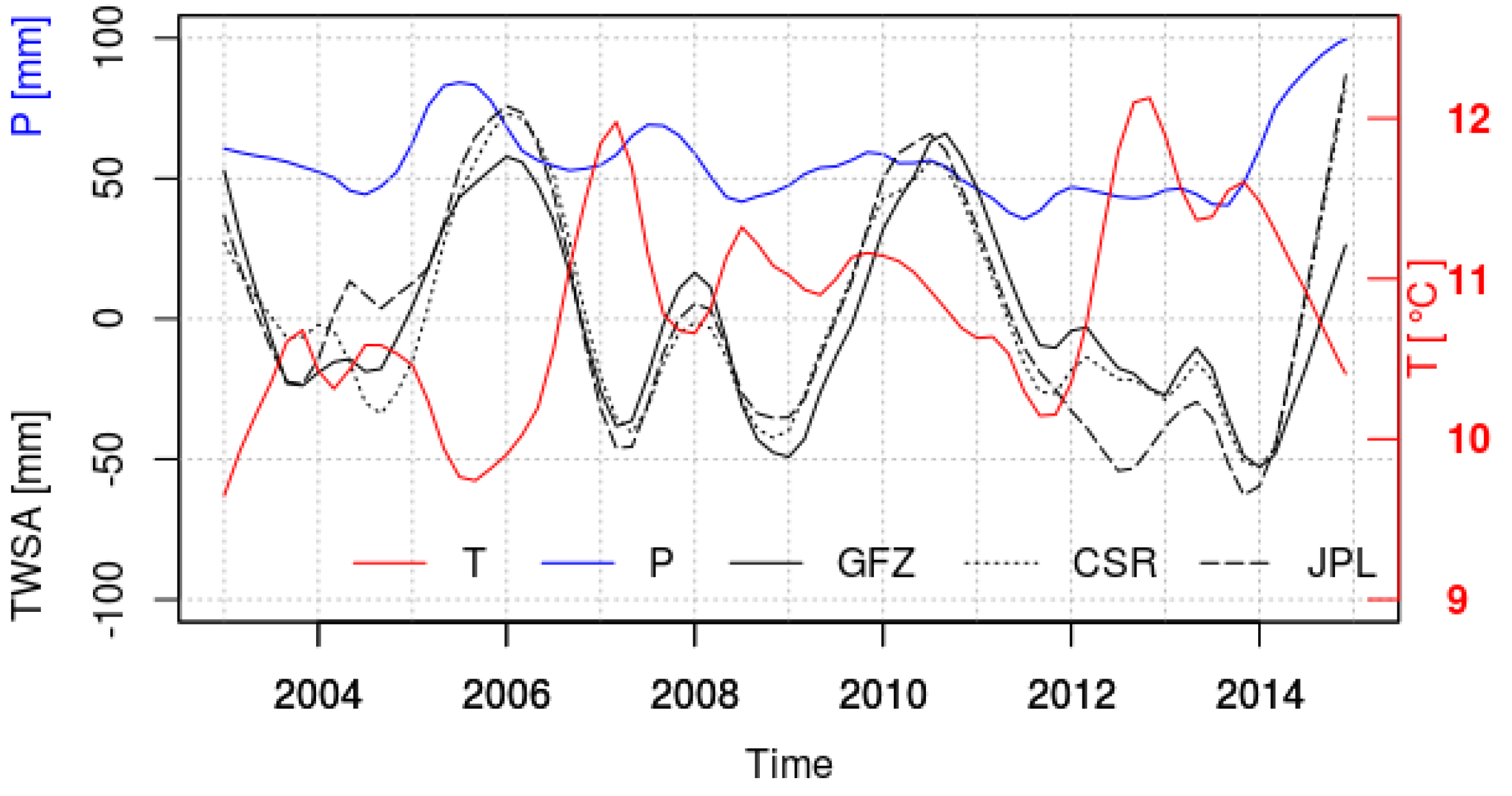
3.1. Anomalies of Temperature, Precipitation and TWS in 2014

Monthly mean temperature and precipitation anomalies in Sofia for 2014 are plotted in Figure 2. As seen from Figure 2a, large positive temperature anomalies in January (1.5 ${}^{\circ }$C), February (4.4 ${}^{\circ }$C) and March (2.3 ${}^{\circ }$C) were followed by negative anomalies from May to July 2014. The largest negative anomalies were in May (−1.3 ${}^{\circ }$C) and July (−1.2 ${}^{\circ }$C). It is to be noted that the July 2014 and July 2006 both had the largest negative temperature anomalies (−1.2 ${}^{\circ }$C). By contrast, the July 2012 and July 2007 temperature anomalies of 3.3 ${}^{\circ }$C and 2.2 ${}^{\circ }$C, respectively, were the largest positive anomalies and were associated with heat waves in Southeastern Europe. The 2014 precipitation monthly anomalies were mainly positive from March to September (Figure 2b). For 2014, three of the months exhibited the largest positive precipitation anomalies for the corresponding months over the 2003–2014 period: September (134 mm, 209% of the monthly mean), April (104 mm, 200% of the monthly mean) and July (104 mm, 114% of the monthly mean). For 2014, significant positive precipitation anomalies were also observed in March, May and June. In 2014, negative precipitation anomalies were observed in January and February, which in combination with positive temperature anomalies for the same months were an indication for a dry and warm start of 2014 followed by five consecutive wet months from March to July and then an even wetter September.

Figure 3 shows the monthly mean TWSA for 2014 (black line) and its variability range for the 12-year period for processing centers CSR (Figure 3a), GFZ (Figure 3b) and JPL (Figure 3c). The TWSA exhibited an annual cycle with predominantly: (1) higher than average values in the first half of the year (from January to June) and (2) lower than average values in the second half (from July to December). Comparing Figure 2b and Figure 3 it can be concluded that the TWSA maxima followed the precipitation peaks. For example, the precipitation peak in April 2014 (Figure 2b) was followed by a TWSA peak in May 2014. During the 2014 flood months, May, June and July, with six major flood events (half of all 2014 major events as reported by [9]), there was a combination of negative temperature anomalies and positive precipitation and TWS anomalies. The negative TWSA in January 2014 was the largest January anomaly over the studied period, with −92 mm, −112 mm and −116 mm for CSR, GFZ and JPL, respectively.

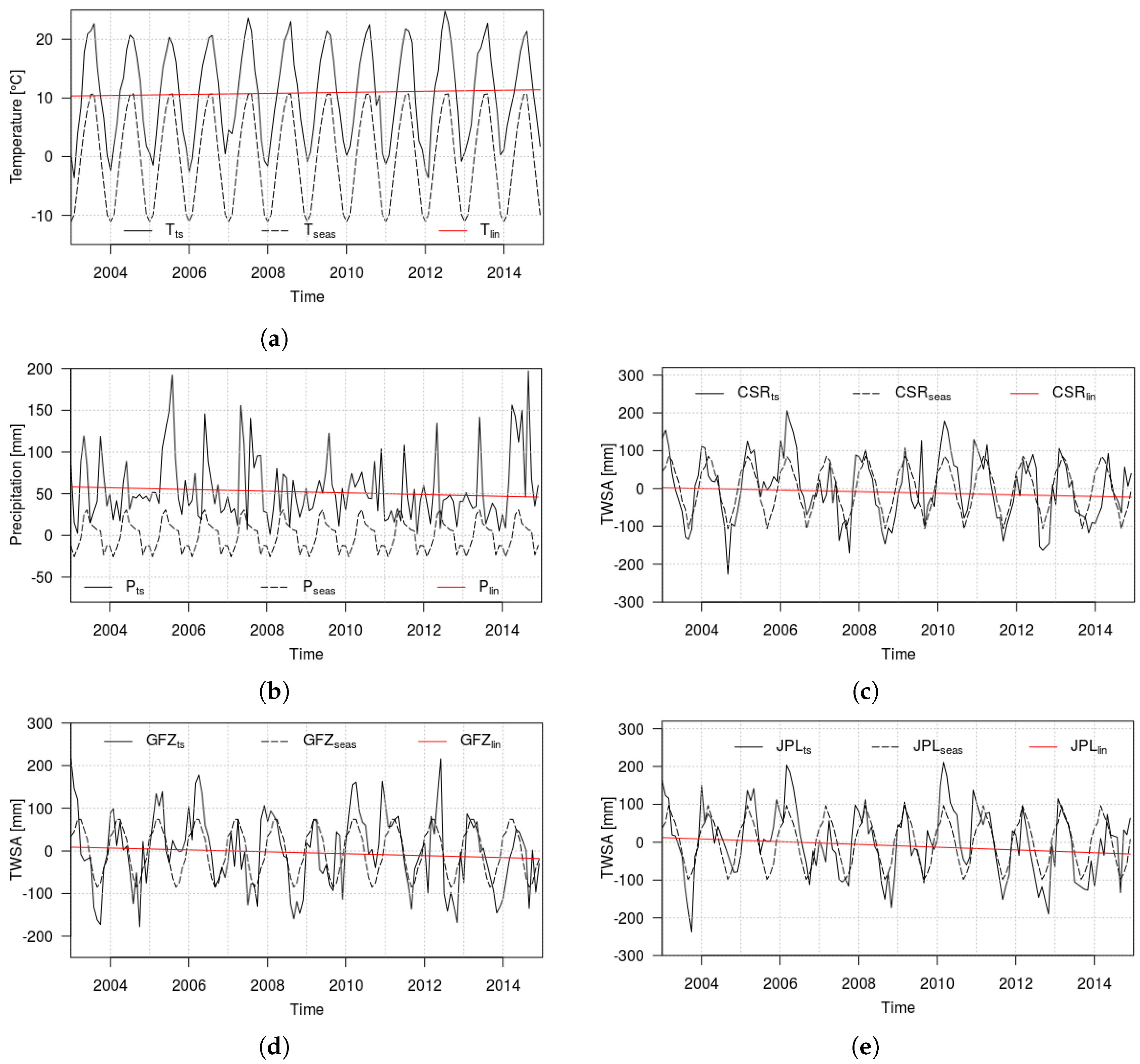
3.2. Time Series Decomposition: Temperature, Precipitation and TWSA

Figure 4, Figure 5 and Figure 6 illustrate the time series decomposition of temperature, precipitation and TWSA into high-frequency and low-frequency components by the method of seasonal trend decomposition using Loess.

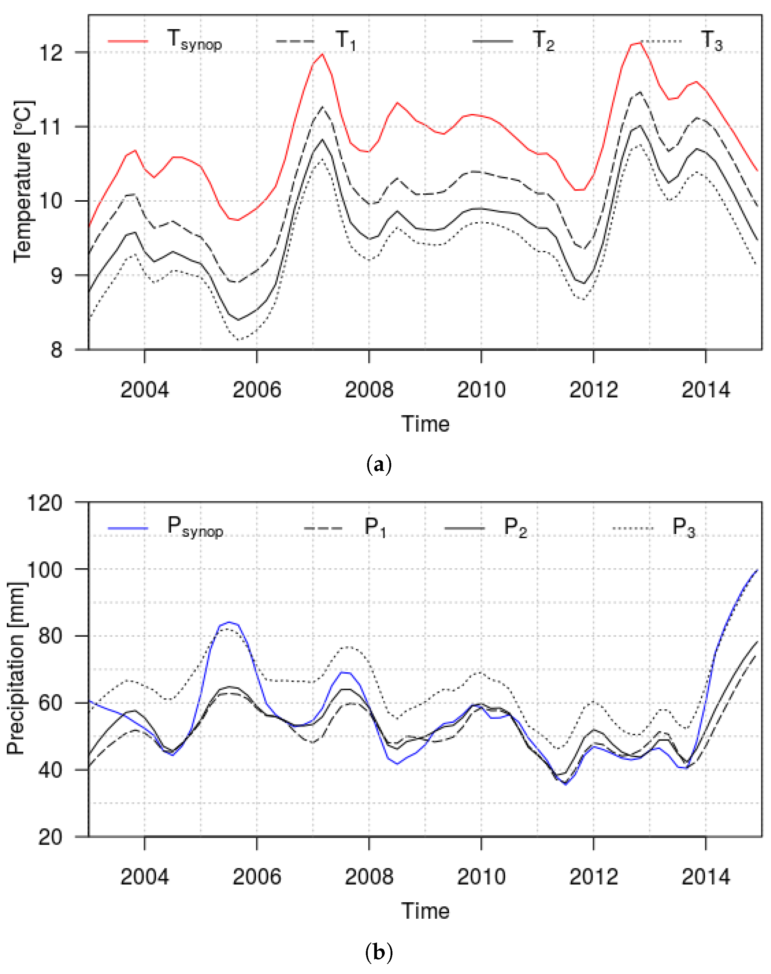
3.2.1. Long-Term Trends and Variability

In Figure 4 the long-term components of temperature, precipitation and TWSA for the 12-year period are shown. It can be seen that a negative temperature trend combined with a positive precipitation and TWSA trends for 2014. By contrast, there was a positive temperature trend and negative precipitation and TWSA trends during the summer 2007 heat wave in Bulgaria [18].

The cross-correlations between the long-term components of temperature, precipitation and TWSA for the 2003–2014 period are shown in

Table 1. Cross-correlation coefficients between the long-term trends of studied parameters over the period 2003–2014. Only values that are significant at the 5% significance level are presented. NS is for Not Significant cross-correlation.

Data	Lags in Month
	−6	−5	−4	−3	−2	−1	0	1	2	3	4	5	6
T∼P	NS	NS	NS	−0.11	−0.19	−0.26	−0.33	−0.36	−0.38	−0.40	−0.39	−0.38	−0.36
T∼ CSR${}_{twsa}$	−0.37	−0.42	−0.46	−0.50	−0.52	−0.53	−0.53	−0.48	−0.42	−0.36	−0.30	NS	NS
T∼ GFZ${}_{twsa}$	−0.34	−0.40	−0.46	−0.51	−0.55	−0.57	−0.58	−0.54	−0.50	−0.43	−0.37	−0.30	−025
T∼ JPL${}_{twsa}$	−0.33	−0.40	−0.46	−0.52	−0.57	−0.61	−0.63	−0.61	−0.57	−0.53	−0.48	−0.43	−0.37
P∼ CSR${}_{twsa}$	0.62	0.64	0.65	0.63	0.59	0.54	0.46	0.32	0.19	NS	NS	−0.15	−0.22
P∼ GFZ${}_{twsa}$	0.49	0.50	0.50	0.49	0.46	0.41	0.35	0.27	NS	NS	NS	−0.23	−0.29
P∼ JPL${}_{twsa}$	0.60	0.62	0.62	0.61	0.58	0.53	0.47	0.35	0.24	0.13	NS	NS	NS

. To assess the significance of the results we applied a test of association using Kendall’s tau [41]. In this table only significant cross-correlation coefficients at the 5% significance level are presented. Long-term components of temperature show weak to moderate negative correlations with long-term components of precipitation and TWSA. This means that there was a weak to moderate tendency for positive temperature trends to be accompanied by negative precipitation and TWSA trends. Precipitation and TWSA were moderately correlated. From Table 1 it can be seen that the highest correlations were observed with a 3 to 6-month lag. The highest cross-correlations between the long-term components of precipitation and TWSA from the different processing centers were: (1) 0.65 for CSR, (2) 0.50 for GFZ and (3) 0.62 for JPL. The observed correlations suggested that it is likely that periods with increasing/decreasing precipitation amounts will be followed 3 to 6 months later by increasing/decreasing TWSA trends.

Next, the long-term variations (X${}_{long}$) were partitioned into linear (X${}_{lin}$) and nonlinear components (X${}_{inter}$). A linear component gives information about the direction of the trend over the studied period, i.e., whether the trend is positive or negative. In Figure 5 the linear components of temperature, precipitation and TWSA are plotted. The results showed: (91) a positive temperature trend, increasing by 1.1 ${}^{\circ }$C over the 12-year period (Figure 5a) and (2) a negative precipitation trend, decreasing by 12 mm over the 12-year period (Figure 5b). TWSA time series also exhibited negative linear trends over the 12-year period, with: (1) 26 mm for CSR data and GFZ data (Figure 5c,d) and (2) 44 mm for JPL data (Figure 5e) over the 12-year period.

Inter-annual anomalies corresponded to the low-frequency and non-linear components of the signal. To get more specific information about the inter-annual anomalies, cross-correlations between temperature, TWSA and precipitation inter-annual components are analyzed. The results are shown in

Table 2. Cross-correlation coefficients between the inter-annual components of the long-term trends of studied parameters over the period 2003–2014. Only values which are significant at the 5% significance level are presented.

Data	Lags in Month
	−6	−5	−4	−3	−2	−1	0	1	2	3	4	5	6
T∼P	0.11	NS	NS	NS	NS	NS	−0.34	−0.37	−0.37	−0.37	−0.34	−0.31	−0.27
T∼ CSR${}_{twsa}$	−0.33	−0.39	−0.44	−0.49	−0.52	−0.53	−0.52	−0.45	−0.37	−0.28	NS	NS	NS
T∼ GFZ${}_{twsa}$	−0.28	−0.36	−0.43	−0.49	−0.53	−0.55	−0.56	−0.51	−0.44	−0.37	−0.30	NS	NS
T∼ JPL${}_{twsa}$	−0.21	−0.29	−0.38	−0.45	−0.52	−0.56	−0.59	−0.55	−0.50	−0.43	−0.37	−0.30	NS
P∼ CSR${}_{twsa}$	0.57	0.60	0.62	0.61	0.58	0.53	0.46	0.31	0.17	NS	NS	−0.23	−0.25
P∼ GFZ${}_{twsa}$	0.44	0.46	0.47	0.44	0.39	0.33	0.26	NS	NS	NS	NS	−0.25	−0.31
P∼ JPL${}_{twsa}$	0.53	0.56	0.58	0.58	0.56	0.52	0.48	0.35	0.23	NS	NS	NS	NS

and are summarized as follows: (1) weak to moderate negative correlations existed between temperature and precipitation inter-annual components, (2) moderate negative correlations existed between temperature and TWSA inter-annual components and (3) moderate positive correlations existed between precipitation and TWSA inter-annual components. As can be expected, temperature had a negative effect on TWSA while precipitation had a positive effect on TWSA.

3.2.2. Seasonal Cycle Component

Previous studies have shown that there is a temporal lag between the seasonal cycle component of precipitation and terrestrial water storage ([42,43,44]). The time span between TWS and precipitation seasonal maximum and minimum is about 6 months [18] in Bulgaria. In Figure 5 the seasonal components of temperature, precipitation and TWSA are plotted. Precipitation maxima were observed for the end of the spring season and beginning of the summer season (May and June), while precipitation minima were observed in the late autumn and all winter months (from November to February, Figure 5b). The TWSA maxima (Figure 5c–e) occured in spring (March and April), while the TWSA minima occured in autumn (September and October). The seasonal cycle of the temperature (Figure 5a) peaked in summer, 2 or 3 months earlier than the autumn minimum of the TWSA. The seasonal minimum of the temperature preceded by 2 or 3 months the spring maximum in the TWSA. The temperature seasonal cycle was generally out of phase with respect to the TWSA seasonal cycle.

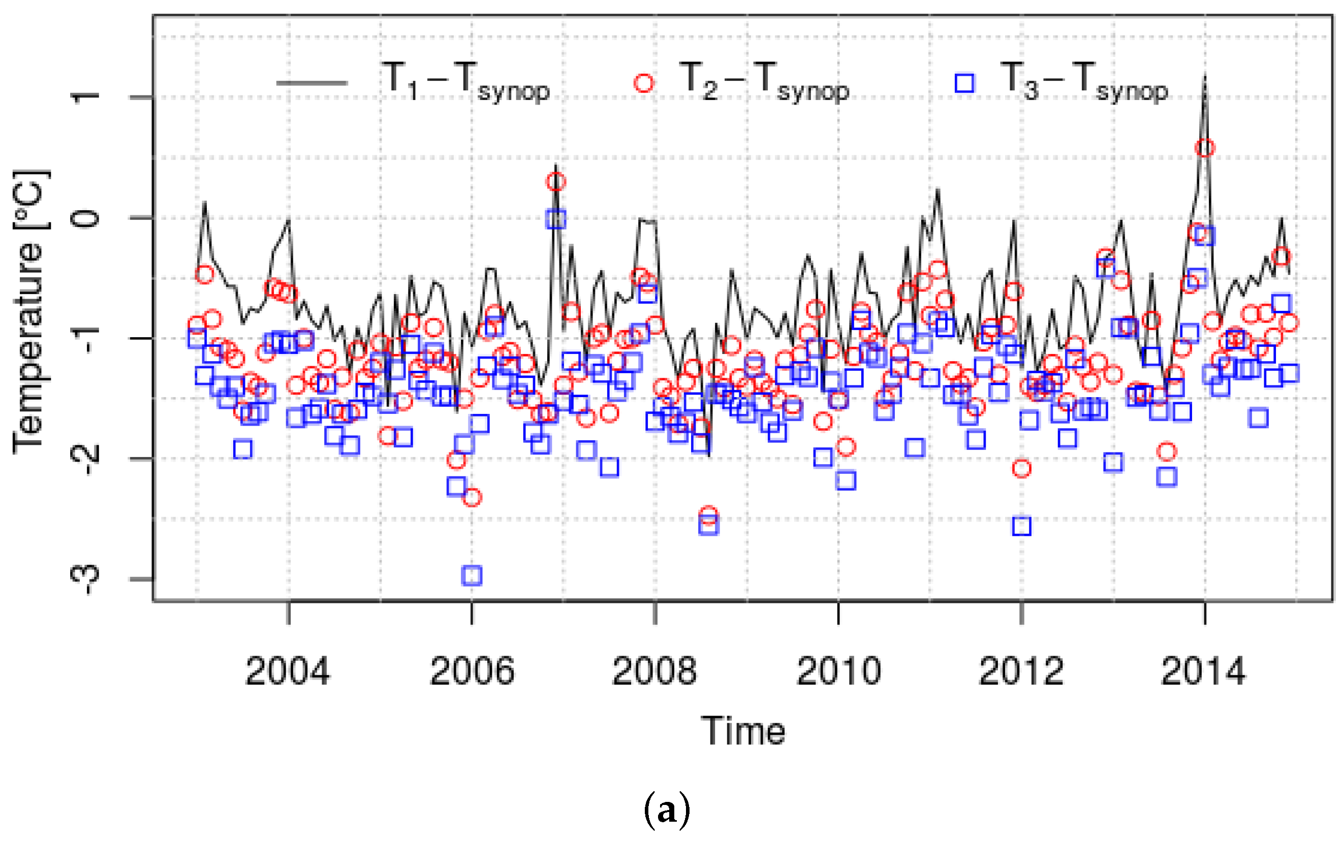
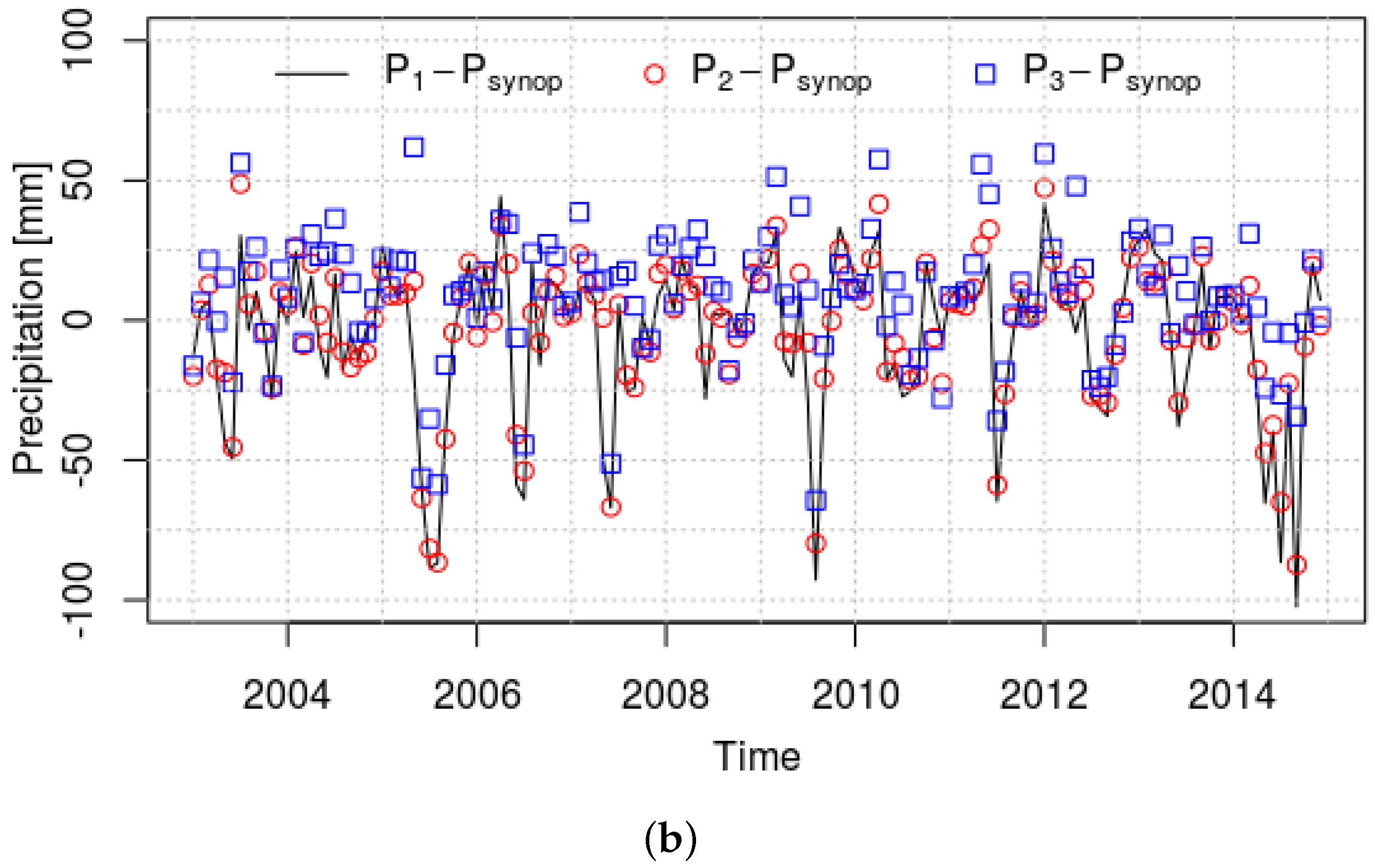
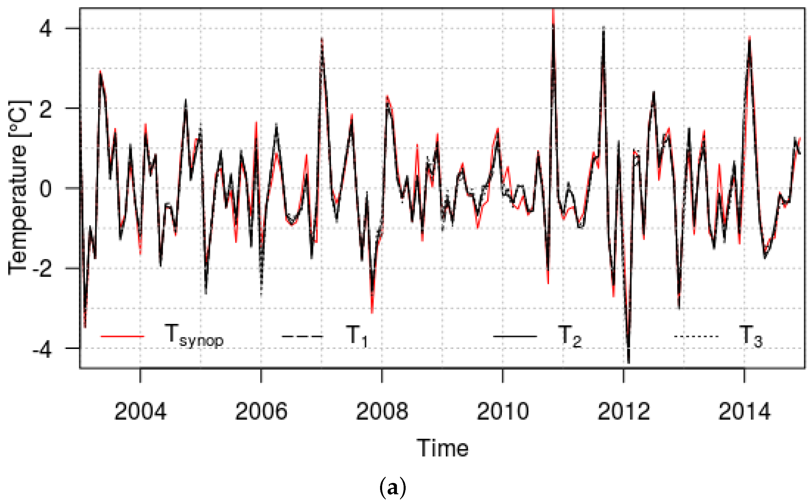
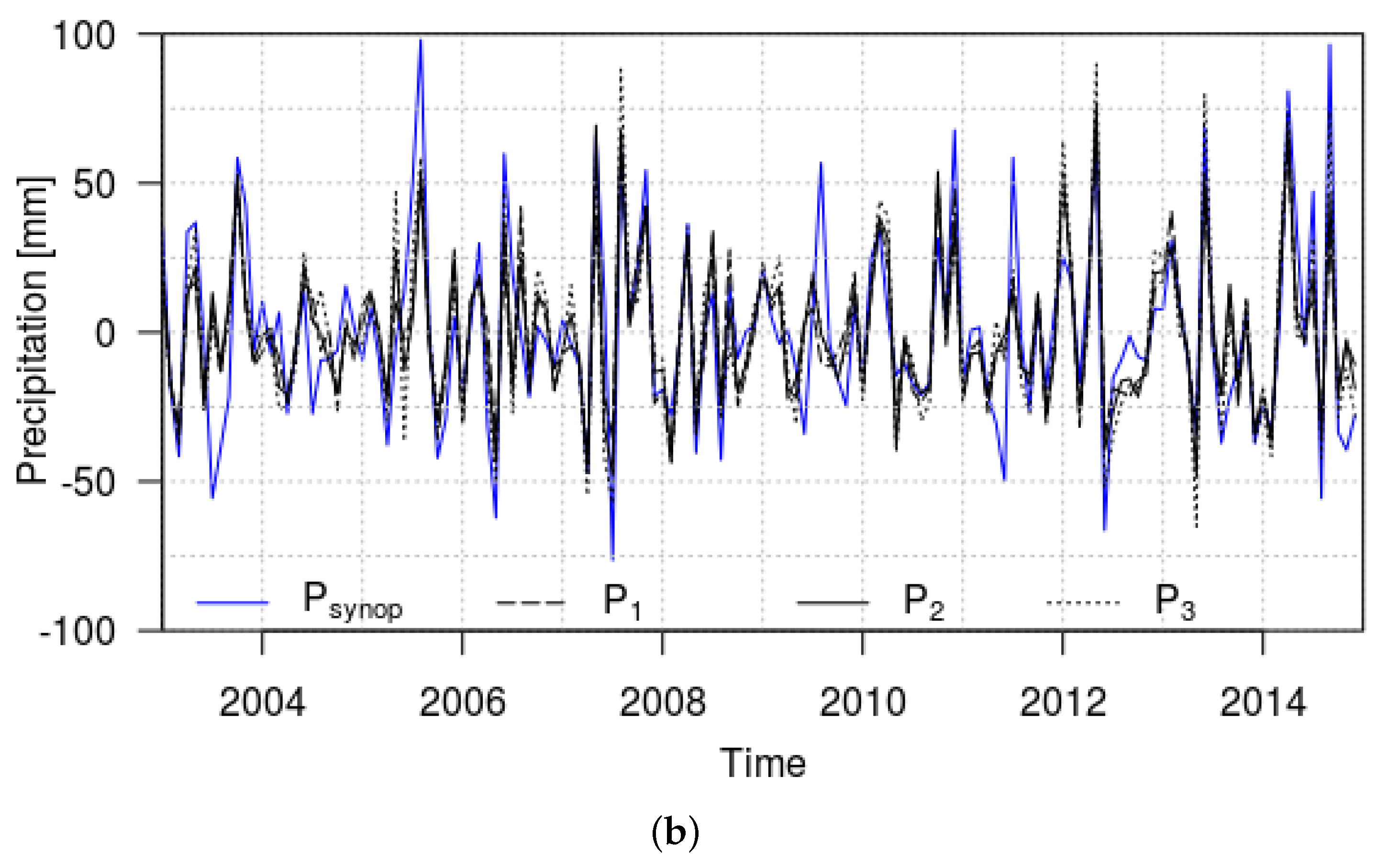
3.3. Comparison between ERA5 and SYNOP Temperature and Precipitation

Figure 6 shows the differences between ERA5 and SYNOP temperature and precipitation for the 2003–2014 period. The results indicated that the ERA5 temperature data generally underestimated the observed temperature at Sofia station with some notable exceptions, such as January 2014 when the ERA5 temperature largely overestimated the observed temperature (Figure 6a). The mean difference between ERA5 and observed temperature was −0.7 ${}^{\circ }$C, −1.2 ${}^{\circ }$C and −1.4 ${}^{\circ }$C, for the three ERA5 points over the 2003–2014 period. It is to be noted that the ERA5 temperature is calculated for three grid points with higher altitude than the SYNOP station. The altitude difference (ERA5 minus SYNOP) is +187, +254 and +253 m asl for the three grid points. This explains why the ERA5 temperature was lower than the observed temperature. In addition, similar tendencies between observed and reanalysis temperature time series were obtained. The computed cross-correlation coefficients between the observed data and the respective ERA5 records for three points were > 0.99. It is interesting that the ERA5 data grid point nearest to the Sofia station exhibited the largest bias. For the precipitation, the mean differences between the ERA5 and SYNOP data were −4.8 mm, −2.7 mm and 8.7 mm for the three points. For the precipitation the correlations between reanalysis and observed data were weaker than for the temperature but still relatively strong, with correlation coefficients of 0.71, 0.77 and 0.83 for the three grid points. Among the three ERA5 grid points the highest correlation coefficient of 0.83 was observed for the point closest to the Sofia station ($P_3$). The reanalysis precipitation data for this point exhibited the largest shift compared to the other points; however this also best reflects the tendencies of the observed precipitation.

Next, the long-term components were extracted and analyzed for the temperature and precipitation time series. In Figure 7a the long-term components of SYNOP temperature and ERA5 temperature for the three chosen locations are compared. All three ERA5 series underestimated the temperature measured at Sofia station due to the different altitudes of the reanalysis and observed data. The higher the difference between altitudes of ERA5 grid points and observed data, the larger the underestimation of the observed temperature. However, the temporal patterns for all temperature records were similar, indicating that ERA5 data tendencies reflect the trends in the observed SYNOP temperature in Sofia. This is also an indication that the SYNOP data were likely assimilated in ERA5 reanalysis. In Figure 7b, the long-term variations of SYNOP precipitation and ERA5 precipitation for the three chosen locations are compared. For 2014 all precipitation long-term components exhibited a rapid increase. The ERA5 data point closest to the Sofia SYNOP station best matched the increasing trend in the observed precipitation. For 2014 both records attained their largest values over the 2003–2014 period. For the other two locations, long-term ERA5 precipitation variations were also similar to the observed precipitation variations. Thus, the year 2014 stands as the year with the largest increase in the long-term component of both the SYNOP and ERA5 precipitation over the studied period.

In Figure 8a, the subseasonal residuals of SYNOP and ERA5 temperatures for the three grid points are compared. The subseasonal residuals of the temperature during the winter months of 2014 were very large, indicating the warm winter. The 2014 winter subseasonal temperature residual anomaly was one of the four largest (2007, 2010, 2011 and 2014) during the 2003–2014 period. In the following months, the subseasonal residuals decreased to moderate values. Temporal patterns of variability for all temperature records were similar despite differences in the mean, indicating that ERA5 tendencies reflect the trends in the observed temperature data from the Sofia SYNOP station. In Figure 8b, the subseasonal residuals of SYNOP and ERA5 precipitation are compared. April 2014 and September 2014 had very large subseasonal precipitation residuals. For these months two of the six largest values of the subseasonal residuals over the studied 2003–2014 period were observed. It is to be noted that in some of the largest floods of the year were recorded in Bulgaria in April and September 2014. Subseasonal precipitation residuals remained positive for most of the year. A secondary peak was observed in July 2014.

3.4. Cross-Correlations between Climate Oscillation Indices and P, T and TWS

In this section the cross-corelations between the climate indices MOI, NAO, AMO and SCAND and precipitation, temperature and TWSA are analyzed. First, seasonal components were removed by decomposition from the time series, which exhibited a pronounced seasonal cycle in temperature, TWSA and AMO, and then the cross-corelation coefficients were computed. None of the chosen indices correlated with temperature. The results for MOI and NAO are presented in

Table 3. Cross-correlation coefficients between the MOI index and time series of and temperature (T), precipitation (P) and terrestrial water storage anomaly (TWSA) from CSR, GFZ and JPL processing centers. The period is 2003–2014. Only values which were significant at the 5% significance level are presented.

Data	Lags in Month
	−6	−5	−4	−3	−2	−1	0	1	2	3	4	5	6
MOI∼T	NS	NS	NS	NS	NS	NS	NS	−0.19	−0.19	NS	NS	NS	NS
MOI∼P	NS	NS	NS	NS	NS	NS	0.25	NS	NS	0.13	NS	NS	NS
MOI∼CSR${}_{twsa}$	0.26	NS	NS	0.20	0.19	0.26	NS	0.16	NS	NS	0.10	NS	NS
MOI∼GFZ${}_{twsa}$	NS	NS	NS	0.19	NS	0.24	NS	NS	NS	NS	NS	NS	NS
MOI∼JPL${}_{twsa}$	0.23	NS	0.25	0.27	0.24	0.31	0.17	0.19	0.19	0.17	0.19	NS	NS

and

Table 4. Cross-correlation coefficients between the NAO index and time series of temperature (T), precipitation (P) and terrestrial water storage anomaly (TWSA) from CSR, GFZ and JPL processing centers. The period is 2003–2014. Only values which were significant at the 5% significance level are presented.

Data	Lags in Month
	−6	−5	−4	−3	−2	−1	0	1	2	3	4	5	6
NAO∼T	NS	NS	NS	NS	NS	NS	NS	NS	NS	NS	NS	NS	NS
NAO∼P	NS	0.24	NS	NS	NS	NS	−0.21	NS	NS	NS	NS	NS	NS
NAO∼CSR${}_{twsa}$	NS	NS	NS	−0.17	−0.21	−0.27	NS	NS	NS	NS	NS	NS	NS
NAO∼GFZ${}_{twsa}$	NS	NS	−0.20	NS	NS	−0.20	NS	NS	NS	NS	NS	NS	NS
NAO∼JPL${}_{twsa}$	NS	−0.15	−0.18	−0.18	−0.19	−0.25	NS	NS	NS	NS	NS	NS	NS

, respectively. They can be summarized as follows: (1) MOI was weakly and positively correlated with precipitation, while the NAO index was weakly and negatively correlated with precipitation; and (2) MOI and the NAO index were weakly to moderately correlated with the TWSA with a one-month lag. Again, MOI was positively correlated with TWSA while the NAO index was negatively correlated with TWSA. The observed correlations were weak but statistically significant (at the 5% significance level) and will be discussed further. The highest positive cross-correlations were observed between MOI and precipitation, with a correlation coefficient of 0.25. The highest negative correlation was between NAO and precipitation (−0.21). This result suggested that climate variability over the Mediterranean Sea and the North Atlantic Ocean influenced precipitation patterns in Bulgaria, which can be explained by the specific cyclogenesis for these regions. The cross-correlation coefficients between MOI and TWSA for a one-month lag were 0.26, 0.24 and 0.31 for CSR data, GFZ data and JPL data, respectively. The obtained correlation coefficients suggested that an above-average value of the MOI is likely to lead to an above average value of TWSA about one month later. Precipitation is also influenced by MOI and responds without a time lag. The cross-correlations between NAO and TWSA with a one-month lag were weak and negative with correlation coefficients of −0.27, −0.20 and −0.25 for CSR data, GFZ data and JPL data, respectively. Thus, there was a tendency in which an above-average value of the NAO index is more likely to be followed by a below-average value of TWSA a month later.

AMO and SCAND indices were not significantly correlated with the studied parameters (temperature, precipitation, TWSA). This result suggested that AMO and SCAND had no significant impact on the climate variability in Bulgaria. In conclusion, there was no strong statistical dependence between the selected climate oscillation indices and the hydrological cycle components precipitation and TWS. However, there was a weak dependence of precipitation and TWSA on two of the studied climate variability indices, namely NAO and MOI.

4. Discussion

One of the most noticeable consequences of climate change will be the impact on the hydrology cycle, i.e., on the water cycling between ocean, atmosphere and land [45]. The extremes in the hydrology cycle, such as dry and wet spells, are already taking place on a regional scale, and understanding their characteristics has been possible in the last two decades by using time series from satellite missions such as GRACE and GRACE-Follow on. The first demonstration of regional GRACE-derived TWS depletion was the 2003 heat wave in Western Europe [46]. Drought occurrence and severity were quantified by Thomas et al. [47] by calculating the magnitude of the deviation of regional and monthly TWSA from the GRACE climatology. A recent work by Boergens et al. [48] studied the 2018–2019 droughts in Central Europe and reported TWS deficits of 73% and 94% of the mean amplitude of seasonal water storage variations, respectively. The study also reported that the water deficits in 2018 and 2019 were the largest observed in GRACE and GRACE-Follow on time series, and importantly those deficits were not expected to recover within one year. According to the European State of the Climate report, compiled by the Copernicus Climate Change Service, in 2018 and partly in 2019 Southeast Europe experienced higher than average summer precipitation [49,50]. The recent and past wet summers in Southeast Europe motivated this quantification of the cross-correlation and possible time lags between different drivers. For the selected case study of the year 2014 we showed that the TWSA annual cycle had a major deviation from the 12-year averaged annual cycle. This is an important finding, which can be used as a criteria for an early warning of wet extremes in Bulgaria. Furthermore, the cross-correlation between TWSA and precipitation had a clearly detectable time lag. Periods with increasing or decreasing precipitation were followed by 3 to 6 months increasing or decreasing TWSA trends in Bulgaria, respectively. This time lag is consistent with a global study by Humphrey et al. [38], which reported a range between 1 and 5 months depending on the region. Our work is the first step towards the estimation of flood potential in Bulgaria. Reager and Famiglietti [51] proposed a flood index by determining repeated maxima in the TWSA, beyond which additional precipitation will have flood generation potential provided increases in runoff or evaporation are not possible. The establishment of the European Gravity Service for Improved Emergency Management (EGSIEM, [52]) prototype was a major development that will support the operational implementation of regional flood early warning systems across Europe. Thus our study is timely and highly relevant to the EGSIEM uptake in Bulgaria and Southeast Europe.

5. Conclusions

Time series analyses of temperature, precipitation and TWS and their correlations with four climate oscillation indices were performed for the 2003–2014 period in order to assess the 2014 wet extremes in Bulgaria. The year 2014 started with negative precipitation anomalies in January and February, which in combination with positive temperature anomalies indicated a drier and warmer winter followed by five consecutive wetter than usual months from March to July and then an even wetter September with precipitation over 200% of the 12-year monthly mean. Anomalies of TWS, derived from three GRACE time series, for the 12-year period had an annual cycle and were mostly positive in the first half of the year from February to June and negative in the second half from July to December. By contrast, the 2014 TWSA was negative from January to April and positive from May to August 2014. Cross-correlations between the long-term trends for the 2003–2014 showed: (1) weak to moderate negative correlations of temperature long-term component with precipitation and TWSA long term components and (2) moderate positive correlations between precipitation long-term component and TWSA long-term component. For the 12-year period, temperature had a positive linear trend of 0.1 ${}^{\circ }$C/year, the precipitation trend was negative (1 mm/year) and TWSA decreased in the range of 2–4 mm/year. The seasonal precipitation cycle peaked in late spring and early summer (May and June). The TWSA peak was in early spring (March and April) while the temperature peak was in summer, i.e., it was out of phase with the TWSA peak.

The long-term variability components of temperature and precipitation from SYNOP and ERA5 showed very good agreement. The year 2014 stood out as the year with the highest increase in the long-term component of the precipitation over the studied 12-year period. For April and September 2014 large subseasonal precipitation residuals were observed, which coincided with a significant number of registered flood events, with a secondary peak observed for July 2014. The MOI and NAO index were weakly correlated with observed precipitation and weakly to moderately correlated with the TWSA. MOI was positively correlated with the precipitation and TWSA, while NAO was negatively correlated with the same parameters. An above-average MOI was more likely to be followed by an above-average TWSA one month later, while an above-average NAO is more likely to be followed by a below-average TWSA one month later.

As demonstrated in this study, the 2014 wet extremes in Bulgaria were closely related to the largest positive precipitation and TWS anomalies recorded for the 12-year period (2003–2014). The presented case study gives a valuable insight about the deviation of the components of annual hydrology cycles during extremely wet years such as 2014. The observed time lags between precipitation and TWSA may be used as a guidance in operational forecasting of wet extremes in Bulgaria. The GRACE time series are essential to the understanding and interpretation of the hydrology cycle, and analysis of the GRACE-Follow on time series will be performed in the near future.

References

1. Zscheischler, J.; Westra, S.; Hurk, B.J.; Seneviratne, S.I.; Ward, P.J.; Pitman, A.; AghaKouchak, A.; Bresch, D.N.; Leonard, M.; Wahl, T.; et al. Future climate risk from compound events. Nat. Clim. Chang. 2018, 8, 469–477. [Google Scholar] [CrossRef]
2. Intergovernmental Panel on Climate Change. Climate Change 2014–Impacts, Adaptation and Vulnerability: Regional Aspects; Cambridge University Press: Cambridge, UK, 2014. [Google Scholar]
3. Several Flood Highlight Climate Change Challenge for Insurer and EU. Available online: https://www.euractiv.com/section/climate-environment/news/severe-floods-highlight-climate-change-challenge-for-insurers-and-eu/ (accessed on 10 May 2020).
4. Serbia Floods 2014. Available online: http://www.ilo.org/wcmsp5/groups/public/-ed_emp/documents/publication/wcms_397685.pdf (accessed on 10 May 2020).
5. Balkan Flood 2014. Available online: http://www.aon.com/czechrepublic/attachments/2014 (accessed on 10 May 2020).
6. Plavšić, J.; Blagojević, B.; Todorović, A.; Despotović, J. Long-term behaviour of precipitation at three stations in Serbia. Acta Hydrotech. 2016, 29, 23–36. [Google Scholar]
7. Stadtherr, L.; Coumou, D.; Petoukhov, V.; Petri, S.; Rahmstorf, S. Record Balkan floods of 2014 linked to planetary wave resonance. Sci. Adv. 2016, 2, e1501428. [Google Scholar] [CrossRef] [PubMed] [Green Version]
8. National Statistical Institute. Flood Events Statistics for the Period 2010–2017. Available online: http://www.nsi.bg/bg/content/2915/ (accessed on 17 July 2020).
9. Stoycheva, A.; Markova, B.; Diakova, A.; Popova, M.; Kirilova, A.; Stoev, K.; Slavchev, M.; Tsekov, G.; Balabanova, S.; Koshnicharov, G.; et al. The 2014 floods and their condisions. Bul. J. Meteo Hydros 2015, 20, 73–105. [Google Scholar]
10. Baldini, L.M.; McDermott, F.; Foley, A.M.; Baldini, J.U. Spatial variability in the European winter precipitation δ18O-NAO relationship: Implications for reconstructing NAO-mode climate variability in the Holocene. Geophys. Res. Lett. 2008, 35. [Google Scholar] [CrossRef]
11. Gallego, M.; García, J.; Vaquero, J. The NAO signal in daily rainfall series over the Iberian Peninsula. Clim. Res. 2005, 29, 103–109. [Google Scholar] [CrossRef]
12. Yiou, P.; Nogaj, M. Extreme climatic events and weather regimes over the North Atlantic: When and where? Geophys. Res. Lett. 2004, 31. [Google Scholar] [CrossRef]
13. Osborn, T.J. Variability and changes in the North Atlantic Oscillation index. In Hydrological, Socioeconomic and Ecological Impacts of the North Atlantic Oscillation in the Mediterranean Region; Springer: Berlin/Heidelberg, Germany, 2011; pp. 9–22. [Google Scholar]
14. Vicente-Serrano, S.M.; López-Moreno, J.I.; Lorenzo-Lacruz, J.; El Kenawy, A.; Azorin-Molina, C.; Morán-Tejeda, E.; Pasho, E.; Zabalza, J.; Beguería, S.; Angulo-Martínez, M. The NAO impact on droughts in the Mediterranean region. In Hydrological, Socioeconomic and Ecological Impacts of the North Atlantic Oscillation in the Mediterranean Region; Springer: Berlin/Heidelberg, Germany, 2011; pp. 23–40. [Google Scholar]
15. Frappart, F.; Ramillien, G. Monitoring groundwater storage changes using the Gravity Recovery and Climate Experiment (GRACE) satellite mission: A review. Remote Sens. 2018, 10, 829. [Google Scholar] [CrossRef] [Green Version]
16. Eicker, A.; Forootan, E.; Springer, A.; Longuevergne, L.; Kusche, J. Does GRACE see the terrestrial water cycle “intensifying”? J. Geophys. Res. Atmos. 2016, 121, 733–745. [Google Scholar] [CrossRef] [Green Version]
17. Zhang, L.; Dobslaw, H.; Stacke, T.; Güntner, A.; Dill, R.; Thomas, M. Validation of terrestrial water storage variations as simulated by different global numerical models with GRACE satellite observations. Hydrol. Earth Syst. Sci. 2017, 21, 821–837. [Google Scholar] [CrossRef] [Green Version]
18. Mircheva, B.; Tsekov, M.; Meyer, U.; Guerova, G. Anomalies of hydrological cycle components during the 2007 heat wave in Bulgaria. J. Atmos. -Sol.-Terr. Phys. 2017, 165, 1–9. [Google Scholar] [CrossRef]
19. Guerova, G.; Simeonov, T.; Yordanova, N. The Sofia University Atmospheric Data Archive (SUADA). Atmos. Meas. Tech. 2014, 7, 2683–2694. [Google Scholar] [CrossRef] [Green Version]
20. Tapley, B.D.; Bettadpur, S.; Ries, J.C.; Thompson, P.F.; Watkins, M.M. GRACE measurements of mass variability in the Earth system. Science 2004, 305, 503–505. [Google Scholar] [CrossRef] [Green Version]
21. Gravity Recovery and Experiment. Available online: http://nasa.gov/Grace (accessed on 10 May 2020).
22. GRACE Follow-On Mission. Available online: http://gracefo.jpl.nasa.gov (accessed on 10 May 2020).
23. Flechtner, F.; Morton, P.; Watkins, M.; Webb, F. Status of the GRACE follow-on mission. In Gravity, Geoid and Height Systems; Springer: Berlin/Heidelberg, Germany, 2014; pp. 117–121. [Google Scholar]
24. Jäggi, A.; Meyer, U.; Lasser, M.; Jenny, B.; Lopez, T.; Flechtner, F.; Dahle, C.; Förste, C.; Mayer-Gürr, T.; Kvas, A.; et al. International Combination Service for Time-Variable Gravity Fields (COST-G); Springer: Berlin/Heidelberg, Germany, 2020. [Google Scholar]
25. Ogimet Weather Information Service. Available online: http://www.ogimet.com (accessed on 10 May 2020).
26. Copernicus Climate Change Service (C3S). Available online: https://climate.copernicus.eu/ (accessed on 10 May 2020).
27. Hurrell, J.W. Decadal trends in the North Atlantic Oscillation: Regional temperatures and precipitation. Science 1995, 269, 676–679. [Google Scholar] [CrossRef] [PubMed] [Green Version]
28. Donat, M.G.; Leckebusch, G.C.; Pinto, J.G.; Ulbrich, U. Examination of wind storms over Central Europe with respect to circulation weather types and NAO phases. Int. J. Climatol. 2010, 30, 1289–1300. [Google Scholar] [CrossRef] [Green Version]
29. North Atlantic Oscillation. Available online: https://crudata.uea.ac.uk/cru/data/nao/ (accessed on 17 July 2020).
30. Conte, M.; Giuffrida, A.; Tedesco, S. The Mediterranean oscillation: Impact on precipitation and hydrology in Italy. In Proceedings of the Conference on Climate and Water, Helsinki, Finland, 11–15 September 1989. [Google Scholar]
31. Palutikof, J.; Conte, M.; Casimiro Mendes, J.; Goodess, C.; Espirito Santo, F. Climate and climatic change. In Mediterranean Desertification and Land Use; Brandt, C.J., Thomes, J.B., Eds.; John Wiley: New York, NY, USA, 1996; pp. 43–86. [Google Scholar]
32. Mediterranean Oscillation Index. Available online: https://crudata.uea.ac.uk/cru/data/moi/ (accessed on 17 July 2020).
33. Atlantic Multidecadal Oscillation. Available online: https://www.esrl.noaa.gov/psd/gcos_wgsp/Timeseries/AMO/ (accessed on 17 July 2020).
34. Knight, J.R.; Folland, C.K.; Scaife, A.A. Climate impacts of the Atlantic multidecadal oscillation. Geophys. Res. Lett. 2006, 33. [Google Scholar] [CrossRef] [Green Version]
35. Barnston, A.G.; Livezey, R.E. Classification, seasonality and persistence of low-frequency atmospheric circulation patterns. Mon. Weather. Rev. 1987, 115, 1083–1126. [Google Scholar] [CrossRef]
36. Climate Prediction Center-Scandinavia. Available online: http://www.cpc.ncep.noaa.gov/data/teledoc/scand.shtml (accessed on 17 July 2020).
37. Cleveland, R.B.; Cleveland, W.S.; Terpenning, I. STL: A seasonal-trend decomposition procedure based on loess. J. Off. Stat. 1990, 6, 3. [Google Scholar]
38. Humphrey, V.; Gudmundsson, L.; Seneviratne, S.I. Assessing global water storage variability from GRACE: Trends, seasonal cycle, subseasonal anomalies and extremes. Surv. Geophys. 2016, 37, 357–395. [Google Scholar] [CrossRef] [Green Version]
39. Sen, P.K. Estimates of the regression coefficient based on Kendall’s tau. J. Am. Stat. Assoc. 1968, 63, 1379–1389. [Google Scholar] [CrossRef]
40. Wilcoxon, F.; Katti, S.; Wilcox, R.A. Critical values and probability levels for the Wilcoxon rank sum test and the Wilcoxon signed rank test. Sel. Tables Math. Stat. 1970, 1, 171–259. [Google Scholar]
41. Hollander, M.; Wolfe, D.A.; Chicken, E. Nonparametric Statistical Methods; John Wiley & Sons: New York, NY, USA, 1973. [Google Scholar]
42. Frappart, F.; Ramillien, G.; Ronchail, J. Changes in terrestrial water storage versus rainfall and discharges in the Amazon basin. Int. J. Climatol. 2013, 33, 3029–3046. [Google Scholar] [CrossRef] [Green Version]
43. de Paiva, R.C.D.; Buarque, D.C.; Collischonn, W.; Bonnet, M.P.; Frappart, F.; Calmant, S.; Mendes, C.A.B. Large-scale hydrologic and hydrodynamic modeling of the Amazon River basin. Water Resour. Res. 2013, 49, 1226–1243. [Google Scholar] [CrossRef] [Green Version]
44. Papa, F.; Güntner, A.; Frappart, F.; Prigent, C.; Rossow, W.B. Variations of surface water extent and water storage in large river basins: A comparison of different global data sources. Geophys. Res. Lett. 2008, 35. [Google Scholar] [CrossRef] [Green Version]
45. Rodell, M.; Beaudoing, H.K.; L’Ecuyer, T.; Olson, W.S.; Famiglietti, J.S.; Houser, P.R.; Adler, R.; Bosilovich, M.G.; Clayson, C.A.; Chambers, D.; et al. The observed state of the water cycle in the early twenty-first century. J. Clim. 2015, 28, 8289–8318. [Google Scholar] [CrossRef]
46. Andersen, O.B.; Seneviratne, S.I.; Hinderer, J.; Viterb, P. GRACE-derived terrestrial water storage depletion associated with the 2003 European heat wave. Geophys. Res. Lett. 2005, 32, L18405. [Google Scholar] [CrossRef]
47. Thomas, B.F.; Famiglietti, J.S.; Landerer, F.W.; Wiese, D.N.; Molotch, N.P.; Argus, D.F. GRACE groundwater drought index: Evaluation of California Central Valley groundwater drought. Remote. Sens. Environ. 2017, 198, 384–392. [Google Scholar] [CrossRef]
48. Boergens, E.; Güntner, A.; Dobslaw, H.; Dahle, C. Quantifying the Central European Droughts in 2018 and 2019 with GRACE-Follow-On. Geophys. Res. Lett. 2020, 47, e2020GL087285. [Google Scholar] [CrossRef]
49. European Wet and Dry Conditions. Available online: https://climate.copernicus.eu/european-wet-and-dry-conditions (accessed on 17 July 2020).
50. ESOTC. Available online: https://climate.copernicus.eu/ESOTC/2019/european-wet-and-dry-conditions (accessed on 17 July 2020).
51. Reager, J.; Gardner, A.; Famiglietti, J.; Wiese, D.; Eicker, A.; Lo, M.H. A decade of sea level rise slowed by climate-driven hydrology. Science 2016, 351, 699–703. [Google Scholar] [CrossRef] [Green Version]
52. Jäggi, A.; Weigelt, M.; Flechtner, F.; Güntner, A.; Mayer-Gürr, T.; Martinis, S.; Bruinsma, S.; Flury, J.; Bourgogne, S.; Steffen, H.; et al. European Gravity Service for Improved Emergency Management (EGSIEM)—from concept to implementation. Geophys. J. Int. 2019, 218, 1572–1590. [Google Scholar] [CrossRef]
Figure 1. Locations of the surface synoptic station (black point), Gravity Recovery and Climate Experiment data sampling region (red circle), Atlantic Multidecadal Oscillation index (red rectangle), North Atlantic Oscillation index (green dots and rectangle), Mediterranean Oscillation Indices index (blue dots and rectangle) and Scandinavian oscillation index (dark green dots and rectangle) domains.
Hydrology 07 00066 g001
Figure 2. (a) Range of SYNOP monthly temperature anomalies over the period 2003–2014 (black bars) and 2014 temperature anomaly (red line with dots) and (b) range of SYNOP monthly precipitation anomalies over the period 2003–2014 (black bars) and 2014 precipitation anomaly (blue line with dots).
Hydrology 07 00066 g002
Figure 3. Range of TWSA (bars) over the period 2003–2014 and 2014 TWSA (line with dots) for (a) CSR; (b) GFZ and (c) JPL data sets.
Hydrology 07 00066 g003aHydrology 07 00066 g003b
Figure 4. Long-term component of temperature (red line), precipitation (blue line) and TWSA (black line) time series produced by seasonal trend decomposition using Loess over the period of 2003–2014.
Hydrology 07 00066 g004
Figure 5. Time series (black line), linear trend (red line) and seasonal trend (dashed black line) of: (a) temperature; (b) precipitation; (c) CSR data for the period 2003–2014; (d) GFZ TWSA data for the period 2003–2014 and (e) JPL TWSA data for the period 2003–2014.
Hydrology 07 00066 g005
Figure 6. ERA5 minus SYNOP difference for: (a) temperature and (b) precipitation. ERA5 point T 1 P 1 is shown with a black line, T 2 P 2 is shown with red circles T 3 P 3 is shown with blue squares.
Hydrology 07 00066 g006aHydrology 07 00066 g006b
Figure 7. Comparison of long-term trends of: (a) temperature from ERA5 (black line, solid, dash and dot) and SYNOP (red line) and (b) precipitation from ERA5 (black line, solid, dash and dot) and SYNOP (blue line) for the 2003–2014 period.
Hydrology 07 00066 g007
Figure 8. Comparison of subseasonal residuals of (a) temperature from ERA5 (black line, solid, dash and dot) and SYNOP (red line) and (b) precipitation from ERA5 (black line, solid, dash and dot) and SYNOP (blue line).
Hydrology 07 00066 g008aHydrology 07 00066 g008b