Article

Assessing the Robustness of Pan Evaporation Models for Estimating Reference Crop Evapotranspiration during Recalibration at Local Conditions

by
Konstantinos Babakos
1,
Dimitris Papamichail
1,
Panagiotis Tziachris
2,
Vassilios Pisinaras
2,
Kleoniki Demertzi
3 and
Vassilis Aschonitis
2,*
1
Department of Hydraulics, Soil Science and Agricultural Engineering, Faculty of Agriculture, Forestry and Natural Environment, Aristotle University of Thessaloniki, 54124 Thessaloniki, Greece
2
Soil and Water Resources Institute, Hellenic Agricultural Organization-Demeter, 57001 Thermi-Thessaloniki, Greece
3
Goulandris Natural History Museum, Greek Biotope/Wetland Centre, 57001 Thermi-Thessaloniki, Greece
*
Author to whom correspondence should be addressed.
Hydrology 2020, 7(3), 62; https://doi.org/10.3390/hydrology7030062
Submission received: 29 July 2020 / Revised: 24 August 2020 / Accepted: 26 August 2020 / Published: 1 September 2020
(This article belongs to the Special Issue Technological Advances in Hydroclimatic Observations)

Abstract

:
A classic method for assessing the reference crop evapotranspiration (ETo) is the pan evaporation (Epan) method that uses Epan measurements and pan coefficient (kp) models, which can be functions of relative humidity (RH), wind speed (u2), and temperature (T). The aim of this study is to present a methodology for evaluating the robustness of regression coefficients associated to climate parameters (RH, u2, and T) in pan method models during recalibration at local conditions. Two years of daily data from April to October (warm season) of meteorological parameters, Epan measurements from class A pan evaporimeter and ETo estimated by ASCE-standardized method for the climatic conditions of Thessaloniki (Greece, semi-arid environment), were used. The regression coefficients of six general nonlinear (NLR) regression Epan models were analyzed through recalibration using a technique called “random cross-validation nonlinear regression RCV-NLR” that produced 1000 random splits of the initial dataset into calibration and validation sets using a constant proportion (70% and 30%, respectively). The variance of the regression coefficients was analyzed based on the 95% interval of the highest posterior density distribution. NLR models that included coefficients with a 95% HPD interval that fluctuates in both positive and negative values were considered nonrobust. The machine-learning technique of random forests (RF) was also used to build a RF model that includes Epan, u2, RH, and T parameters. This model was used as a benchmark for evaluating the predictive accuracy of NLR models but, also, for assessing the relative importance of the predictor climate variables if they were all included in one NLR model. The findings of this study indicated that locally calibrated NLR functions that use only the Epan parameter presented better results, while the inclusion of additional climate parameters was redundant and led to underfitting.

Graphical Abstract

1. Introduction

The parameter of reference crop evapotranspiration ETo describes the maximum water losses that can be achieved by evaporation and transpiration from a field covered by a reference crop (e.g., grass) under no water restrictions, and it is used for water balance analysis and irrigation planning [1,2]. Various methods have been proposed for ETo assessment [1,2,3,4,5,6,7,8,9,10,11], with the most popular being the FAO-56 Penman-Monteith [1] from Food and Agriculture Organization (FAO) of the United Nations, and its updated version, the ASCE-standardized method [2], which reflects the current state-of-the-art, providing ETo estimations for two reference crops (a short and a tall reference crop, which correspond to clipped grass and alfalfa, respectively). The ASCE-standardized method has been proposed by the Task Committee of Environmental and Water Resources Institute (EWRI) of the American Society of Civil Engineers (ASCE) as the most precise method and requires a complete set of the four climatic parameters of temperature, solar radiation, relative humidity, and wind speed, which, in many cases, are not all available.
The problem of data availability can be confronted by other methods of reduced parameters [3,4,5,6,7,8,9,10,11], among which, there is the pan evaporation method that differs from the others, because it requires direct evaporation measurements (Epan) from an evaporimeter. In this method, ETo is commonly calculated as the multiplication product of Epan and a pan coefficient (kp), which depends on the local conditions of the surrounding environment [1]. There are various types of evaporimeters, but the most commonly used type is the class A pan. The class A evaporation pan is circular, 120.7 cm in diameter and 25 cm deep. It is made of galvanized iron (22 gauge) or Monel metal (0.8 mm). The pan is mounted on a wooden open frame platform, which is 15 cm above ground level. The pan must be level. It is filled with water to 5 cm below the rim, and the water level should not be allowed to drop to more than 7.5 cm below the rim. The water should be regularly renewed, at least weekly, to eliminate extreme turbidity. The pan, if galvanized, should be painted annually with aluminum paint [1].
With respect to class A pan evaporation, various regression kp models have been developed, which are functions of various parameters such as relative humidity, wind speed, temperature, and the fetch distance between the pan evaporation and boundary of grass covered or fallow soil surface [12,13,14,15,16,17,18,19,20,21]. The specific regression kp models have been tested in many environments [19,20,21,22,23,24,25,26,27,28,29,30,31,32,33,34,35,36,37,38,39,40,41,42,43,44,45,46,47,48,49,50,51,52,53,54,55,56,57,58,59,60], while, in many cases, their regression coefficients have been recalibrated or their form has been changed (e.g., using machine-learning models) to describe better the local conditions [19,26,33,38,40,41,47,49].
There are four main issues during kp models’ recalibration or formation that should be considered. The first issue is that the predefined forms of kp models are subjected to nonlinear regression analysis (nonlinear regression also includes machine-learning techniques) without investigating if the climate parameters inside a kp model (e.g., RH, u2, and T) have a robust effect.
The second issue is that the regression analysis is usually performed considering the kp as dependent parameter. This approach does not allow a comparative analysis between the effects of Epan and the other climate parameters (e.g., u2, RH, and T), because Epan measurements are embodied in the “measured” kp values. This approach also creates other problems that are associated to the regression analysis. During a regression analysis, an optimization algorithm aims at minimizing the errors between observed and predicted values of the dependent variable, and because of this procedure, the observed kp with larger values have a greater effect on the error measures [61] and, consequently, a greater effect on regulating the regression coefficients. For example, if the measured kp values of colder days (lower ETo) are larger from the respective values of warmer days (higher ETo), which is not unusual [29,36,49], then the final calibrated kp model will perform better at colder days with lower ETo values. It is also worth mentioning that there are uncertainties in the validity of ETo during the cold periods [7] and thus, the kp values of those periods may not be accurate.
The third issue is that the estimated ETo by a complete formula (e.g., ASCE-standardized method) and the measured Epan evaporation are both affected by the same climate parameters, and someone would expect that solely Epan could explain the largest portion of variance in estimated ETo values, especially when there are no observed extreme deviations of meteorological parameters from normal conditions. That means that a model that considers only Epan without the inclusion of other parameters could provide an adequate prediction accuracy (examples of such models are given in [25,35,43,46,47,60], with R2 ranging between ~0.7–0.95), while the other climate parameters may be redundant. The reasons that could explain a low accuracy regression model between ETo and Epan are (a) the selection of a nonappropriate form of the regression model and (b) the introduction of experimental bias during ETo and Epan measurements and, especially, during the measurement of real ETo in lysimeter conditions where additional effects from the soil and the grass crop may occur [62]. It is also worth mentioning that there are very few cases of calibrated kp models using measured ETo from lysimeters [13,15,16,22,24,33], while, in most cases, ETo is calculated using a benchmark method (e.g., ASCE-standardized method) that already uses a full set of climate parameters. Calibrating kp models that include the same climate parameters used for calculating ETo values may also be questionable from a statistical/mathematical point of view.
The fourth issue is that the relationship between ETo and Epan is usually defined a priori by ETo = kp·Epan without investigating if these two parameters are related in a different way.
Considering the above issues, the objective of this study is to propose an integrated methodology for evaluating the robustness of regression coefficients and, consequently, their associated climate parameters that participate in general forms of pan evaporation models during recalibration at local conditions. In this study, the general forms of existing pan evaporation models are used as examples, and they are recalibrated at local conditions based on estimated daily ETo values by the ASCE-standardized method for short grass (equivalent to the FAO-56 method). The proposed methodology that is going to be presented in this study allows to select the important climate parameters (e.g., RH, u2, and T) in combination with Epan measurements for building a robust model for the estimation of ETo at local conditions.

2. Materials and Methods

2.1. Data

Daily meteorological data of temperature (T), relative humidity (RH), solar radiation (Rs), wind speed at 2 m above ground (u2), and precipitation (P) covering the warm-dry cultivation periods (May to September) of the years 2008 and 2009 were obtained by the meteorological station of the Aristotle University Farm (40°32′08″ Ν, 22°59′18″ Ε, ~1 m a.s.l.) in Thessaloniki, Greece (Table 1). The daily values of climate parameters were calculated as mean values of hourly observations of a 24-h period.
The climate data were used for estimating daily ETo based on the ASCE-standardized method [2]. Additionally, daily Epan measurements were obtained during the same period using a class A pan evaporimeter of Monel metal with fetch distance F = 1 m for green upwind fetch (Case A) (Table 1). The data describe adequately the meteorological conditions of the warm-dry season in the Thessaloniki Plain in Greece, where the climate is considered a semi-arid Mediterranean environment. The period of May–September is the period for cultivating summer crops and the period of interest for calculating ETo for irrigation purposes. The records of rainfall days (p > 0) during May–September were also excluded from the analysis, leading to a final number of 212 daily records of meteorological and Epan data.

2.2. Reference Crop Evapotranspiration

ETo was estimated in this study using the ASCE-standardized method at a daily step for short reference crops (clipped grass of 12 cm) by the following function [2]:
ETo = [0.408·Δ(Rn − G) + Cn·γ·u2 (es − ea)/(T + 273.16)]/[Δ + γ(1 + Cd·u2)]
where ΕΤο is the reference crop evapotranspiration (mm d−1), Rn is the net radiation at the crop surface (MJ m−2 d−1), u2 is the mean daily wind speed at 2-m height (m s−1), T is the mean daily air temperature (°C), G is the soil heat flux density at the soil surface (MJ m−2 d−1), es is the mean daily vapor pressure (kPa), ea is the mean daily actual vapor pressure (kPa), Δ is the slope of the saturation vapor pressure-temperature curve (kPa °C−1), γ is the psychrometric constant (kPa °C−1), Cn and Cd are constants, which vary according to the time step, the reference crop type (bulk surface resistance and aerodynamic roughness of the surface), and daytime/nighttime ratio. For short reference crop calculations at daily steps using Equation (1), the following values 900, 0.34, and 0 are considered for Cn, Cd, and G, respectively, as suggested by Allen et al. [1,2], providing equivalent ETo results to the FAO-56 Penman-Monteith equation.

2.3. Pan Evaporation Method and General Forms for Local Conditions

The general equation of the pan evaporation method for estimating reference crop evapotranspiration ETo is the following [63]:
ΕΤo = kp·Epan
where Epan is the measured evaporation from the evaporimeter (mm day−1), and kp is the pan evaporation coefficient. The range of kp values is approximately between 0.35 to 1.1 for various pan types and various local conditions of climates and surrounding environments [14,63].
For the purposes of this study, the kp models of Cuenca [13], Allen and Pruitt [14], Snyder [15], Pereira et al. [16], and Orang [17] were used. These models have been developed for estimating short reference crops based on measurements from class A pan evaporimeters and are given, respectively, by the following equations:
kp = 0.475 − 2.4 × 10⁻⁴u2 + 5.16 × 10⁻³RH + 1.18 × 10⁻³F − 1.6 × 10⁻⁵RH2 − 1.01 × 10⁻⁶F2 − 8 × 10⁻⁹RH2u2 − 1 × 10⁻⁸RH2F
kp = 0.108 − 3.31 × 10⁻⁴u2 + 4.22 × 10⁻²ln(F) + 14.34 × 10⁻²ln(RH) − 6.31 × 10⁻⁴[ln(F)]2ln(RH)
kp = 0.482 − 3.76 × 10⁻⁴u2 + 2.4 × 10⁻²ln(F) + 4.5 × 10⁻³RH
kp = 0.85(Δ + γ)/[Δ + γ(1 + 0.33u2)]
kp = 0.51206 − 3.21 × 10⁻⁴u2 + 31.886 × 10⁻³ln(F) + 28.89 × 10⁻⁴RH
where RH is the mean daily relative humidity (%), u2 is the mean daily wind speed at the height of 2 m above the ground (in km d−1 for Equations (3)–(5) and (7) and in m sec−1 for Equation (6)), and F is the upwind distance from the pan to the border of grass-covered land (m). A difference exists in Equation (6) in comparison to the other kp models, because it is a function of u2 and temperature T (T is included in the Δ parameter), and it is also a ratio without an intercept, where all coefficients are related to u2 and T. An additional important kp model is the one of Raghuwanshi and Wallender [18], but it is not used in this study, because it consists of categorical factors where their classes could not be adequately covered by the dataset of this study for allowing a proper recalibration of all its compartments.
On the other hand, Snyder et al. [25] proposed a sine wave equation for estimating ETo using only Epan adjusted for F = 100 m, which was further modified by Ghare et al. [60], who added an intercept as follows:
ΕΤo = 8.889sin[(Epan/19.2)·(π/2)] + 0.6373
Equation (8) is a quite flexible formula and provides an alternative relation between ETo and Epan compared to the commonly used Equation (2).
The five kp models (Equations (3)–(7)) were transformed to their initial general form in order to analyze the robustness of their regression coefficients and, consequently, the effects of their associated climate parameters (e.g., RH, u2, and T) through regression analysis. In Equations (3)–(7), the fetch distance was F = 1 m, which led to the following simplified general forms, respectively:
kp = a + b·u2 + c·RH + d·RH2 + e·RH2u2 (from Equation (3))
kp = a + b·u2 + c·ln(RH) (from Equation (4))
kp = a + b·u2 + c·RH (from Equations (5) and (7))
kp = a(Δ + γ)/[Δ + γ(b + c·u2)] (from Equation (6))
where a, b, c, d, and e are regression coefficients.
Similarly, the general form of Equation (8), with an intercept according to Ghare et al. [61] for estimating ETo using only Epan, was defined as:
ΕΤo = a·sin[(Epan/b)·(π/2)] + c
Finally, the simple regression tool of STATGRAPHICS Centurion XV software (StatPoint Technologies Inc.) was used in order to assess the optimum linear formula with transformed variables between ETo and Epan. The specific tool analyzes automatically 27 linear formulas with various transformations of the variables (Table S1 in Supplementary Materials), providing the option to the user to choose the best one based on performance metrics. For the dataset of this study, the best transformation for both variables (ETo and Epan) was found to be the following:
ln(ΕΤo) = a + b·ln(Epan) → ΕΤo = exp[a + b·ln(Epan)]
In this study, the second nonlinear form of Equation (14) was used in the comparative analysis of the models.

2.4. Methods of Analysis

2.4.1. Nonlinear Regression with Random Cross-Validation

The robustness of the regression coefficients of the six models (Equations (9)–(14)) was investigated using a random cross-validation nonlinear regression (RCV-NLR) analysis considering ETo as the dependent variable (i.e., the four general nonlinear forms of kp, Equations (9)–(12), were included in Equation (2) for estimating ETo). The RCV-NLR analysis is based on a random splitting of the initial dataset into a calibration set (70% of the records) and a validation set (30% of the records). This random splitting was performed 1000 times, leading to a respective number of calibration and validation pairs of datasets. The RCV-NLR analysis was performed for each one of the six models based on the calibration sets, providing 1000 estimations of their respective regression coefficients. The estimated coefficients of each calibration set were used to validate each model based on the respective validation set. The RCV-NLR was built in R software using the “nls.lm” function of the {minpack.lm} package [64], which includes the Levenberg-Marquardt nonlinear least-squares algorithm.
The range of 1000 solutions of each regression coefficient of calibration and validation procedures was defined by the 95% confidence interval of the highest posterior density (HPD) distribution. The 2.5% and 97.5% thresholds (HPD thresholds), which contain the central 95% interval of the HPD distribution, were estimated in R software using the “p.interval” function of the {LaplacesDemon } package [65], which returns unimodal or multimodal HPD intervals, depending on the form of the probability distributions. Based on the RCV-NLR results, a model was considered robust according to the following rule: “a model is robust only when the 95% HPD intervals of all its regression coefficients preserve a constant sign (+ or -)” (i.e., a 95% HPD that contains positive and negative values of a regression coefficient indicates a nonrobust coefficient and, consequently, a nonrobust model).

2.4.2. Multiple Random Forests

Random forests (RF) [66] is a machine-learning method that is an extension and improvement of the Classification and Regression Trees (CART) method, also called decision trees. RF uses a modification of the bootstrap aggregating technique (bagging), by which a large collection of decorrelated, noisy, approximately unbiased trees are built and averaged in order to reduce the model variance and instability problems [67]. RF is an ensemble method where the aggregation of multiple trees improves the overall prediction accuracy, with both low bias and low variance results [66,68]. Some of the advantages of RF are the ability of modeling high-dimensional nonlinear relationships, resistance to overfitting, relative robustness, estimation of variable importance, and few user-defined parameters [66,67,68,69].
The hyperparameters of a RF model play a significant role in a model’s performance, so the determination of their values is crucial. The hyperparameters that were considered were the number of the regression trees (num.trees), the number of candidate predictors that were randomly sampled (mtry), the proportion of train set that was used for building the model (sample.fraction), and the minimum number of points in the terminal nodes of the regression trees (min.node.size). A number of combinations of various values of hyperparameters was constructed, and by execution of the “ranger” package [70], their optimal set of values was determined (mtry = 3, num.trees = 1000, sample.fraction = 0.7, and min.node.size = 3). The validation set was 30% of the initial dataset, as in the case of RCV-NLR. RF also estimates the predictor variables’ importance. The importance of a predictor variable is calculated as the mean—across all trees—decrease (%) of accuracy, expressed by the % change in Mean Squared Error - MSE (%), on the Out-of-Bag (OOB) sample when the variable is not taken into account by permuting its values randomly and maintaining the others as they were. Using constant optimal values of hyperparameters, the internal random procedures in RF lead every time to different solutions. For this reason, 1000 RF iterations (multiple random forests—MRF) were made in order to make comparisons with the NLR models. The MRF analysis was performed using all the predictor variables (Epan, u2, RH, and T) that participate in Equations (9)–(14). RF is not restricted by the limitations of a predefined nonlinear form and can be used as a benchmark model for evaluating the predictive accuracy of NLR models (e.g., Equations (9)–(14)) but, also, for assessing the relative importance of the predictor climate variables if they were all included in one NLR model.

2.4.3. Models’ Metrics

The metrics of R2 and the root mean square error (RMSE) were estimated for each calibration and validation dataset of the RCV-NLR analysis (Equations (9)–(14)) and OOB and validation dataset of the MRF analysis, leading to 1000 respective estimations of their values for each model. Moreover, 1000 estimations of the slope and intercept of the trend line in the 1:1 plot of observed (ETo-ASCE) vs. predicted (RCV-NLR or MRF) models only using the validation sets were also made as complementary metrics. The 1000 estimations of the metrics R2, RMSE, slope, and intercept were also analyzed through the computation of HPD intervals.

3. Results

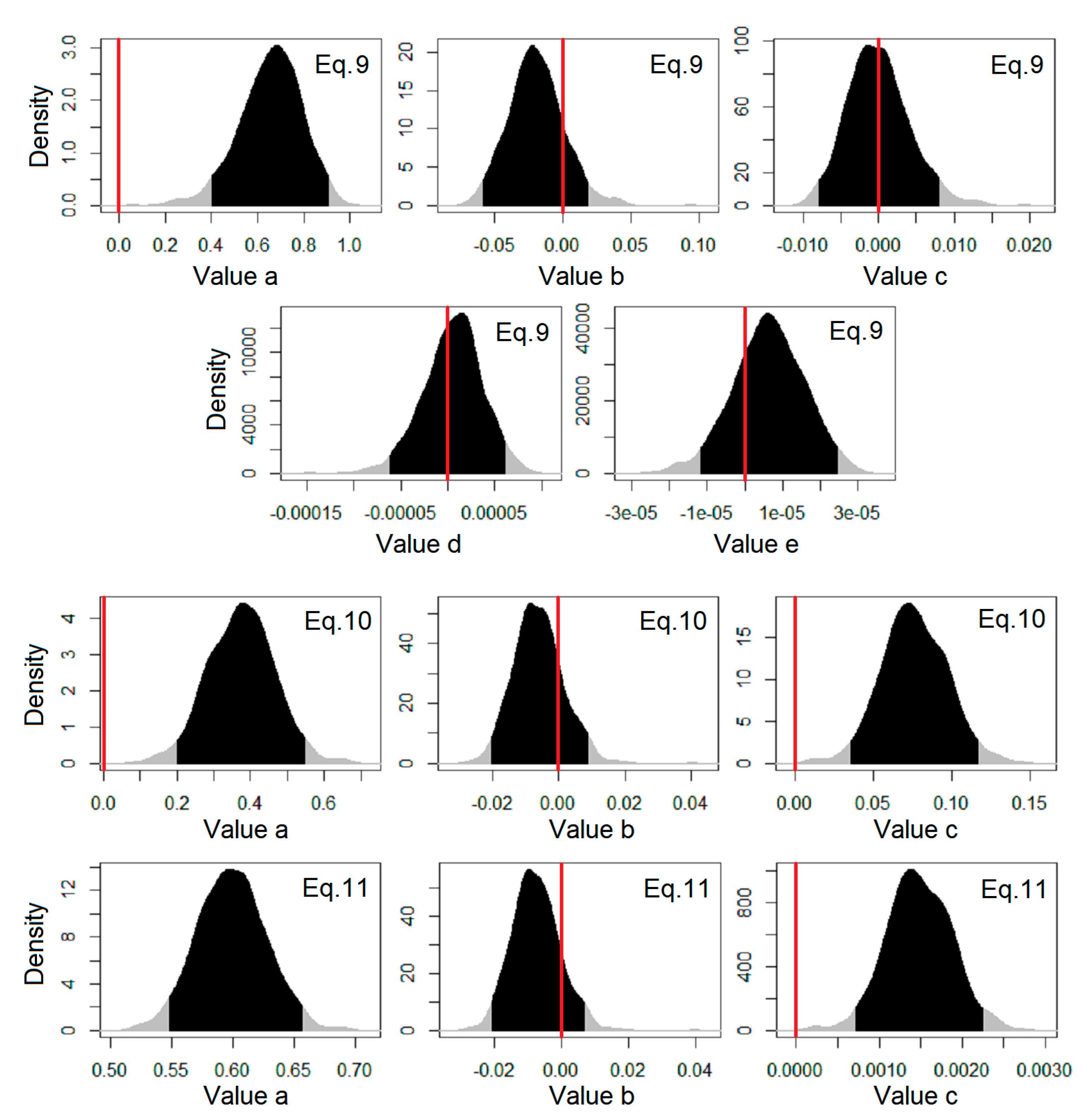
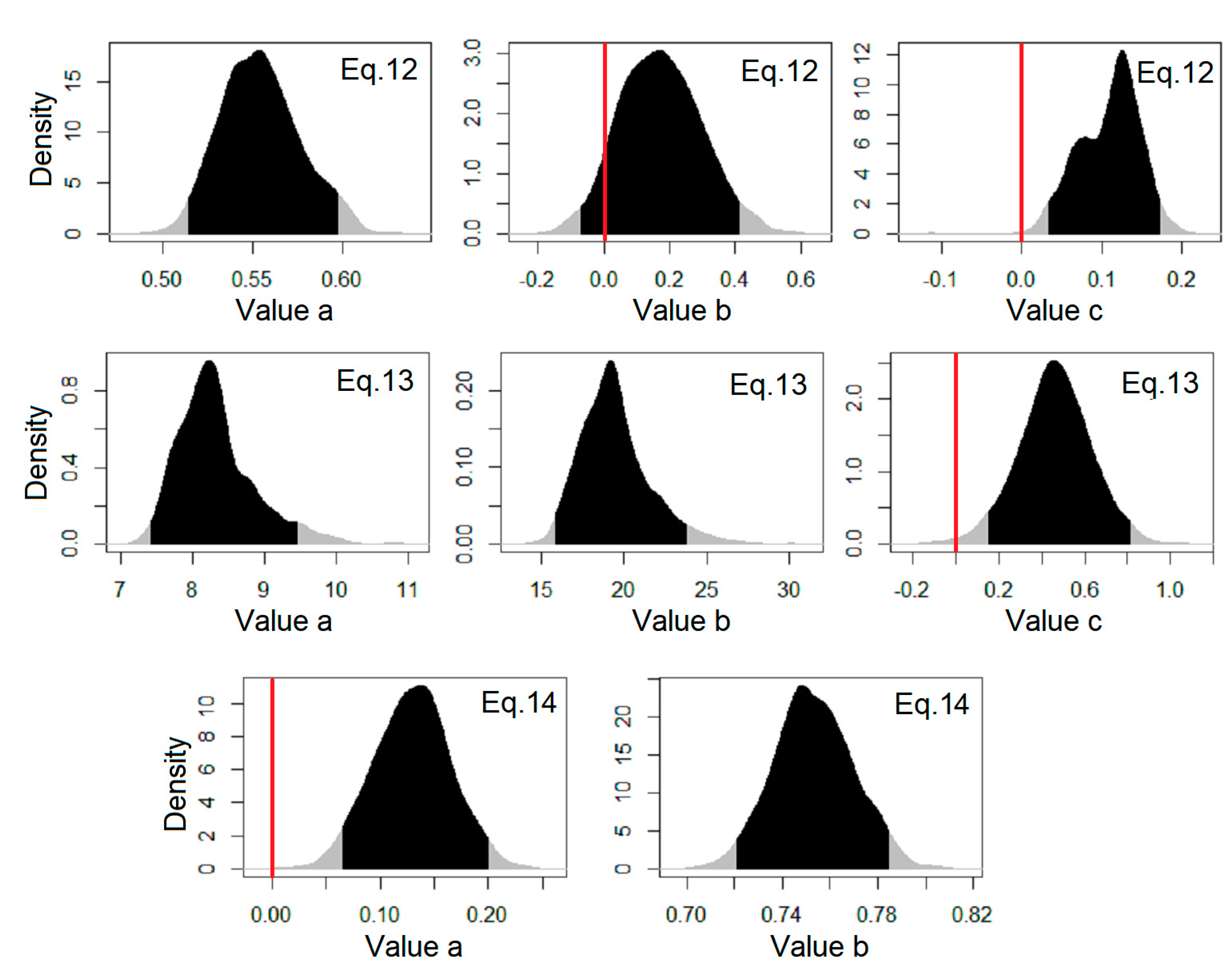
3.1. RCV-NLR Approach

The minimum, mean, maximum, and 2.5% and 97.5% HPD thresholds of the regression coefficients of Equations (9)–(14) derived by the RCV-NLR analysis during calibration are provided in Table S2 (Supplementary Materials). The HPD distributions of the regression coefficients based on their 1000 values are given in Figure 1.
Considering Table S2 and Figure 1, the following were observed:
  • For Equation (9), four out of five regression coefficients (b, c, d, and e coefficients) could not preserve a stable sign inside their 95% HPD interval. These coefficients are associated to RH and u2 based on the specific kp model.
  • For both Equations (10) and (11), one out of three regression coefficients (b coefficient for both cases) could not preserve a stable sign inside its 95% HPD interval. This coefficient is associated to u2 in both kp models.
  • For Equation (12), one out of three regression coefficients (b coefficient) could not preserve a stable sign inside its 95% HPD interval. Due to the complex form of Equation (12), this coefficient is associated to all climate parameters that participate in the specific kp model.
  • For Equations (13) and (14), all their coefficients presented a stable sign inside their 95% HPD intervals.
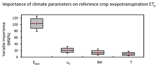
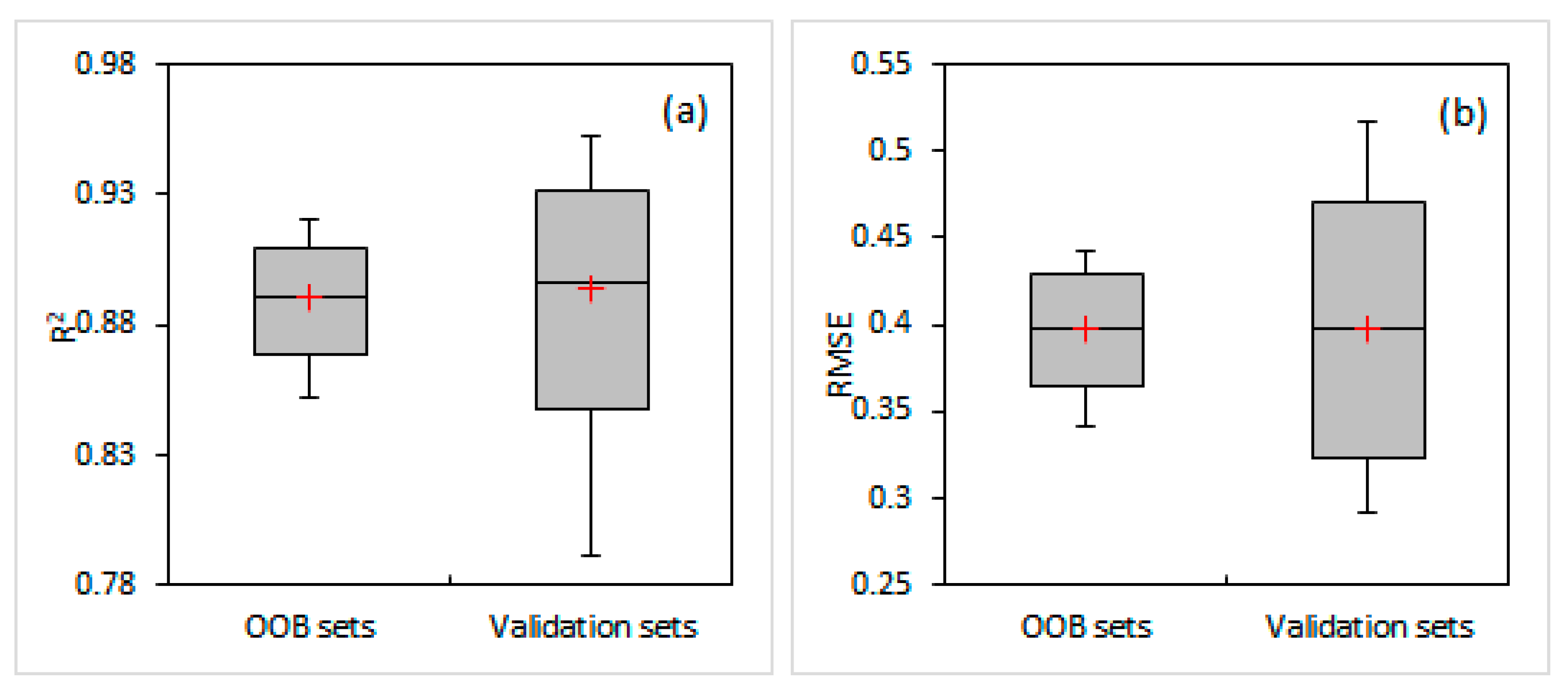
Considering the results of Table S2 and Figure 1, the rule of a constant sign in the 95% HPD interval of all regression coefficients is violated in all models except those that use only the Epan parameter (Equations (13) and (14)). Based on this rule, these two models are expected to be more robust than the other four models (Equations (9)–(12)). This suggestion is verified by the results of R2 and RMSE in the calibration and validation procedures (Table S3 and Figure 2). Figure 2 shows an alternative way to present the HPD distributions using modified box-whisker plots with boxes adjusted to the 95% HPD interval. These plots allow an easier visual comparison of the models’ metrics. The results of Figure 2 show that the models of Equations (13) and (14) present higher R2 and lower RMSE values than the other four models (Equations (9)–(12)) in both calibration (Figure 2a,c) and validation (Figure 2b,d) procedures. The results of Equations (13) and (14) are quite similar, with a slight better performance of Equation (13) (mean R2 = 0.872 and mean RMSE = 0.429 mm d−1 during calibration and mean R2 = 0.866 and mean RMSE = 0.443 mm d−1 during validation), because it has three regression coefficients instead of two, as in the case of Equation (14).

3.2. MRF Approach

The minimum, mean, maximum, and 2.5% and 97.5% HPD thresholds of R2 and RMSE during the OOB and validation procedures of the MRF approach are provided in the modified box-whisker plots of Figure 3a,b, respectively. Their respective values are provided in Table S4 of the Supplementary Materials. The performance of the MRF modeling approach that uses the full set of variables (i.e., Epan, u2, RH, and T) was generally better than the RCV-NLR models, according to the R2 and RMSE metrics (mean R2 = 0.891 and mean RMSE = 0.398 mm d−1 during the OOB procedure and mean R2 = 0.894 and mean RMSE = 0.398 mm d−1 during validation of the MRF).
The respective modified box-whisker plots of the variables’ importance are also provided in Figure 4 and their respective values in Table S5 of the Supplementary Materials. Based on Figure 4 and Table S5, the importance of the variables follows the order Epan > u2 > RH > T, with the MSE% values of Epan being at least five times greater than the rest of the parameters.

3.3. Trend Line (Slope and Intercept) of Observed vs. Predicted ETo Values from 1:1 Plots Based on the Validation Datasets of All Models

The minimum, mean, maximum, and 2.5% and 97.5% HPD thresholds of the slopes and intercepts of the trend lines of the observed vs. predicted ETo values from 1:1 plots were estimated for all the validation cases from the RCV-NLR analysis of Equations (9)–(14) and MRF analysis (Figure 5a,b, Table S6) (in all cases, the validation data are the 30% of the initial dataset). The mean values and the 95% HPD intervals of the slopes and intercepts (Figure 5) showed that the ETo predictions of Equations (13) and (14) are better distributed along the perfect fit line of 45 degrees in comparison to the rest RCV-NLR models and the MRF model.

4. Discussion

4.1. Testing the Inclusion of Meteorological Parameters as Independent Variables in the Epan Methodology

The results of this study showed that the decision to include additional meteorological parameters in the Epan methodology for assessing ETo or to use existing kp models that already use meteorological parameters should be tested with more than one methodology before their use. The advantages and disadvantages of each methodology used in this study can be summarized as follows:
  • The RCV-NLR method with various existing models has the advantage of analyzing the HPD interval of the coefficients, allowing to derive conclusions about the effects of their associated parameters (e.g., RH, u2, and T). On the other hand, this method has the following disadvantages: (a) it is based on predefined nonlinear models that are formed by the user and may not be efficient enough to capture the responses of the dependent variable, and (b) in some cases, the form of the nonlinear models is complex, and the effect of the regression coefficient cannot be easily interpreted (e.g., coefficients of Equation (12)).
  • The MRF method has the following advantages: (a) it is a machine-learning technique that is not restricted by predefined nonlinear forms by the user, (b) its predictions can be used as a measure of the predictive accuracy of typical NLR models, and (c) it provides the relative importance of the parameters. On the other hand, this method has the following disadvantages: (a) an RF model cannot be visualized as a function that is easily applicable by others, and (b) it is impossible to derive information that could explain whether an independent variable positively or negatively affects the dependent variable.
Considering the above, it is crucial to combine the two methodologies in order to derive an integrated conclusion that will allow the selection of the optimum NLR or RF model.

4.2. Effect of the Nonlinear Form on the Importance of Independent Variables

The results of this study showed that different forms of a nonlinear model affect differently the robustness of a regression coefficient and, consequently, the robustness of its associated independent variable. For example, the regression coefficient c in Equations (10) and (11) is associated to the RH and is robust according to the 95% HPD interval rule, while, in Equation (9), all the regression coefficients that are associated to the RH (i.e., the c, d, and e coefficients) are not robust (Figure 1). As regards u2, its respective coefficient b is not robust in Equations (9)–(11) due to the positive and negative values in the respective 95% HPD intervals. Considering the above, someone could agree that RH presents a more clear and robust effect on ETo in the majority of NLR cases than u2, according to the RCV-NLR analysis, but this suggestion is opposite to the results of the MRF analysis, since the importance of the u2 variable is greater than the one of RH (Figure 4). These results highlight the limitations of NLR models to capture correctly the effect of an independent variable.

4.3. Is It Really Needed to Include Climate Parameters in Epan Methodology for Estimating ETo?

The variables’ importance provided by MRF analysis and the small difference in statistical metrics (R2 and RMSE) between the MRF and Equations (13) and (14) showed that simple NLR models that use only Epan can reach a very satisfactory performance when they are calibrated for local conditions. Moreover, it was observed that the inclusion of additional climate parameters in NLR models may lead to underfitting, since Equations (9)–(12) showed poorer performance than Equations (13) and (14). The MRF analysis also showed the dominance of the Epan variable over the other three parameters (u2, RH, and T), even though the dependent variable (ETo of the ASCE-standardized method) was estimated directly by them. This result can be easily justified by the fact that Epan includes/combines all the effects of the rest variables, indicating that their inclusion may be redundant. Our opinion is that the general forms of Equations (13) and (14) or some of the alternative general equations provided in Table S1 can describe satisfactorily the relation between ETo and Epan when they are calibrated for local conditions. The mean values and 95% HPD intervals of the slopes and intercepts that were derived from the 1:1 plots of the observed vs. predicted ETo values of the validation datasets (Figure 5) also showed that the ETo predictions of Equations (13) and (14) are better distributed along the perfect fit line of 45 degrees in comparison to the MRF model and the rest of the RCV-NLR models. This indicates that MRF may be the most powerful model to minimize the overall error (in terms of RMSE and R2), but it is not so robust at larger and smaller ETo values, probably due to bias from the inclusion of the climate parameters of u2, RH, and T.

4.4. Future Studies for Different Fetch and Different Climate Types

The precalibrated models of Equations (3)–(9) were given in this study in order to provide the source of different NLR forms, while the general forms that occurred (Equations (9)–(14)) were free from F, because they had to be recalibrated for a specific environment with constant fetch conditions. On the other hand, in the case where recalibration should be performed using data that include different fetch conditions, then the same analysis should be performed with the inclusion of F in the general forms of Equations (9)–(14). Such an analysis would be interesting, allowing also to assess the robustness of F parameter through analysis on its associated regression coefficients. The result of such an analysis regarding the robustness of the F parameter is unknown, and future studies should also focus on this issue.
The analysis of this study is based only on two years during the period May–September due to the temporary installation of a class A pan in the context of a parallel evapotranspiration experiment with lysimeters cropped, with flooded rice during the same period [71,72]. We believe that the selected dataset fulfills the requirements for supporting the results and conclusions of this study, despite the fact that it covers a small period and despite the fact that it describes the conditions of one climate type (semi-arid environment). Our opinion is based on the high variability of the daily records of the parameters (T, u2, RH, Epan, and ETo) that were used in this study, which are provided in the form of histograms (Figure S1 in the Supplementary Materials). The large coverage and the distribution of these parameters is adequate for supporting robust conclusions about the effects of the T, u2, and RH parameters in pan method models for the specific climate type, but future studies are also required to prove these findings for other climate types.

5. Conclusions

This study presented an integrated methodology for evaluating the robustness of regression coefficients associated to climate parameters (RH, u2, and T) in pan method models during recalibration at local conditions. The results of this study showed that:
(a)
the typical formula of Equation (2), with the use of a predefined form of a kp model with locally calibrated coefficients, may not be the optimum solution for estimating ETo. In the case of using such models, the calibration should be performed using as a dependent variable the ETo and not the “measured” kp (defined as the ratio ETo/Epan).
(b)
the inclusion of climate parameters (e.g., u2, RH, and T) in pan method models (NLR, MRF, etc.) for estimating ETo may lead to underfitting and can be considered questionably from a statistical/mathematical point of view when ETo is not measured but computed by a formula that is based on the same climate parameters.
(c)
locally calibrated nonlinear regression functions for estimating ETo, which use only the Epan parameter, can have high predictive accuracy without the inclusion of additional climate parameters and can provide more balanced predictions along the perfect fit line of 45 degrees in 1:1 plots of observed vs. predicted ETo.
The findings of the specific study should also be investigated for different fetch and different climate types in future studies.

Supplementary Materials

The following are available online at https://www.mdpi.com/2306-5338/7/3/62/s1: Table S1: 27 cases of linear models with transformed variables. The performance of these models is automatically tested by StatGraphics Centurion XV software. Table S2: Minimum, mean, maximum, and 2.5% and 97.5% HPD thresholds of regression coefficients of Equations (9)–(14) derived by the RCV-NLR analysis during calibration (for Equations (9)–(12), the regression was made based on Equation (2) using ETo as the dependent variable). Table S3: Minimum, mean, maximum, and 2.5% and 97.5% HPD thresholds of R2 and RMSE during calibration and validation for the six models Equations (9)–(14) based on RCV-NLR. Table S4: Minimum, mean, maximum, and 2.5% and 97.5% HPD thresholds of R2 and RMSE during OOB and validation procedures for the MRF modeling approach. Table S5: Minimum, mean, maximum, and 2.5% and 97.5% HPD thresholds of the variables’ importance expressed as MSE% for the MRF modeling approach. Table S6: Minimum, mean, maximum, and 2.5% and 97.5% HPD thresholds of slopes and intercepts of the trend lines of observed vs. predicted ETo values from 1:1 plots estimated for all the validation cases from the RCV-NLR analysis of Equations (9)–(14) and the MRF analysis. Figure S1: Frequency histograms of the 212 records of T, u2, RH, Epan, and ETo used in this study.

Author Contributions

Conceptualization, K.B., V.A. and D.P.; methodology, K.B., V.A., P.T. and V.P.; software, K.B., V.A., P.T., V.P. and K.D.; formal analysis, K.B., V.A., P.T., V.P., K.D. and D.P.; resources, V.A.; data curation, V.A., K.B. and K.D.; writing—original draft preparation, K.B., V.A., P.T., V.P., K.D. and D.P.; writing—review and editing, K.B., V.A., P.T., V.P., K.D. and D.P.; and supervision, V.A. and D.P. All authors have read and agreed to the published version of the manuscript.

Funding

This research received no external funding.

Conflicts of Interest

The authors declare no conflict of interest.

References

  1. Allen, R.G.; Pereira, L.S.; Raes, D.; Smith, M. Crop Evapotranspiration: Guidelines for Computing Crop Water Requirements. Irrigation and Drainage Paper 56; Food and Agriculture Organization of the United Nations: Rome, Italy, 1998. [Google Scholar]
  2. Allen, R.G.; Walter, I.A.; Elliott, R.; Howell, T.; Itenfisu, D.; Jensen, M. The ASCE Standardized Reference Evapotranspiration Equation; Final Report (ASCE–EWRI); Task Committee on Standardization of Reference Evapotranspiration, Environmental and Water Resources Institute of the American Society of Civil Engineers: Reston, VA, USA, 2005. [Google Scholar]
  3. Priestley, C.H.B.; Taylor, R.J. On the assessment of surface heat flux and evaporation using large–scale parameters. Mon. Weather Rev. 1972, 100, 81–92. [Google Scholar] [CrossRef]
  4. Hargreaves, G.H.; Samani, Z.A. Estimating potential evapotranspiration. J. Irrig. Drain Eng. 1982, 108, 223–230. [Google Scholar]
  5. Itenfisu, D.; Elliott, R.L.; Allen, R.G.; Walter, I.A. Comparison of reference evapotranspiration calculations as part of the ASCE standardization effort. J. Irrig. Drain Eng. 2003, 129, 440–448. [Google Scholar] [CrossRef]
  6. Alexandris, S.; Kerkides, P.; Liakatas, A. Daily reference evapotranspiration estimates by the “Copais” approach. Agric. Water Manage. 2006, 82, 371–386. [Google Scholar] [CrossRef]
  7. Aschonitis, V.G.; Papamichail, D.; Demertzi, K.; Colombani, N.; Mastrocicco, M.; Ghirardini, A.; Castaldelli, G.; Fano, E.-A. High–resolution global grids of revised Priestley–Taylor and Hargreaves–Samani coefficients for assessing ASCE–standardized reference crop evapotranspiration and solar radiation. Earth Syst. Sci. Data 2017, 9, 615–638. [Google Scholar] [CrossRef] [Green Version]
  8. Wang, K.; Dickinson, R.E. A review of global terrestrial evapotranspiration: Observation, modeling, climatology, and climatic variability. Rev. Geophys. 2012, 50, 1–54. [Google Scholar] [CrossRef]
  9. McMahon, T.A.; Peel, M.C.; Lowe, L.; Srikanthan, R.; McVicar, T.R. Estimating actual, potential, reference crop and pan evaporation using standard meteorological data: A pragmatic synthesis. Hydrol. Earth Syst. Sci. 2013, 17, 1331–1363. [Google Scholar] [CrossRef] [Green Version]
  10. Valipour, M. Analysis of potential evapotranspiration using limited weather data. Appl. Water Sci. 2017, 7, 187–197. [Google Scholar] [CrossRef] [Green Version]
  11. Valiantzas, J.D. Temperature- and humidity-ased simplified Penman’s ET0 formulae. Comparisons with temperature-based Hargreaves-Samani and other methodologies. Agric. Water Manage. 2018, 208, 326–334. [Google Scholar] [CrossRef]
  12. Frevert, D.K.; Hill, R.W.; Braaten, B.C. Estimation of FAO evapotranspiration coefficients. J. Irrig. Drain. Eng. 1983, 109, 265–270. [Google Scholar] [CrossRef]
  13. Cuenca, R.H. Irrigation System Design: An Engineering Approach; Prentice Hall: Englewood Cliffs, NJ, USA, 1989; p. 552. [Google Scholar]
  14. Allen, R.G.; Pruitt, W.O. FAO-24 reference evapotranspiration factors. J. Irrig. Drain. Eng. 1991, 117, 758–773. [Google Scholar] [CrossRef]
  15. Snyder, R.L. Equation for evaporation pan to evapotranspiration conversions. J. Irrig. Drain. Eng. 1992, 118, 977–980. [Google Scholar] [CrossRef]
  16. Pereira, A.R.; Villanova, N.; Pereira, A.S.; Baebieri, V.A. A model for the class—A pan coefficient. Agric. For. Meteorol. 1995, 76, 75–82. [Google Scholar] [CrossRef]
  17. Orang, M. Potential Accuracy of the Popular Non-Linear Regression Equations for Estimating Pan Coefficient Values in the Original and FAO-24 Tables. Unpublished Report; California Department of Water Resources: Sacramento, CA, USA, 1998. [Google Scholar]
  18. Raghuwanshi, N.S.; Wallender, W.W. Converting from pan evaporation to evapotranspiration. J. Irrig. Drain. Eng. 1998, 124, 275–277. [Google Scholar] [CrossRef]
  19. Grismer, M.E.; Orang, M.; Snyder, R.; Matyac, R. Pan evaporation to reference evapotranspiration conversion methods. J. Irrig. Drain. Eng. 2002, 128, 180–184. [Google Scholar] [CrossRef]
  20. Wahed, M.H.A.; Snyder, R.L. Simple equation to estimate reference evapotranspiration from evaporation pans surrounded by fallow soil. J. Irrig. Drain. Eng. 2008, 134, 425–429. [Google Scholar] [CrossRef]
  21. Tabari, H.; Mark, E.; Trajkovic, S. Comparative analysis of 31 reference evapotranspiration methods under humid conditions. Irrig. Sci. 2013, 31, 107–117. [Google Scholar] [CrossRef]
  22. Katul, G.G.; Cuenca, R.H.; Grebet, P.; Wright, J.L.; Pruitt, W.O. Analysis of evaporative flux data for various climates. J. Irrig. Drain. Eng. 1992, 118, 601–618. [Google Scholar] [CrossRef]
  23. Irmak, S.; Haman, D.Z.; Jones, J.W. Evaluation of Class A pan coefficients for estimating reference evapotranspiration in humid location. J. Irrig. Drain. Eng. 2002, 128, 153–159. [Google Scholar] [CrossRef]
  24. Sentelhas, P.C.; Folegatti, M.V. Class A pan coefficients (Kp) to estimate daily reference evapotranspiration (ETo). Rev. Bras. Eng. Agric. Amb. 2003, 7, 111–115. [Google Scholar] [CrossRef] [Green Version]
  25. Snyder, R.L.; Orang, M.; Matyac, S.; Grismer, M.E. Simplified estimation of reference. Evapotranspiration from pan evaporation data in california. J. Irrig. Drain. Eng. 2005, 131, 249–253. [Google Scholar] [CrossRef]
  26. Khoob, A.R.; Behbahani, S.; Nazarifar, M.H. Developing pan evaporation to grass reference evapotranspiration conversion model a case study in Khuzestan Province. J. Appl. Sci. 2007, 7, 936–941. [Google Scholar] [CrossRef]
  27. Gundekar, H.G.; Khodke, U.M.; Sarkar, S.; Rai, R.K. Evaluation of pan coefficient for reference crop evapotranspiration for semi-arid region. Irrig. Sci. 2008, 26, 169–175. [Google Scholar] [CrossRef]
  28. Xing, Z.; Chow, L.; Meng, F.-R.; Rees, H.W.; Monteith, J.; Lionel, S. Testing reference evapotranspiration estimation methods using evaporation pan and modeling in maritime region of Canada. J. Irrig. Drain. Eng. 2008, 134, 417–424. [Google Scholar] [CrossRef]
  29. Ghare, A.D.; Porey, P.D. Estimation of reference evapotranspiration of Nagpur region using simplified approach. In Proceedings of the 1st International Conference on Emerging Trends in Engineering and Technology, ICETET 2008, Nagpur, India, 16–18 July 2008; pp. 1022–1028. [Google Scholar]
  30. Rahimikhoob, A. An evaluation of common pan coefficient equations to estimate reference evapotranspiration in a subtropical climate (north of Iran). Irrig. Sci. 2009, 27, 289–296. [Google Scholar] [CrossRef]
  31. Sabziparvar, A.-A.; Tabari, H.; Aeini, A.; Ghafouri, M. Evaluation of class a pan coefficient models for estimation of reference crop evapotranspiration in cold semi-arid and warm arid climates. Water Resour. Manag. 2010, 24, 909–920. [Google Scholar] [CrossRef]
  32. Esteves, B.S.; Mendonça, J.C.; Sousa, E.F.; Bernardo, S. Evaluation of “Class A” pan coefficients to estimate the referential evapotranspiration in Campos dos Goytacazes, RJ. Rev. Brasil. Engenh. Agric. Amb. 2010, 14, 274–278. [Google Scholar] [CrossRef]
  33. Trajkovic, S.; Kolakovic, S. Comparison of simplified pan-based equations for estimating reference evapotranspiration. J. Irrig. Drain. Eng. 2010, 136, 137–140. [Google Scholar] [CrossRef]
  34. Ditthakit, P.; Chinnarasri, C. Estimation of pan evaporation coefficient using neuro-genetic approach. Am. J. Environ. Sci. 2011, 7, 397–401. [Google Scholar] [CrossRef] [Green Version]
  35. Cunha, A.R. Calculation of the Class—A pan coefficient in greenhouse and field by different methods [Coeficiente do tanque Classe A obtido por diferentes métodos em ambiente protegido e no campo]. Semin. Cienc. Agrar. 2011, 32, 451–464. [Google Scholar] [CrossRef] [Green Version]
  36. Aschonitis, V.G.; Antonopoulos, V.Z.; Papamichail, D. Evaluation of pan coefficient equations in a semi-arid mediterranean environment using the ASCE—Standardized penman-monteith method. Agric. Sci. 2012, 3, 58–65. [Google Scholar] [CrossRef] [Green Version]
  37. Mohammadi, M.; Ghahraman, B.; Davary, K.; Liaghat, A.M.; Bannayan, M. Pan coefficient (Kp) estimation under uncertainty on fetch. Meteorol. Atmos. Phys. 2012, 117, 73–83. [Google Scholar] [CrossRef]
  38. Sabziparvar, A.A.; Shadmani, M. Evaluation of pan coefficients from ANN, ANFIS, and empirical methods, for estimation of daily reference evapotranspiration. J. Earth Space Phys. 2012, 38, 229–240. [Google Scholar]
  39. Kaya, S.; Evren, S.; Dasci, E.; Bakir, H.; Adiguzel, M.C.; Yilmaz, H. Evaluation of pan coefficient for reference crop evapotranspiration for Igdir region of Turkey. J. Food Agric. Environ. 2012, 10, 987–991. [Google Scholar]
  40. Duan, C.; Miao, Q.; Cao, W.; Wang, Y. Estimation of reference crop evapotranspiration by Chinese pan evaporation in Northwest China. Trans. Chin. Soc. Agric. Eng. 2012, 28, 94–99. [Google Scholar] [CrossRef]
  41. Ditthakit, P.; Chinnarasri, C. Estimation of pan coefficient using M5 model tree. Am. J. Environ. Sci. 2012, 8, 95–103. [Google Scholar] [CrossRef] [Green Version]
  42. Sahoo, B.; Walling, I.; Deka, B.C.; Bhatt, B.P. Standardization of reference evapotranspiration models for a subhumid valley rangeland in the Eastern Himalaya. J. Irrig. Drain. Eng. 2012, 138, 880–895. [Google Scholar] [CrossRef]
  43. Pradhan, S.; Sehgal, V.K.; Das, D.K.; Bandyopadhyay, K.K.; Singh, R. Evaluation of pan coefficient methods for estimating FAO-56 reference crop evapotranspiration in a semi-arid environment. J. Agrometeorol. 2013, 15, 1–4. [Google Scholar]
  44. da Cunha, P.C.R.; do Nascimento, J.L.; da Silveira, P.M.; Júnior, J.A. Efficiency of methods for calculating class A pan coefficients to estimate evapotranspiration reference [Eficiência de métodos para o cálculo de coeficientes do tanque classe A na estimativa da evapotranspiração de referência]. Pesqui. Agropecu. Trop. 2013, 43, 114–122. [Google Scholar] [CrossRef]
  45. Rahimikhoob, A.; Asadi, M.; Mashal, M. A comparison between conventional and M5 Model Tree methods for converting pan evaporation to reference evapotranspiration for semi-arid region. Water Resour. Manag. 2013, 27, 4815–4826. [Google Scholar] [CrossRef]
  46. Heydari, M.M.; Heydari, M. Evaluation of pan coefficient equations for estimating reference crop evapotranspiration in the arid region. Arch. Agron. Soil. Sci. 2014, 60, 715–731. [Google Scholar] [CrossRef]
  47. Zhao, L.W.; Zhao, W.Z. Evapotranspiration of an oasis-desert transition zone in the middle stream of Heihe River, Northwest China. J. Arid Land 2014, 6, 529–539. [Google Scholar] [CrossRef]
  48. Pereira, P.C.; Da Silva, T.G.F.; Silva, S.M.S.E.; Da Neto, J.F.C.; De Morais, J.E.F. Evaluation and applicability of the class A pan coefficient in the middle Pajeu, Pernambuco [Avaliação e aplicabilidade do coeficiente do tanque classe “a” no médio pajeú, pernambuco]. Rev. Caatinga 2014, 27, 131–140. [Google Scholar]
  49. Bhartiya, K.M.; Ghare, A.D. Relative humidity based model for estimation of reference evapotranspiration for western plateau and hills region of India. Water Resour. Manag. 2014, 28, 3355–3364. [Google Scholar] [CrossRef]
  50. Peixoto, T.D.C.; Levien, S.L.A.; Bezerra, A.H.F.; Sobrinho, J.E. Evaluation of different methodologies of class a pan ΕΤo calculation in Μossoró, RN, Brazil [Avaliação de diferentes metodologias de estimativa da eto baseadas no tanque classe a, em mossoró, RN-1]. Rev. Caatinga 2014, 27, 58–65. [Google Scholar]
  51. Bayatvarkeshi, M.; Abyaneh, H.Z. Validating pan coefficient equations to estimate reference evapotranspiration in comparing with lysimeter data of grass crop. Glob. J. Adv. Pure Appl. Sci. 2014, 2, 9–18. [Google Scholar]
  52. Bogawski, P.; Bednorz, E. Comparison and validation of selected evapotranspiration models for conditions in Poland (Central Europe). Water Resour. Manag. 2014, 28, 5021–5038. [Google Scholar] [CrossRef] [Green Version]
  53. Meshram, D.T.; Gorantiwar, S.D. Evaluation of pan coefficient for estimating reference crop evapotranspiration in solapur station, Maharashtra. Mausam 2015, 66, 205–210. [Google Scholar]
  54. Andrade, A.D.; Miranda, W.L.; de Carvalho, L.G.; Figueiredo, P.H.F.; da Silva, T.B.S. Performance of methods for calculating the pan coefficient for estimating reference evapotranspiration [Desempenho de métodos de cálculo do coeficiente de tanque para estimativa da evapotranspiração de referência]. IRRIGA 2016, 21, 119–130. [Google Scholar] [CrossRef]
  55. SreeMaheswari, C.H.; Jyothy, S.A. Evaluation of Class A pan coefficient models for estimation of reference evapotranspiration using penman-monteith method. Int. J. Sci. Techn. Eng. 2017, 3, 90–93. [Google Scholar]
  56. Lennartz, F.; Kloss, S. Evaluating class a pan-based estimates of daily reference evapotranspiration with respect to irrigation scheduling on sandy soils in a hot arid environment. J. Irrig. Drain. Eng. 2018, 144, 1–9. [Google Scholar] [CrossRef]
  57. Poddar, A.; Gupta, P.; Kumar, N.; Shankar, V.; Ojha, C.S.P. Evaluation of reference evapotranspiration methods and sensitivity analysis of climatic parameters for sub-humid sub-tropical locations in western Himalayas (India). ISH J. Hydraul. Eng. 2018, in press. [Google Scholar] [CrossRef]
  58. Khobragade, S.D.; Semwal, P.; Kumar, A.R.S.; Nainwal, H.C. Pan coefficients for estimating open-water surface evaporation for a humid tropical monsoon climate region in India. J. Earth Syst. Sci. 2019, 128, 1–14. [Google Scholar] [CrossRef] [Green Version]
  59. Kumar, N.; Shankar, V.; Poddar, A. Investigating the effect of limited climatic data on evapotranspiration-based numerical modeling of soil moisture dynamics in the unsaturated root zone: A case study for potato crop. Model. Earth Syst. Environ. 2020, in press. [Google Scholar] [CrossRef]
  60. Ghare, A.D.; Porey, P.D.; Ingle, R.N. Discussion of “Simplified estimation of reference evapotranspiration from pan evaporation data in California” by Richard L. Snyder, Morteza Orang, Scott Matyac, and Mark E. Grismer. J. Irrig. Drain. Eng. 2006, 132, 519–520. [Google Scholar] [CrossRef]
  61. Aschonitis, V.G.; Lekakis, E.; Tziachris, P.; Doulgeris, C.; Papadopoulos, F.; Papadopoulos, A.; Papamichail, D. A ranking system for comparing models’ performance combining multiple statistical criteria and scenarios: The case of reference evapotranspiration models. Environ. Modell. Softw. 2019, 114, 98–111. [Google Scholar] [CrossRef]
  62. Clark, C. Measurements of actual and pan evaporation in the upper Brue catchment UK: The first 25 years. Weather 2013, 68, 200–208. [Google Scholar] [CrossRef]
  63. Doorenbos, J.; Pruitt, W.O. Guidelines for Predicting Crop Water Requirements. Irrigation and Drainage Paper No. 24, 2nd ed.; Food and Agriculture Organization of the United Nations: Rome, Italy, 1977. [Google Scholar]
  64. Elzhov, T.V.; Mullen, K.M.; Spiess, A.N.; Bolker, B. Package Minpack.lm: R Interface to the Levenberg-Marquardt Nonlinear Least-Squares Algorithm Found in Minpack, Plus Support for Bounds. 2016. Available online: https://cran.r-project.org/web/packages/minpack.lm/minpack.lm.pdf (accessed on 1 May 2020).
  65. Bernardo, J.M. Intrinsic credible regions: An objective Bayesian approach to interval estimation. Soc. Estad. Investig. Operat. 2005, 14, 317–384. [Google Scholar] [CrossRef]
  66. Breiman, L. Random forests. Mach. Learn. 2001, 45, 5–32. [Google Scholar] [CrossRef] [Green Version]
  67. Hastie, T.; Tibshirani, R.; Friedman, J. The Elements of Statistical Learning, 2nd ed.; Springer: New York, NY, USA, 2009. [Google Scholar]
  68. Díaz-Uriarte, R.; De Andres, S.A. Gene selection and classification of microarray data using random forest. BMC Bioinform. 2006, 7, 1–13. [Google Scholar] [CrossRef] [Green Version]
  69. Strobl, C.; Malley, J.; Tutz, G. An introduction to recursive partitioning: Rationale, application, and characteristics of classification and regression trees, bagging, and random forests. Psychol. Methods 2009, 14, 323–348. [Google Scholar] [CrossRef] [PubMed] [Green Version]
  70. Wright, Μ.Ν.; Wager, S.; Probst, P. Package ‘Ranger’: A Fast Implementation of Random Forests. 2020. Available online: https://cran.r-project.org/web/packages/ranger/ranger.pdf (accessed on 1 May 2020).
  71. Aschonitis, V.G.; Papamichail, D.M.; Lithourgidis, A.; Fano, E.A. Estimation of leaf area index and foliage area index of rice using an indirect gravimetric method. Commun. Soil Sci. Plant Analys. 2014, 45, 1726–1740. [Google Scholar] [CrossRef]
  72. Aschonitis, V.; Diamantopoulou, M.; Papamichail, D. Modeling plant density and ponding water effects on flooded rice evapotranspiration and crop coefficients: Critical discussion about the concepts used in current methods. Theor. Appl. Climatol. 2018, 132, 1165–1186. [Google Scholar] [CrossRef]
Figure 1. High posterior density (HPD) distributions of the 1000 values of each regression coefficient of Equations (9)–(14) during the random cross-validation nonlinear regression (RCV-NLR) calibration procedure (when the red line is in the black area, the coefficient and the respective model is not robust).
Hydrology 07 00062 g001aHydrology 07 00062 g001b
Figure 2. Range of (a,b) R2 and (c,d) root mean square error (RMSE) during calibration and validation of the six models (Equations (9)–(14)) presented as modified box-whisker plots, with boxes adjusted to the 95% HPD interval.
Hydrology 07 00062 g002
Figure 3. Range of (a) R2 and (b) RMSE of the Out-of-Bag (OOB) and validation sets of the multiple random forests (MRF) analysis presented as modified box-whisker plots, with boxes adjusted to the 95% HPD interval.
Hydrology 07 00062 g003
Figure 4. Range of the variables’ importance in the MRF analysis presented as modified box-whisker plots, with boxes adjusted to the 95% HPD interval (Epan: daily pan evaporation (mm d−1), u2: daily wind speed at 2 m above ground surface (m s−1), RH: daily relative humidity (%), T: daily temperature (°C).
Hydrology 07 00062 g004
Figure 5. Range of (a) slopes and (b) intercepts of the trend lines of observed vs. predicted ETo values from 1:1 plots using all the validation cases from the RCV-NLR analysis of Equations (9)–(14) and MRF presented as modified box-whisker plots, with boxes adjusted to the 95% HPD interval (optimum slope equal to 1, and optimum intercept equal to 0; 1:1 plots were constructed with observed values at the vertical and predicted values at the horizontal axis).
Hydrology 07 00062 g005
Table 1. Minimum, maximum, and average values of daily temperature (T), wind speed at 2 m above ground surface (u2), relative humidity (RH), incident solar radiation (Rs), measured Class A pan evaporation (Epan), and estimated reference evapotranspiration according to the ASCE-standardized method (Equation (1)) after excluding rainfall days.
YearMonthT (°C)u2 (m s−1)RH (%)
minmaxaverageminmaxaverageminmaxaverage
2008May20.626.122.71.31.81.550.872.758.7
June26.130.326.11.32.01.537.563.753.2
July26.929.026.91.23.31.731.765.448.0
August27.930.627.91.12.91.431.665.047.2
September16.727.023.61.03.01.338.968.956.0
2009May20.225.622.91.32.31.652.072.560.2
June21.427.924.31.23.31.534.574.258.7
July24.331.027.61.23.31.636.767.751.9
August22.429.426.31.01.51.245.979.561.9
September18.626.821.80.81.91.155.481.163.6
YearMonthRs (w m−2)Epan (mm day−1)ETo (mm day−1)
minmaxaverageminmaxaverageminmaxaverage
2008May294.8330.6312.86.09.67.65.06.85.8
June178.2336.3306.35.813.49.33.47.86.2
July193.3336.7305.85.314.99.93.98.96.4
August172.4305.1266.45.311.48.53.47.75.7
September121.0248.6216.42.57.45.72.64.74.1
2009May229.2315.7283.75.29.98.03.85.45.4
June216.5347.7303.85.213.08.73.88.45.8
July263.3343.0314.16.613.39.54.88.06.4
August194.7297.4254.34.69.37.33.26.14.9
September85.8252.3190.52.67.34.91.84.73.4

