Estimation of Daily Spatial Snow Water Equivalent from Historical Snow Maps and Limited In-Situ Measurements


Abstract
1. Introduction
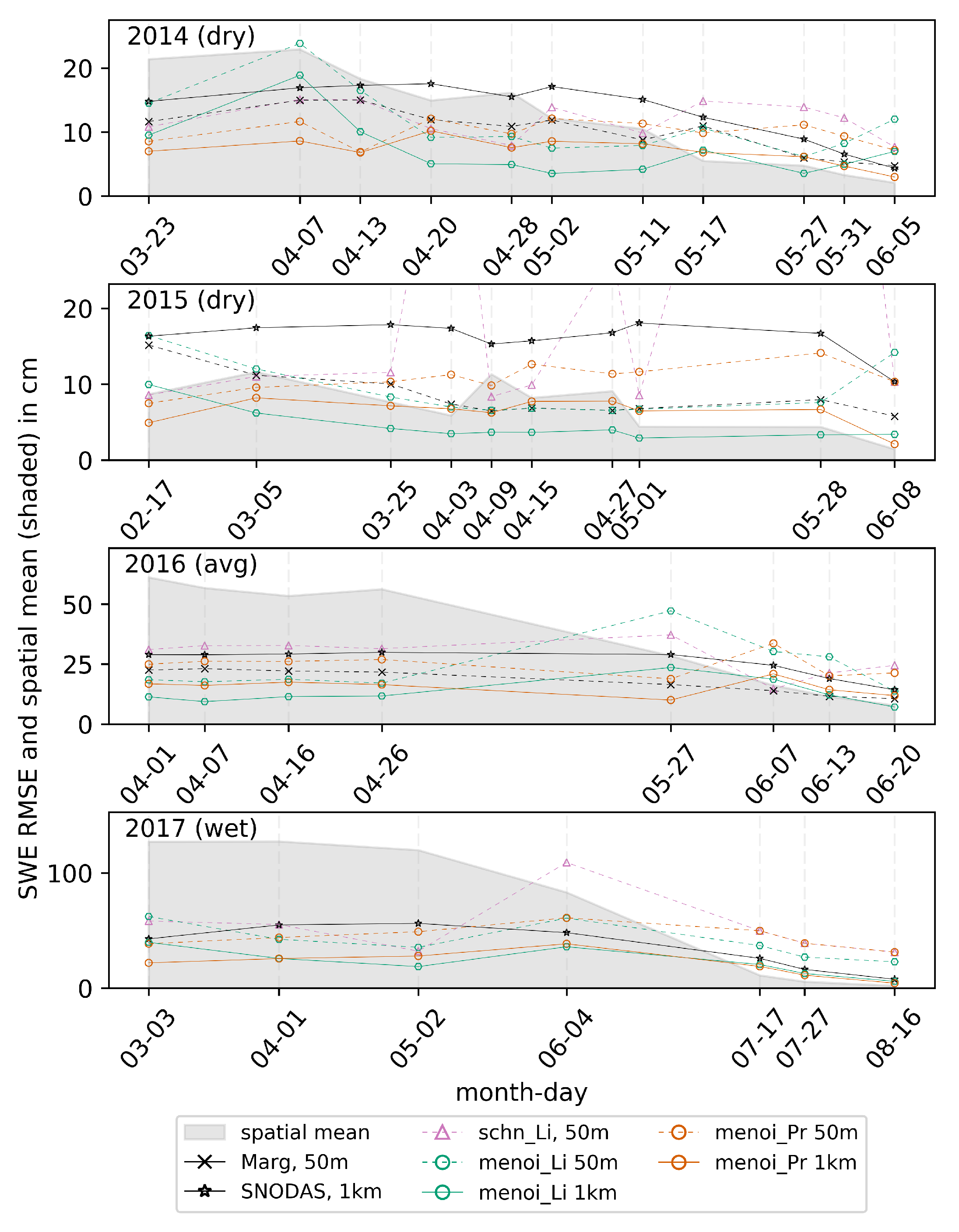
- to what extent does the proposed method based on the Ensemble Optimal Interpolation (EnOI) improve estimation of daily spatial SWE compared to existing methods?
- is it better to use a LiDAR-derived but temporally sparse historical SWE product or a Landsat-derived daily product in the daily SWE estimate?
- How does the proposed method compare to SNODAS, a current operational SWE product?
2. Materials and Methods
2.1. Ensemble Optimal Interpolation (EnOI)
2.2. Prior-Ensemble Sampling
2.3. Experimental Setup
2.4. Dense Historical Samples
2.5. Scarce Historical Samples
2.6. Datasets Summary
- Landsat-derived historical product (90 m SWE):
- Lidar-derived historical product (50 m SWE):
- SNODAS (1 km SWE):
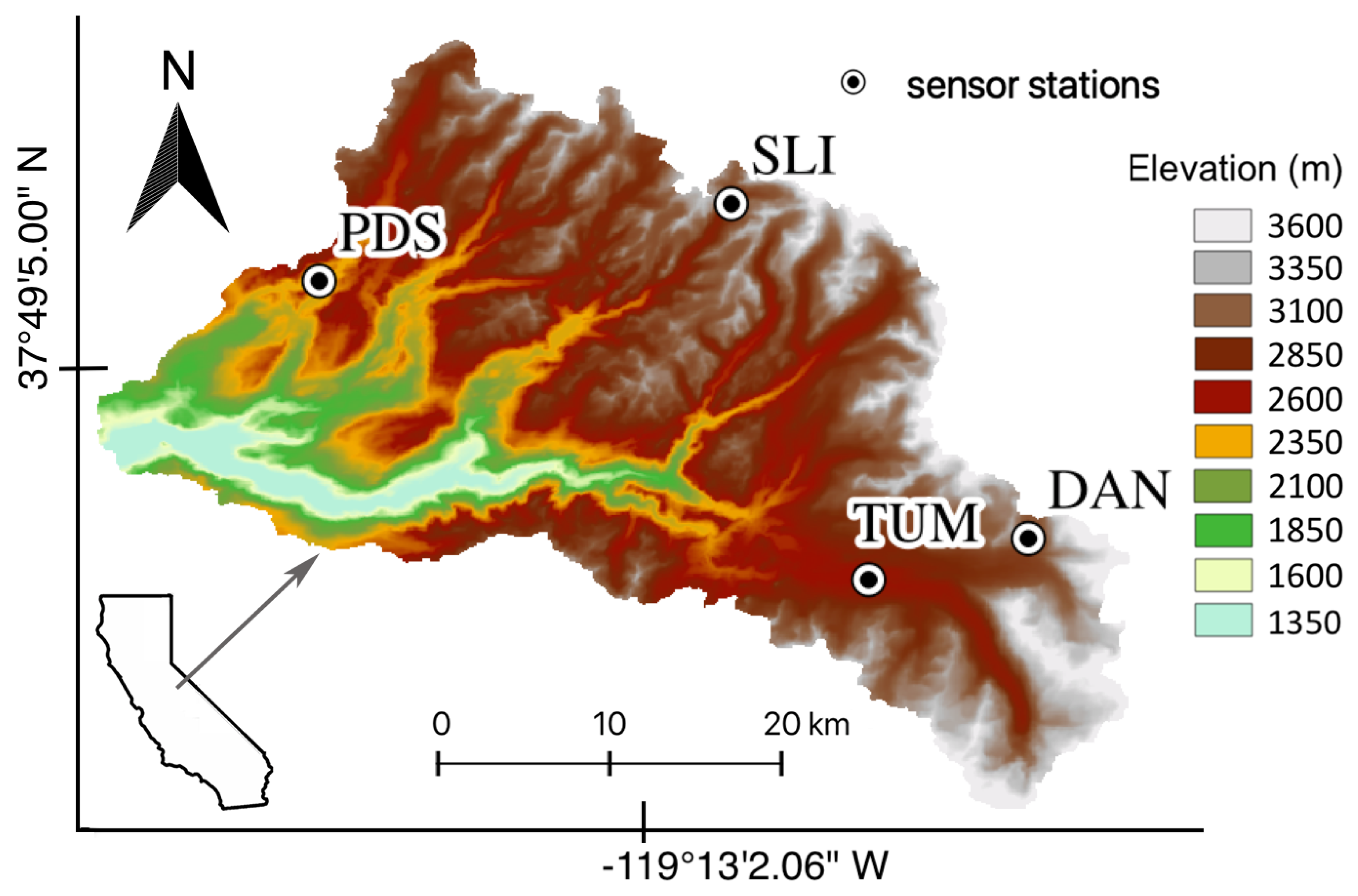
- Sensor locations from CDEC:
- EnOI analysis algorithm:
3. Results
4. Discussion
4.1. Alternative Selections of Prior Ensemble
4.2. LiDAR vs. Satellite-Derived Products
5. Conclusions
Supplementary Materials
Author Contributions
Funding
Conflicts of Interest
References
- Singh, S.; Kumar, R.; Bhardwaj, A.; Sam, L.; Shekhar, M.; Singh, A.; Kumar, R.; Gupta, A. Changing climate and glacio-hydrology in Indian Himalayan Region: A review. WIREs Clim. Chang. 2016, 7, 393–410. [Google Scholar] [CrossRef]
- Lettenmaier, D.P.; Alsdorf, D.; Dozier, J.; Huffman, G.J.; Pan, M.; Wood, E.F. Inroads of remote sensing into hydrologic science during The WRR era. Water Resour. Res. 2015, 51, 7309–7342. [Google Scholar] [CrossRef]
- Kerkez, B.; Glaser, S.D.; Bales, R.C.; Meadows, M.W. Design and Performance of a Wireless Sensor Network for Catchment-scale Snow and Soil Moisture Measurements. Water Resour. Res. 2012, 48, 1–18. [Google Scholar] [CrossRef]
- Rice, R.; Bales, R.C. Embedded-sensor network design for snow cover measurements around snow pillow and snow course sites in The Sierra Nevada of California. Water Resour. Res. 2010, 46. [Google Scholar] [CrossRef]
- Lundquist, J.D.; Cayan, D.R.; Dettinger, M.D. Meteorology and Hydrology in Yosemite National Park: A Sensor Network Application. In Information Processing in Sensor Networks; Zhao, F., Guibas, L., Eds.; Springer: Berlin/Heidelberg, Germany, 2003; pp. 518–528. [Google Scholar]
- Malek, S.A.; Avanzi, F.; Brun-Laguna, K.; Maurer, T.; Oroza, C.A.; Hartsough, P.C.; Watteyne, T.; Glaser, S.D. Real-Time Alpine Measurement System Using Wireless Sensor Networks. Sensors 2017, 17, 2583. [Google Scholar] [CrossRef]
- Dozier, J.; Bair, E.H.; Davis, R.E. Estimating The spatial distribution of snow water equivalent in the world’s mountains. Wiley Interdiscip. Rev. Water 2016, 3, 461–474. [Google Scholar] [CrossRef]
- Girotto, M.; Musselman, K.; Essery, R. Data Assimilation Improves Estimates of Climate-Sensitive Seasonal Snow. Curr. Clim. Chang. Rep. 2020. [Google Scholar] [CrossRef]
- Margulis, S.A.; Cortés, G.; Girotto, M.; Durand, M. A Landsat-Era Sierra Nevada Snow Reanalysis (1985–2015). J. Hydrometeorol. 2016, 17, 1203–1221. [Google Scholar] [CrossRef]
- Kumar, R.; Singh, S.; Kumar, R.; Singh, A.; Bhardwaj, A.; Sam, L.; Randhawa, S.; Gupta, A. Development of a Glacio-hydrological Model for Discharge and Mass Balance Reconstruction. Water Resour. Manag. 2016, 30. [Google Scholar] [CrossRef]
- Cornwell, E.; Molotch, N.P.; McPhee, J. Spatio-temporal variability of snow water equivalent in The extra-tropical Andes Cordillera from distributed energy balance modeling and remotely sensed snow cover. Hydrol. Earth Syst. Sci. 2016, 20, 411–430. [Google Scholar] [CrossRef]
- Rittger, K.; Bair, E.H.; Kahl, A.; Dozier, J. Spatial estimates of snow water equivalent from reconstruction. Adv. Water Resour. 2016, 94, 345–363. [Google Scholar] [CrossRef]
- Liu, M.; Xiong, C.; Pan, J.; Wang, T.; Shi, J.; Wang, N. High-Resolution Reconstruction of The Maximum Snow Water Equivalent Based on Remote Sensing Data in a Mountainous Area. Remote. Sens. 2020, 12, 460. [Google Scholar] [CrossRef]
- Justice, C.O.; Vermote, E.; Townshend, J.R.G.; Defries, R.; Roy, D.P.; Hall, D.K.; Salomonson, V.V.; Privette, J.L.; Riggs, G.; Strahler, A.; et al. The Moderate Resolution Imaging Spectroradiometer (MODIS): Land remote sensing for global change research. IEEE Trans. Geosci. Remote. Sens. 1998, 36, 1228–1249. [Google Scholar] [CrossRef]
- Raleigh, M.S.; Rittger, K.; Moore, C.E.; Henn, B.; Lutz, J.A.; Lundquist, J.D. Ground-based testing of MODIS fractional snow cover in subalpine meadows and forests of The Sierra Nevada. Remote. Sens. Environ. 2013, 128, 44–57. [Google Scholar] [CrossRef]
- Stigter, E.E.; Wanders, N.; Saloranta, T.M.; Shea, J.M.; Bierkens, M.F.P.; Immerzeel, W.W. Assimilation of snow cover and snow depth into a snow model to estimate snow water equivalent and snowmelt runoff in a Himalayan catchment. Cryosphere 2017, 11, 1647–1664. [Google Scholar] [CrossRef]
- Xu, J.; Shu, H. Assimilating MODIS-based albedo and snow cover fraction into the Common Land Model to improve snow depth simulation with direct insertion and deterministic ensemble Kalman filter methods. J. Geophys. Res. Atmos. 2014, 119, 10,684–10,701. [Google Scholar] [CrossRef]
- Sun, C.; Walker, J.P.; Houser, P.R. A methodology for snow data assimilation in a land surface model. J. Geophys. Res. Atmos. 2004, 109. [Google Scholar] [CrossRef]
- Magnusson, J.; Gustafsson, D.; HÃŒsler, F.; Jonas, T. Assimilation of point SWE data into a distributed snow cover model comparing two contrasting methods. Water Resour. Res. 2014, 50, 7816–7835. [Google Scholar] [CrossRef]
- Schneider, D.; Molotch, N.P. Real-time estimation of snow water equivalent in The Upper Colorado River Basin using MODIS-based SWE Reconstructions and SNOTEL data. Water Resour. Res. 2016, 52, 7892–7910. [Google Scholar] [CrossRef]
- Zheng, Z.; Molotch, N.P.; Oroza, C.A.; Conklin, M.H.; Bales, R.C. Spatial snow water equivalent estimation for mountainous areas using wireless-sensor networks and remote-sensing products. Remote. Sens. Environ. 2018, 215, 44–56. [Google Scholar] [CrossRef]
- Erickson, T.A.; Williams, M.W.; Winstral, A. Persistence of topographic controls on The spatial distribution of snow in rugged mountain terrain, Colorado, United States. Water Resour. Res. 2005, 41. [Google Scholar] [CrossRef]
- Deems, J.S.; Fassnacht, S.R.; Elder, K.J. Interannual Consistency in Fractal Snow Depth Patterns at Two Colorado Mountain Sites. J. Hydrometeorol. 2008, 9, 977–988. [Google Scholar] [CrossRef]
- Schirmer, M.; Wirz, V.; Clifton, A.; Lehning, M. Persistence in intra-annual snow depth distribution: 1. Measurements and topographic control. Water Resour. Res. 2011, 47. [Google Scholar] [CrossRef]
- Saavedra, F.A.; Kampf, S.K.; Fassnacht, S.R.; Sibold, J.S. Changes in Andes snow cover from MODIS data, 2000–2016. Cryosphere 2018, 12, 1027–1046. [Google Scholar] [CrossRef]
- Evensen, G. The Ensemble Kalman Filter: Theoretical formulation and practical implementation. Ocean. Dyn. 2003, 53, 343–367. [Google Scholar] [CrossRef]
- Burgers, G.; van Leeuwen, P.J.; Evensen, G. Analysis Scheme in The Ensemble Kalman Filter. Mon. Weather. Rev. 1998, 126, 1719–1724. [Google Scholar] [CrossRef]
- Counillon, F.; Bertino, L. Ensemble Optimal Interpolation: Multivariate properties in The Gulf of Mexico. Tellus A 2009, 61, 296–308. [Google Scholar] [CrossRef]
- Kaurkin, M.N.; Ibrayev, R.A.; Belyaev, K.P. ARGO data assimilation into The ocean dynamics model with high spatial resolution using Ensemble Optimal Interpolation (EnOI). Oceanology 2016, 56, 774–781. [Google Scholar] [CrossRef]
- Fu, W.; Zhu, J. Effects of Sea Level Data Assimilation by Ensemble Optimal Interpolation and 3D Variational Data Assimilation on The Simulation of Variability in a Tropical Pacific Model. J. Atmos. Ocean. Technol. 2011, 28, 1624–1640. [Google Scholar] [CrossRef]
- Evensen, G. Data Assimilation; Springer: Berlin/Heidelberg, Germany, 2009. [Google Scholar]
- Kaurkin, M.N.; Ibrayev, R.A.; Belyaev, K.P. Data assimilation in The ocean circulation model of high spatial resolution using The methods of parallel programming. Russ. Meteorol. Hydrol. 2016, 41, 479–486. [Google Scholar] [CrossRef]
- Painter, T.H.; Berisford, D.F.; Boardman, J.W.; Bormann, K.J.; Deems, J.S.; Gehrke, F.; Hedrick, A.; Joyce, M.; Laidlaw, R.; Marks, D.; et al. The Airborne Snow Observatory: Fusion of Scanning Lidar, Imaging Spectrometer, and Physically-based Modeling for Mapping Snow Water Equivalent and Snow Albedo. Remote. Sens. Environ. 2016, 184, 139–152. [Google Scholar] [CrossRef]
- National Operational Hydrologic Remote Sensing Center. National Operational Hydrologic Remote Sensing Center Snow Data Assimilation System (SNODAS) Data Products at NSIDC; NOHRSC: Minneapolis, MN, USA, 2004.
- Margulis, S.A.; Girotto, M.; Cortés, G.; Durand, M. A Particle Batch Smoother Approach to Snow Water Equivalent Estimation. J. Hydrometeorol. 2015, 16, 1752–1772. [Google Scholar] [CrossRef]
- Conde, V.; Nico, G.; Catalao, J.; Kontu, A.; Gritsevich, M. Wide-area mapping of snow water equivalent by Sentinel-1 & 2 data. In Proceedings of the EGU General Assembly Conference, Vienna, Austria, 23–28 April 2017; p. 9580. [Google Scholar]
- Fassnacht, S.R.; Dressler, K.A.; Bales, R.C. Snow water equivalent interpolation for The Colorado River Basin from snow telemetry (SNOTEL) data. Water Resour. Res. 2003, 39. [Google Scholar] [CrossRef]
- Roche, J.; Bales, R.; Rice, R.; Marks, D. Management Implications of Snowpack Sensitivity to Temperature and Atmospheric Moisture Changes in Yosemite National Park, CA. JAWRA J. Am. Water Resour. Assoc. 2017, 54. [Google Scholar] [CrossRef]
- Howat, I.M.; Tulaczyk, S. Trends in spring snowpack over a half-century of climate warming in California, USA. Ann. Glaciol. 2005, 40, 151–156. [Google Scholar] [CrossRef]
- Schneider, D.; Molotch, N.P.; Deems, J.S. Estimating relationships between snow water equivalent, snow covered area, and topography to extend The Airborne Snow Observatory dataset. Cryosphere Discuss. 2017, 2017, 1–29. [Google Scholar]


| Acronym | Description | Historical Product Used | Features Used | Covariance Sampling | Applied on |
|---|---|---|---|---|---|
| schn | Regression b | LiDAR-derived c | elevation, north-west barrier, south-west barrier, distance-to-ocean, latitude, historical product | N/A | Tuolumne |
| menoi_Li | EnOI | LiDAR-derived | None | all historical samples | Tuolumne |
| menoi_Pr | EnOI | Landsat-derived a | None | all historical samples | Tuolumne |
| SNODAS | SWE from NASA product | N/A | N/A | N/A | Tuolumne |
| marg | Landsat-derived | N/A | N/A | N/A | Tuolumne |
© 2020 by the authors. Licensee MDPI, Basel, Switzerland. This article is an open access article distributed under the terms and conditions of the Creative Commons Attribution (CC BY) license (http://creativecommons.org/licenses/by/4.0/).
Share and Cite
Malek, S.A.; Bales, R.C.; Glaser, S.D. Estimation of Daily Spatial Snow Water Equivalent from Historical Snow Maps and Limited In-Situ Measurements. Hydrology 2020, 7, 46. https://doi.org/10.3390/hydrology7030046
Malek SA, Bales RC, Glaser SD. Estimation of Daily Spatial Snow Water Equivalent from Historical Snow Maps and Limited In-Situ Measurements. Hydrology. 2020; 7(3):46. https://doi.org/10.3390/hydrology7030046
Chicago/Turabian StyleMalek, Sami A., Roger C. Bales, and Steven D. Glaser. 2020. "Estimation of Daily Spatial Snow Water Equivalent from Historical Snow Maps and Limited In-Situ Measurements" Hydrology 7, no. 3: 46. https://doi.org/10.3390/hydrology7030046
APA StyleMalek, S. A., Bales, R. C., & Glaser, S. D. (2020). Estimation of Daily Spatial Snow Water Equivalent from Historical Snow Maps and Limited In-Situ Measurements. Hydrology, 7(3), 46. https://doi.org/10.3390/hydrology7030046