Abstract
Background: The purpose of this work is to discover underlying trends of climate factors, identify their peaks and inflection points between 1880 and 2017, and study their response to climate change. Five climate factors including Land Temperature, Sea Surface Temperature, Temperature Over Land Plus Ocean, Carbon Dioxide concentration, and Northern Hemisphere Sea Ice Extent are studied in this paper. Methods: First, the kernel regression is applied to smooth and recover underlying trends of the climate factors between 1880 and 2017. To characterize temporal changes in the global climate via climate factors, peaks and inflection points of each climate factor are located and identified. Results: Five climate factors are studied between 1880 and 2017. Despite locating multiple inflection points in the climate factors and indicating fluctuations in the weather patterns, it was observed that Land Temperature, Sea Surface Temperature, Temperature Over Land Plus Ocean, and Carbon Dioxide concentration have experienced consistent increasing trends since the mid 20th century. It was also observed that in response to climate change, the Northern Hemisphere Sea Ice Extent has experienced a consistent decreasing trend since the 1960s. Conclusion: An increasing trend was observed for four climate factors (all but Sea Ice Extent) since the early 1900s. Sea Ice Extent shows a consistent decreasing trend dropping to a new minimum, year after year. Among all factors, the Sea Surface Temperature shows a decreasing trend between the late 1800s and the early 1900s. It reaches its minimum in 1911 and has experienced an increasing trend since then. Our observations agree with the global heat content map during this time interval between 1880 and 2017. The heat content in the Americas, Europe, Africa, Asia, and Australia shows an increasing trend since the late 1800s. It agrees with what was observed in the Land Temperature anomalies. In contrast, the heat content of the Pacific, Atlantic, and Indian Oceans shows a decreasing trend from the late 1800s to the early 1900s when its trend turns the course to an increasing trend.
1. Introduction
Global temperature has continued to increase and it has raised concerns about the rapid changes in the global climate system. We are experiencing an increase in the global temperature by 1 degree Celsius since the start of the industrial revolution [1,2,3,4]. This has been the warmest average temperature on Earth since the end of the last Ice Age 12,000 years ago [5]. Global carbon dioxide emissions rose by 1.6% in 2018 and reached a new record high of 37.1 Gigatonnes in comparison with 36.2 Gigatonnes in 2017 [6,7,8,9,10,11]. Northern Hemisphere summer experienced record-breaking heat waves in 2018. Rising levels of greenhouse gases in the atmosphere are increasing the global average temperature and, in turn, they perturb the climate system and increase the frequency and intensity of extreme events, including heat waves, drought conditions, wildfire, and flooding [9,10,11,12,13,14]. Accurate observations and progress in modeling has made it possible to attribute these events to climate change [15]. Global warming causes rising sea levels [16,17,18] because it increases sea surface temperature and it reduces the sea ice extent [19,20]. First, higher sea surface temperature warms the ocean and the ocean takes up more space. Second, reduced sea ice extent causes rising sea levels and hence the ocean takes up more space. The level rise in turn will cause severe coastal erosion that allows higher waves and storm surges to reach the shore. As a result, higher sea surface temperature and reduced sea ice extent affect coastal areas all over the world and increase flooding risk, worsen hurricane damage, and increase migration. The extent of variation in the climate factors can provide information about changes to climate systems. For example, monitoring the sea ice cover is essential for tracking of the ice edge, estimating sea ice concentration, and classifying sea ice types. Passive microwave satellite data represent the best method to monitor sea ice because of the ability to show data through most clouds and during darkness [21]. Collected data by observing polar oceans using passive microwave allows to monitor the variations and trends in sea ice cover for a better understanding of the climate. Satellite data sets reveal considerable regional, seasonal, and annual variability in the ice cover. Discovering the underlying trends in the climate factors is crucial to understand the ramifications of climate change on the living conditions of populations. In our previous works, spatiotemporal mountain glacier variation due to increased temperature was studied using multi-spectral Landsat satellite imagery [22], a monitoring glacier system was proposed using a multiple regression model [23], and a new processed band, normalized difference thermal snow index (NDTSI), was introduced by combining two spectral bands, the so-called B62 and NDSI [24]. In this work, climate change is studied via multiple climate factors including Northern Hemisphere Sea Ice Extent, Land Temperature, Sea Surface Temperature, Temperature Over Land Plus Ocean, and Carbon Dioxide concentration. The underlying trend of each climate factor is estimated using the nonparametric kernel regression method, and trends for different climate factors are compared to discover potential similarities in their temporal patterns since 1880. Moreover, temporal peaks and inflection points are located for each climate factor. Finally, the estimated climate patterns are compared with the global heat content between 1880 and 2017.
2. Methods
The goal is analyzing climate factors to discover underlying changes over the last century, to locate peaks and inflection points, and to find potential temporal correlations of the identified changes among different climate factors. Peaks in each climate factor are identified by locating the zero crossings of the first derivative of the smoothed factor. In a similar way, inflection points are identified by locating the zero crossing of the second derivative of the smoothed factor. A positive (rising) inflection point is a point on the curve where the curve changes from being concave up to be concave down. Whereas a negative (falling) inflection point is a point on the curve where the curve changes from being concave down to be concave up. The Kernel regression, a nonparametric method, is used to smooth the climate factors and characterize the underlying trends. It estimates an underlying function with minimal assumptions regarding the noise model [25,26,27,28]. Let Y be a response variable modeled with regard to a predictor x using . The Kernel regression uses a kernel to calculate a point-wise estimate of nonparametrically. In this work, Y is a climate factor and X is the temporal predictor. The Kernel regression is applied to remove the noise , smooth the climate factor Y, and estimate its temporal trend . After estimating the trend, the peaks of the smoothed climate factor will be located. Peaks are detected by locating the zero crossings of the first derivative of the estimated trend of the climate factor [29]. In a similar way, inflection points are detected by locating the zero crossings of the second derivative of the estimated trend of the climate factor [29]. We have used Tricube kernel for smoothing, because it has finite support to limit the spread of the signal region into local neighboring regions. Tricube has also continuous first, second, and third derivatives within its support and at the boundaries. These characteristics ensure smooth estimates of the function derivatives and reduce edge effects, while facilitating the identification of local peaks and inflection points [22].
3. Data Description
In this paper, we investigated the following climate factors as potential indicators of climate change.
- Land Temperature anomalies
- Sea Surface Temperature anomalies
- Temperature Over Land Plus Ocean
- Carbon Dioxide concentration
- Northern Hemisphere Sea Ice Extent
The climate data are sourced from the National Oceanic and Atmospheric Administration (NOAA) research laboratory, and NASA’s National Snow and Ice Data Center (NSIDC) Distributed Active Archive Center (DAAC). Data for all of these climate factors except sea-ice extent have been collected since 1880 for 138 years from NOAA. The Northern Hemisphere Sea Ice Extent provides a swift look at broad changes in arctic sea-ice and is required for a better understanding of climate. Satellite-borne passive microwave sensors have provided a continuous record of Arctic sea ice extent since 1979. Records before 1979 exist, but the data especially before 1953 are not consistent with the satellite records and have limited reliability [30]. Hence, we study the Sea Ice Extent between 1953 and 2017. NASA launched the Scanning Multichannel Microwave Radiometer (SMMR) in 1978, and the Defense Meteorological Satellite Program (DMSP) launched the first of the Special Sensor Microwave/Imager (SSM/I) sensors in 1987. Scientists at the Goddard Space Flight Center have combined the Scanning Multichannel Microwave Radiometer (SMMR) and the Special Sensor Microwave/Imager (SSM/I) data sets and provided a time series of Sea Ice data that is available from the National Snow and Ice Data Center (NSIDC) from 1979 [31]. Collected data by both SMMR and SSM/I depict annual cycles of ice extent, ice covered area, and variations calculated from the monthly means (Sea Ice anomalies) and are available from NSIDC. Sea Ice Extent records are sourced from Hadley Centre Global Sea Ice and Sea Surface Temperature from 1953 to 1978 [32], and is sourced from NSIDC from 1979 to 2017 [31]. The global heat map frames detailing temperature anomalies from 1880 to 2017 are used for comparison basis ([33]). These color-coded maps display a progression of changing global surface temperature anomalies from 1880 to 2017. Each frame (map) of the image sequence summarizes annual temperature anomalies by averaging temperature anomalies over five years including four preceding years. For example, the image frame for the year 2016 represents averaged global temperature anomalies from 2012 to 2016 (inclusive) in degrees Celsius.
4. Results
In this section, the estimated centennial trends are presented for different climate factors.
4.1. Land Temperature Anomalies
The term temperature anomaly means a departure from a long-term average or reference value. A positive anomaly suggests that the observed temperature was warmer than the reference value, whereas a negative anomaly suggests that the observed temperature was cooler than the reference value. The baseline temperature is generally computed by averaging 30 or more years of temperature data. Peaks and inflection points of the Land Temperature anomalies between 1880 and 2017 (collected by NOAA) are identified. Analysis of the Land Temperature anomalies is performed by smoothing the temporal temperature anomalies and characterizing the trend over the time period between 1880 and 2017 using kernel regression. The maxima and minima of the smoothed signal are then located. As we can see in Figure 1a, only a maximum in 1887 and a minimum in 1892 were identified, and since 1892, the Land Temperature anomalies have been steadily rising. The global heat content concentrations in 1887 (located minimum) and 1892 (located maximum) are shown in Figure 2 for comparison. Figure 1b shows detected inflection points in the smoothed Land Temperature anomalies between 1880 and 2017. Several inflection points in the Land Temperature anomalies are located and are summarized in Table 1. A negative inflection point is identified in 1889 between the located maximum global land temperature in 1887 and the located minimum global land temperature in 1892. In spite of observing several negative and positive inflection points in the Land Temperature anomalies, indicating short term fluctuations during this 138-year period, the overall trend shows a consistent increase of the Land Temperature anomalies since 1892. As we can see in Table 1, the most recent inflection point in the Land Temperature anomalies is in 2010 where a rising inflection point shows increasing temperature.
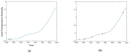
Figure 1.
Land Temperature: (a) Detected maximum (upward green arrow) and minimum (downward green arrow) in the Land Temperature anomalies (Y axis) between 1880 and 2017 (X axis); (b) Identified inflection points in the Land Temperature anomalies (Y axis) between 1880 and 2017 (X axis). Positive inflection point (red diamond); negative inflection point (green diamond).
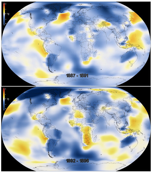
Figure 2.
Global Heat concentrations in 1887 (Top) and 1892 (Bottom).

Table 1.
Positive and negative inflection points of the Land Temperature anomalies.
4.2. Analysis of the Sea Surface Temperature Anomalies
Trends of the Sea Surface Temperature anomalies between 1880 and 2017 are characterized by applying the kernel regression. After recovering the underlying signal, peaks and inflection points are located.
Figure 3a shows the identified peaks in the Sea Surface Temperature between 1880 and 2017. As we can see, there is a single minimum in 1911. There has been a steady increase in the Sea Surface Temperature since 1911. Figure 3b shows detected inflection points in the smoothed Sea Surface Temperature between 1880 and 2017. Several inflection points are located in the Sea Surface Temperature anomalies and are summarized in Table 2. A negative inflection point is detected before 1911 where the Sea Surface Temperature anomalies reach the minimum. Despite identifying a positive inflection point before 1911, the Sea Surface Temperature anomalies have a decreasing trend from 1880 to 1911. Several negative and positive inflection points are identified after 1911. In spite of observing both negative and positive inflection points in the Sea Surface Temperature anomalies after 1911, the overall trend shows a consistent increase of the Sea Surface Temperature anomalies. As we can see in Table 2, the most recent inflection points of the Sea Surface Temperature anomalies are in 2012 and 2013. Similar to the trend of the Land Temperature anomalies, overall trend of the Sea Surface Temperature is indicative of a clear rise since the early 20th century.
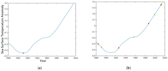
Figure 3.
Sea Surface Temperature: (a) Detected peaks in the Sea Surface Temperature anomalies (Y axis) between 1880 and 2017 (X axis); (b) Identified inflection points in the Sea Surface Temperature anomalies (Y axis) between 1880 and 2017 (X axis). Positive inflection point (red diamond); negative inflection point (green diamond).
Table 2.
Positive and negative inflection points of the Sea Surface Temperature anomalies.
4.3. Analysis of Land and Ocean Anomalies
Next, we studied the Land and Ocean anomalies by recovering the underlying trends between 1880 and 2017 using kernel regression. After characterizing the signal, its peaks and inflection points were detected.
Figure 4a shows a single minimum located in 1905 (between 1880 and 2017). After reaching its minimum in 1905, a steady increase of the Land and Ocean temperature anomalies is observed. Similar to the previous climate factors, i.e., the Land Temperature anomalies and Sea Surface Temperature anomalies, the Land and Ocean Temperature trend demonstrates a clear rise since the early 20th century. Identified inflection points are shown in Figure 4b. As we can see in Table 3, two inflection points are identified before 1905, and four inflection points are located after 1905. The most recent inflection points are in 2010 (positive) and 2011 (negative). Despite identified inflection points that describe the direction of the change, whether it is rising (positive inflection point) or it is falling (negative inflection point), the Land and Ocean Temperature anomalies have been increasing since 1905 and have reached to 0.8 Celsius in 2016.
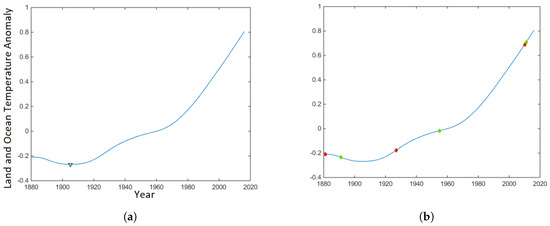
Figure 4.
Land and Ocean Temperature: (a) Detected peaks in the Land and Ocean Temperature anomalies (Y axis) between 1880 and 2017 (X axis); (b) Identified inflection points in the Land and Ocean anomalies (Y axis) between 1880 and 2017 (X axis). Positive inflection point (red diamond); negative inflection point (green diamond).
Table 3.
Positive and negative inflection points of the Land and Ocean anomalies.
4.4. Carbon Dioxide Concentration Anomalies
After smoothing the Carbon Dioxide concentration to recover the underlying CO concentration trend between 1880 and 2017 using kernel regression, a maximum in 1943 and a minimum in 1946 are located (Figure 5a). However, CO concentration has been increasing since 1880. There is just a short time interval between 1943 and 1946 in which it slightly decreased and returned to its increasing trend after the identified minimum in 1946. For comparison bases, global heat content is shown in Figure 6. This figure displays the global heat content in these two time periods where the CO concentration reaches its maximum in 1943 and its minimum in 1946. As we can see, the global heat content is lower (shades of blue) in 1946 (local minimum of CO concentration) in comparison with 1943 (shades of yellow) in which CO concentration reached a local maximum. Figure 6 shows that the global heat index has the same trend and has been decreasing over the time period between 1943 and 1946.
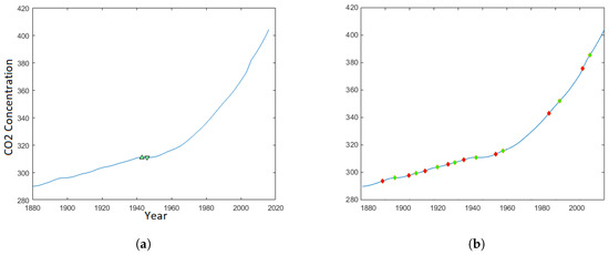
Figure 5.
CO2 concentration: (a) Detected maximum (upward green arrow) and minimum (downward green arrow) in CO2 concentration (Y axis) between 1880 and 2017 (X axis); (b) Identified inflection points in CO2 concentration (Y axis) between 1880 and 2017 (X axis). Positive inflection point (red diamond); negative inflection point (green diamond).
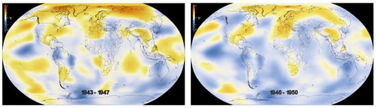
Figure 6.
Heat content: in 1943 where CO had a local maximum (Left); in 1946 where CO had a local minimum (Right). The temperature anomalies are represented within a range from -2 degrees Celsius (dark blue) to +2 degrees Celsius (dark orange).
Identified inflection points in CO concentration are shown in Figure 5b. Detected positive and negative inflection points are summarized in Table 4. As we can see, there is a rising inflection point located in 1937 before reaching the local maximum (in 1943) and a negative inflection point in 1944 after reaching the local maximum. Similarly, the falling inflection point located in 1944 is before the local minimum (in 1946) and a rising inflection point in 1955 is after reaching the local minimum. Six inflection points are identified in CO concentration after reaching a local minimum in 1946. Despite locating both negative and positive inflection points between 1946 and 2017, the general trend of CO concentration have been consistently increasing and reached 400 ppm in 2016. Several negative and positive inflection points in CO concentration indicate fluctuations in weather patterns during this time interval.
Table 4.
Positive and negative inflection points of CO concentration between 1880 and 2017.
4.5. Northern Hemisphere Sea Ice Extent
The last factor that is investigated is the Northern Hemisphere Sea Ice and Snow Cover Extent. It has experienced substantial changes (Figure 7) in past decades.
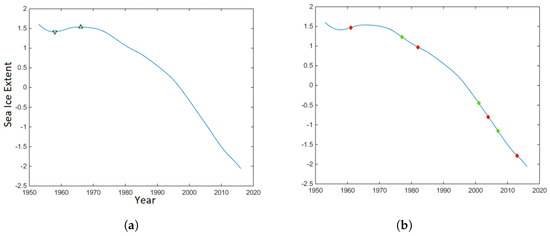
Figure 7.
Northern Hemisphere Sea Ice Extent: (a) Detected peaks of Sea Ice Extent (Y axis) between 1953 and 2017 (X axis); (b) Identified inflection points of Sea Ice Extent (Y axis) between 1953 and 2017 (X axis). Positive inflection point (red diamond); negative inflection point (green diamond).
Peaks and inflection points are then located in the smoothed Sea Ice Extent between 1953 and 2017 (Figure 7). Positive and negative inflection points are summarized in Table 5. A weak local minimum in 1958 and a local maximum in 1966 are located (Figure 7a). After reaching to its identified maximum in 1966, a steady decrease in the annual average Sea Ice Extent is observed. Identified inflection points are depicted in Figure 7b. There is a positive inflection point in 1961 before Sea Ice Extent reached its maximum in 1966. Despite five identified inflection points after reaching its maximum, Sea Ice Extent has a steady response to the changing climate and it has been consistently decreasing (Table 5). Similar to the other climate factors that are studied in this research, Sea Ice Extent shows consistent trend in response to climate change.
Table 5.
Positive and negative inflection points of Sea Ice Extent between 1953 and 2017.
5. Summary and Discussion
Five climate factors, including Land Temperature, Sea Surface Temperature, Temperature Over Land Plus Ocean, Carbon Dioxide concentration, and Northern Hemisphere Sea Ice Extent, were studied between 1880 and 2017 (from 1953 to 2017 for Sea Ice Extent) in this paper. To recover underlying trends for each factor, the kernel regression was used. After smoothing the climate factors, the peaks and inflection points of each factor were located where an infection point is the point that the direction of climate factor variation will switch from increasing change to decreasing change or vice versa.
A local minimum was located in each of Land, Sea Surface, and Land Plus Ocean Temperatures in the late 1800s or the early 1900s. Despite having multiple inflection points, all three factors demonstrate a consistent increase after reaching their minima, which reveals that the factors have been reaching new higher levels over the past century. The Carbon Dioxide concentration shows an increasing trend since the late 1800s. In its increasing trend, the Carbon Dioxide concentration experienced an insubstantial local minimum in 1946 and returned back to its increasing trend right after. Identified inflection points after the Carbon Dioxide reached its local minimum indicate short-term fluctuations in Carbon Dioxide concentration. The most recent inflection point in its concentration is in 2008. In contrast with the other four factors, the Sea Ice Extent has experienced a consistent decreasing trend since the mid 1900s. In its decreasing trend, it experienced a weak local maximum in 1966 and gets back to its decreasing trend afterward.
The identified features of all studied climate factors demonstrate a warmer climate with an upward trend since the early 1900s. Our observations agree with the global heat content map detailing temperature anomalies since 1880. As we can observe in Figure 8, the heat content in the Americas, Europe, Africa, Asia, and Australia shows an increasing trend since the late 1800s, similar to what we observed in Land Temperature anomalies. In contrast, the heat content of the Pacific, Atlantic, and Indian Oceans shows a decreasing trend from the late 1800s to the early 1900s and then its trend turns the course to increasing. This agrees with our observations of the Sea Surface Temperature anomalies. As we can see from the global temperature anomalies in Figure 8, the global heat content is saturating and has increased over one degree Celsius demonstrated in yellow, orange, and red, while almost no shades of blue can be seen.
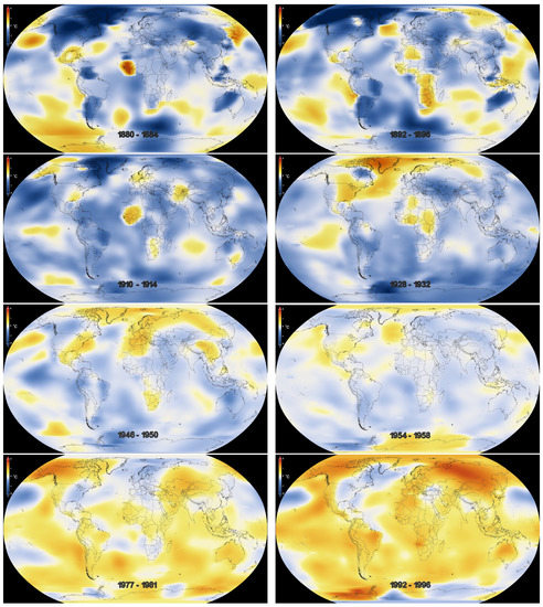
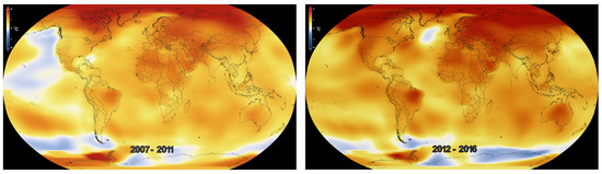
Figure 8.
Global heat content between 1880 and 2017. The temperature anomalies are represented within a range from -2 degrees Celsius (dark blue) to +2 degrees Celsius (dark orange).
A centennial increasing trend of Sea Surface temperature and multi-decadal decreasing trend of Sea Ice Extent were observed, which have potentially been the deriving forces of increasing sea level. An increasing trend of sea level will potentially cause an increasing trend of coastal erosion that, in turn, will cause higher waves and storm surges to reach the shore. As a result, sea level rise can potentially increase the flooding risk and worsen the damages on coastal areas all over the world.
We should point out that, identifying the inflection points in climate variables is essential to discover the spatiotemporal non-climate factors, such as economic, industrial, energy consumption, and public health factors, that could potentially be associated with the peak or curvature change of climate factors and in turn may have contributed to climate change. The main objective of this research was to study the climate factors in association with climate change. Follow-up research is encouraged by this work to study potential non-climate factors in association with identified temporal climate factor features.
Author Contributions
Formal analysis, N.N.K. and O.E.O.; Investigation, N.N.K. and O.E.O.; Methodology, N.N.K.; Project administration, N.N.K.; Visualization, N.N.K. and O.E.O.; Writing–original draft, N.N.K. and O.E.O.; Writing–review and editing, N.N.K. and O.E.O. All authors have read and agree to the published version of the manuscript.
Funding
Publication of this article was funded in part by the Open Access Subvention Fund and the John H. Evans Library.
Acknowledgments
NOAA Global Surface Temperature (NOAAGlobalTemp) data provided by the NOAA/OAR/ ESRL PSD, Boulder, Colorado, USA, from their Web site at https://www.esrl.noaa.gov/psd/.
Conflicts of Interest
The authors declare no conflict of interest.
References
- Kraaijenbrink, P.; Bierkens, M.; Lutz, A.; Immerzeel, W. Impact of a global temperature rise of 1.5 degrees Celsius on Asia’s glaciers. Nature 2017, 549, 257–260. [Google Scholar] [CrossRef] [PubMed]
- Clark, P.U.; Mix, A.C.; Eby, M.; Levermann, A.; Rogelj, J.; Nauels, A.; Wrathall, D.J. Sea-level commitment as a gauge for climate policy. Nat. Clim. Chang. 2018, 8, 653–655. [Google Scholar] [CrossRef]
- Rasmussen, D.; Bittermann, K.; Buchanan, M.K.; Kulp, S.; Strauss, B.H.; Kopp, R.E.; Oppenheimer, M. Extreme sea level implications of 1.5 C, 2.0 C, and 2.5 C temperature stabilization targets in the 21st and 22nd centuries. Environ. Res. Lett. 2018, 13, 034040. [Google Scholar] [CrossRef]
- FutureEarth. 10 New Insights in Climate Science 2018. Available online: https://futureearth.org/publications/science-insights/10-new-insights-in-climate-science-2019/ (accessed on 5 March 2019).
- King, A.D. Attributing changing rates of temperature record breaking to anthropogenic influences. Earth Future 2017, 5, 1156–1168. [Google Scholar] [CrossRef]
- Levin, K. New Global CO2 Emissions Numbers Are In. 2018. Available online: https://www.wri.org/blog/2018/12/new-global-co2-emissions-numbers-are-they-re-not-good (accessed on 5 March 2019).
- Smith, P.; Davis, S.J.; Creutzig, F.; Fuss, S.; Minx, J.; Gabrielle, B.; Kato, E.; Jackson, R.B.; Cowie, A.; Kriegler, E.; et al. Biophysical and economic limits to negative CO2 emissions. Nat. Clim. Chang. 2016, 6, 42–50. [Google Scholar] [CrossRef]
- Muller, D.B.; Liu, G.; Løvik, A.N.; Modaresi, R.; Pauliuk, S.; Steinhoff, F.S.; Brattebø, H. Carbon emissions of infrastructure development. Environ. Sci. Technol. 2013, 47, 11739–11746. [Google Scholar] [CrossRef]
- Panagoulia, D.; Dimou, G. Sensitivity of flood events to global climate change. J. Hydrol. 1997, 191, 208–222. [Google Scholar] [CrossRef]
- Holland, G.; Bruyère, C.L. Recent intense hurricane response to global climate change. Clim. Dyn. 2014, 42, 617–627. [Google Scholar] [CrossRef]
- Trenberth, K.E.; Cheng, L.; Jacobs, P.; Zhang, Y.; Fasullo, J. Hurricane Harvey links to ocean heat content and climate change adaptation. Earth Future 2018, 6, 730–744. [Google Scholar] [CrossRef]
- Patricola, C.M.; Wehner, M.F. Anthropogenic influences on major tropical cyclone events. Nature 2018, 563, 339–346. [Google Scholar] [CrossRef]
- Dosio, A.; Mentaschi, L.; Fischer, E.M.; Wyser, K. Extreme heat waves under 1.5 C and 2 C global warming. Environ. Res. Lett. 2018, 13, 054006. [Google Scholar] [CrossRef]
- Schiermeier, Q. Droughts, heatwaves and floods: How to tell when climate change is to blame. Nature 2018, 560, 20–22. [Google Scholar] [CrossRef] [PubMed]
- Gutmann, E.D.; Rasmussen, R.M.; Liu, C.; Ikeda, K.; Bruyere, C.L.; Done, J.M.; Garrè, L.; Friis-Hansen, P.; Veldore, V. Changes in hurricanes from a 13-yr convection-permitting pseudo–global warming simulation. J. Clim. 2018, 31, 3643–3657. [Google Scholar] [CrossRef]
- Mimura, N. Sea-level rise caused by climate change and its implications for society. Proc. Jpn. Acad. Ser. 2013, 89, 281–301. [Google Scholar] [CrossRef] [PubMed]
- ClimateGov. Sea Level Rise Since 1880, /Climate-Change-Global-Sea-Level. 2019. Available online: http://xxx.lanl.gov/abs/https://www.climate.gov/news-features/understanding-climate (accessed on 5 March 2019).
- Kulp, S.A.; Strauss, B.H. New elevation data triple estimates of global vulnerability to sea-level rise and coastal flooding. Nat. Commun. 2019, 10, 1–12. [Google Scholar]
- ClimateGov. Arctic Sea Ice Minimum in 2017, /2017-Arctic-Sea-Ice-Minimum-Comes-Eighth-Smallest- Record. 2017. Available online: http://xxx.lanl.gov/abs/https://www.climate.gov/news-features/featured-images (accessed on 10 June 2018).
- ClimateGov. Old Thick Ice Barely Survives Today’s Arctic in 2019, /2019-Arctic-Report-Card-Old- Thick-Ice-Barely-Survives-Today’s-Arctic. 2019. Available online: http://xxx.lanl.gov/abs/https://www.climate.gov/news-features/featured-images (accessed on 5 March 2019).
- NSIDC. Sea Ice. 2019. Available online: http://xxx.lanl.gov/abs/https://nsidc.org/cryosphere/sotc/sea_ice.html (accessed on 5 March 2019).
- Kachouie, N.N.; Gerke, T.; Huybers, P.; Schwartzman, A. Nonparametric regression for estimation of spatiotemporal mountain glacier retreat from satellite images. IEEE Trans. Geosci. Remote. Sens. 2014, 53, 1135–1149. [Google Scholar] [CrossRef]
- Onyejekwe, O.; Holman, B.; Kachouie, N.N. Multivariate models for predicting glacier termini. Environ. Earth Sci. 2017, 76, 807. [Google Scholar] [CrossRef]
- Kachouie, N.N.; Huybers, P.; Schwartzman, A. Localization of mountain glacier termini in Landsat multi-spectral images. Pattern Recognit. Lett. 2013, 34, 94–106. [Google Scholar] [CrossRef]
- Takeda, H.; Farsiu, S.; Milanfar, P. Kernel Regression for Image Processing and Reconstruction. IEEE Trans. Image Process. 2007, 16, 349–366. [Google Scholar] [CrossRef]
- Lin, E.B.; Ling, Y. Image Compression and Denoising via Nonseparable Wavelet Approximation. J. Comput. Appl. Math. 2003, 155, 131–152. [Google Scholar] [CrossRef]
- Wasserman, L. All of Nonparametric Statistics, 1st ed.; Springer Publishing Company, Incorporated: Berlin/Heidelberg, Germany, 2010. [Google Scholar]
- Rencher, A. Methods of Multivariate Analysis; Wiley Series in Probability and Statistics; Wiley: Hoboken, NJ, USA, 2003. [Google Scholar]
- Kachouie, N.N.; Lin, X.; Schwartzman, A. FDR control of detected regions by multiscale matched filtering. Commun. Stat. Simul. Comput. 2017, 46, 127–144. [Google Scholar] [CrossRef] [PubMed]
- Pirón, M.A.C.; Pasalodos, J.A.C. Nueva serie de extension del hielo marino ártico en septiembre entre 1935 y 2014. Rev. Climatol. 2016, 16, 1–19. [Google Scholar]
- NSIDC. National Snow and Ice Data Center. 2019. Available online: http://xxx.lanl.gov/abs/https://nsidc.org/data (accessed on 5 March 2019).
- Met Office Hadley Centre Observations Datasets. HadISST1 Data. Available online: https://www.metoffice.gov.uk/hadobs/hadisst/ (accessed on 5 March 2019).
- NASA. Five-Year Global Temperature Anomalies from 1880 to 2016, 2017. Available online: http://xxx.lanl.gov/abs/https://nsidc.org/data (accessed on 10 June 2018).


© 2020 by the authors. Licensee MDPI, Basel, Switzerland. This article is an open access article distributed under the terms and conditions of the Creative Commons Attribution (CC BY) license (http://creativecommons.org/licenses/by/4.0/).