Article

Evaluation of General Circulation Models over the Upper Ouémé River Basin in the Republic of Benin

by
André Attogouinon
1,*,
Agnidé E. Lawin
2 and
Jean-François Deliège
3
1
International Chair in Mathematical Physics and Applications (ICMPA—UNESCO CHAIR), University of Abomey-Calavi, Cotonou 072 Po Box 50, Benin
2
Laboratory of Applied Hydrology, National Institute of Water, University of Abomey-Calavi, Cotonou 01 Po Box 4521, Benin
3
Aquapole, PeGIRE R&D Unit, FOCUS Unit Research, University of Liege, Campus du Sart Tilman, B53, Quartier Polytech 1, Allee de la découverte, 11, B-4000 Liege, Belgium
*
Author to whom correspondence should be addressed.
Hydrology 2020, 7(1), 11; https://doi.org/10.3390/hydrology7010011
Submission received: 28 November 2019 / Revised: 28 January 2020 / Accepted: 4 February 2020 / Published: 14 February 2020

Abstract

:
This study assessed the performance of eight general circulation models (GCMs) implemented in the upper Ouémé River basin in Benin Republic (West Africa) during the Fifth Assessment Report on Climate Change. Historical rainfall simulations of the climate model of Rossby Regional Centre (RCA4) driven by eight Coupled Model Intercomparison Project (CMIP5) GCMs over a 55-year period (1951 to 2005) are evaluated using the observational data set. Apart from daily rainfall, other rainfall parameters calculated from observed and simulated rainfall were compared. U-test and other statistical criteria (R2, MBE, MAE, RMSE and standard of standard deviations) were used. According to the results, the simulations correctly reproduce the interannual variability of precipitation in the upper Ouémé River basin. However, the models tend to produce drizzle. Especially, the overestimation of April, May and November rains not only explains the overestimation of seasonal and annual cumulative rainfall but also the early onset of the rainy season and its late withdrawal. However, we noted that this overestimation magnitude varies from one model to another. As for extreme rainfall indices, the models reproduced them poorly. The CanESM2, CNRM-CM5 and EC-EARTH models perform well for daily rainfall. A trade-off is formulated to select the common MPI-ESM-LR, GFDL-ESM2M, NorESM1-M and CanESM2 models for different rainfall parameters for the reliable projection of rainfall in the area. However, the MPI-ESM-LR model is a valuable tool for studying future climate change.

1. Introduction

Climate change resulting from anthropogenic greenhouse gas (GHG) emissions has adverse impacts on human lives, properties and the environment. Humans can only protect themselves from the inherent damage and manage the consequences of climate change by thinking about the development of projections of future changes. General circulation models (GCMs) are the most reliable means of estimating future climate change in an atmosphere where the concentration of greenhouse gases continues to increase significantly [1,2,3]. A climate model can be used to simulate past or future climate (climate projection). In addition to empirical laws and statistical adjustments, a climate model is based on fundamental physical laws (i.e., principles of conservation of mass, energy and moments) that can be mathematically transcribed [4]. Because of the large number of processes and interactions between the atmosphere, ocean and biosphere, the climate model is extremely complex. However, this sophisticated tool is limited by the computing power and time available today [5]. Thus, it does not allow taking into account fine-scale physical processes (e.g., local convection that determines point precipitation), which are necessary for a good representation of the local climate. To overcome this major drawback, researchers have developed regional climate models (RCMs). These models are applied in a limited area domain with lateral boundary conditions (LBCs) provided by a global climate model or reanalysis. The high-resolution RCM therefore simulates small-scale features from lower-resolution boundary information [6]. This allows the addition of small-scale information related to climate change projections [7]. However, the results of these climate models remain dependent on fairly large uncertainties [8,9]. In Africa, climate models are relatively satisfactory in predicting temperature changes. On the other hand, uncertainties remain on the results of rainfall projections. Giannini [10] has shown that there is a significant disagreement between GCMs on the future evolution of rainfall in West Africa [11,12]. In the IPCC report, no conclusions are drawn regarding the rainfall regime in West Africa. Climate projections of rainfall are therefore still uncertain for West Africa. However, West Africa is one of the most vulnerable regions of the continent, often subject to the adverse effects of climate change [13,14]. It is therefore essential to evaluate climate simulation tools in West Africa, especially considering that rainfall forecasts are of major importance for most vulnerabilities, mitigation and adaptation. In Benin, better rainfall forecasting is needed in the upper Ouémé River basin for better decision-making. Indeed, the upper Ouémé River basin is an important agricultural reservoir for the country where agriculture is the main source of economic wealth creation. Moreover, it is located at the foot of Mount Tanéka in the commune of Copargo where the source of the Ouémé River is located, whose floods cause catastrophic flooding in most of the southern regions of the country. The main objective of our research is to verify whether the climate model of the Rossby Regional Centre (RCA4) is capable of representing the main past characteristics of the medium climate and its variability over the period 1951–2005. Particular attention is paid to precipitation. The evaluation of the RCA4 regional model involves the statistical comparison of certain rainfall parameters over the upper Ouémé River basin. Therefore, the RCA4 simulations driven by certain CMIP5 GCMs with a resolution between 100 and 300 km [15] are compared with observations, which makes it possible to estimate the biases or deviations of the GCMs. This research has several advantages. The interest and motivation to carry out this study are related to several aspects. First of all, the subject is part of a CORDEX (COordinated Regional Climate Downscaling EXperiment) scientific research context. The main objectives are to better understand regional and local climate phenomena, not only to evaluate models but also to improve scaling techniques [16]. Then, in the more or less long term, the results of the study can be used as a tool for planners and decision makers and to predict the impact of climate change risks on human activities and ecosystems in order to improve response capacities.

2. Materials and Methods

2.1. Study Site

Benin is a West African country with estimated population of 9,983,884 inhabitants [16], located (Figure 1) between longitudes 1° E and 3°40′ E and latitudes 6°30′ N and 12°30′ N. It is bordered by the Atlantic Ocean in the south, the Federal Republic of Nigeria in the east, Togo in the west, Burkina Faso in northwest and Niger in the north. The only high mountain chain is no more than 600 m in elevation and is located in western north of the country. The climate is characterized by a bimodal precipitation regime in the south and unimodal rainfall regime in the north while the central part of the country is under a transitional precipitation regime. The mean maximum temperature for the whole country varies between 28 and 33.5 °C, while the mean minimum temperature fluctuates between 24.5 and 27.5 °C. In the southern part of the country, the mean annual precipitation varies from 1500 mm in the east to 900 mm in the west, while in the northern region it varies from 700 mm in the far north to 1200 mm in the middle north. The main important rivers are Mékrou, Alibori and Sota in the north, and Ouémé (the major river of the country), Mono and Couffo in the middle and southern parts of the country.
The upper Ouémé River basin, which is the study area, is located between 9° N and 10° N latitude and 1.5° E and 2.8° E longitude. The climate is characterized by the alternation of a unique rainy season and a dry season of approximately equivalent duration. The dry period ranges from November to March. All the rivers of this basin are characterized by an intermittent regime.
The mesoscale site of the upper Ouémé River basin (Benin) is part of the network of mesoscale observation sites of the AMMA-CATCH observatory. Thus, the upper Ouémé River basin is one of the most instrumented regions in West Africa. Different instruments are deployed there to monitor the water cycle and vegetation dynamics.

2.2. Observational Data

In this research, rainfall series for “essential factor of differentiation in tropical environment” [17,18] have been used. A network of eight stations out of the twenty of the rainfall networks managed by the Benin Meteo Agency (Figure 1), given the length of their series, missing data and aspects of temporal homogeneity, have been exploited. The stations having at least data on the period 1951–2005 and less than 20% missing rainy season data [19] were selected. The complete list of these stations and their geographical coordinates are presented in Table 1. The stations of Kouandé and Tchaourou do not belong directly to our study site but have an influence on it.

2.3. Models

We evaluated a set of CMIP5 GCM-driven RCM simulations over West Africa. The RCM simulation outputs used here result from dynamic downscaling of eight CMIP5 GCMs’ data using the RCA4, originally developed by the Swedish Meteorological and Hydrological Institute (SMHI) as part of the CORDEX initiative. Simulated outputs from RCA4 are available over Africa at a spatial resolution of 0.44° × 0.44° (~50 × 50 km) with temporal coverage from 1951 to 2005 in the Coordinated Regional Climate Downscaling Experiment (CORDEX) program context. Only historical simulations were used in this study. The resulting outputs from the eight CMIP5 models’ data, dynamically downscaled by RCA4 during the fifth report on climate change (AR5) were obtained on the research website (http://www.cordex.org/data-access/esgf/). A single ensemble run was performed for each model, although some models had multiple ensemble runs. The set used was r1i1p1. In this research, we considered GCMs that simulate data for each of the 365 days of each year. However, the HadGEM2-ES model, which simulates data for only 360 days out of 365 of each year, was also considered and the missing data were generated using the R package forecast language. Table 2 provides details of the GCMs’ data used in the downscaling experiment.

2.4. Model Performance

The analysis of the performance of the models with respect to the climatic observations needs a comparison between the observed values and those simulated by the climate models under consideration. Thus, observed and simulated daily rainfalls were compared. However, the annual, seasonal, quarterly and monthly totals as well as the moving averages calculated from these observed and simulated daily precipitations were also compared. To make the analysis much more complete, the rainfall indices (Table 3) were calculated from the observed data and those simulated by the models. These indices were then compared.
Statistical criteria were used to compare the simulated against the observed data. It is recommended to use the mean absolute error (MAE) in model evaluation studies [20,21]. However, the root-mean-square error (RMSE) is more appropriate to represent model performance than the MAE when the error distribution should be Gaussian [22], and the use of RMSE is beneficial in certain circumstances. However, these authors recognize that when evaluating different models using a single metric, the differences in error distributions become larger. Accordingly, a combination of measures including (but certainly not limited to) RMSE and MAE is often necessary to evaluate model performance. In the present research, we used U-test [23] and statistical criteria such as the Pearson correlation coefficient calculation [3], the deviations of the standard deviations [3,24] as well as the mean bias (MBE) calculation [19], the MAE [19,20,22] and the RMSE for the comparison between simulated and observed daily rainfall; for the precipitation indices, annual, seasonal, quarterly and monthly total rainfall, MBE, MAE and RSME were used. The choice of these different criteria mentioned above for the evaluation of the results of the models is based on the fact that each criterion helps to appreciate a certain performance of the models. The procedure for the evaluation of GCMs based on their historical simulation of precipitation is outlined below:
  • The use of U-test will help to assess whether the numerical general circulation models (GCMs) are sufficiently reliable.
  • The correlation is used to quantify the linear relationship between observed rainfall and those simulated by the models. The calculation of the Pearson correlation coefficient is based on the calculation of the covariance between the two variables. The correlation coefficient is actually the standardization of the covariance.
  • The difference between the standard deviations of observed rainfall and those simulated by the models provides information on the simulation of interannual variability by the models.
  • MBE makes it possible to quantify the average systematic error (mean bias) of each model. The better the accuracy of the estimation model, the lower the mean bias. A positive bias indicates a tendency to overestimate the model, conversely a negative bias indicates that the estimated values are underestimated compared to those actually observed. The average bias (MBE) is calculated from the following formula:
    M B E = j = 1 M [ i = 1 N ( X S i m   i , j X O b s   i , j ) N ] M
    where X is the value of the parameter considered for each year (period from April to October) for the period of 55 years (1951–2005); Obs corresponds to observations and Sim to simulations. N is the number of years (i.e., 55 years) and M is the number of stations considered for each model on our study site.
  • MAE allows to quantify the amplitude of the average errors regardless of the positive or negative biases (magnitude of the differences between the simulated and observed values). The mean absolute error (MAE) is defined as follows:
    M A E = j = 1 M [ i = 1 N | X S i m   i , j X O b s   i , j | N ] M
  • RMSE allows to include evidence of not only the errors in the mean value but also those in the interannual variability of the simulated versus observed data. If the RMSE is almost identical to the mean absolute error (and not zero), a systematic error affects the mean value of the simulated values and the error on the variability is therefore low or zero. On the other hand, if the RMSE is greater than the MAE (and not zero), the simulated values are affected both by an error in the mean value of the data but also by an error in the interannual variability. RMSE is often used to describe the dispersion of observations and simulations (the lower the RMSE is, the more that the prediction models are related the observations). The RMSE is calculated according to the following formula:
    R M S E = j = 1 M i = 1 N ( X S i m   i , j X O b s   i , j ) 2 N M
    Statistical analyses were performed using the statistical software R 3.5.1 (R Development Core Team, http://www.R-project.org) with packages stats and forecast.

3. Results

3.1. U-Test Results

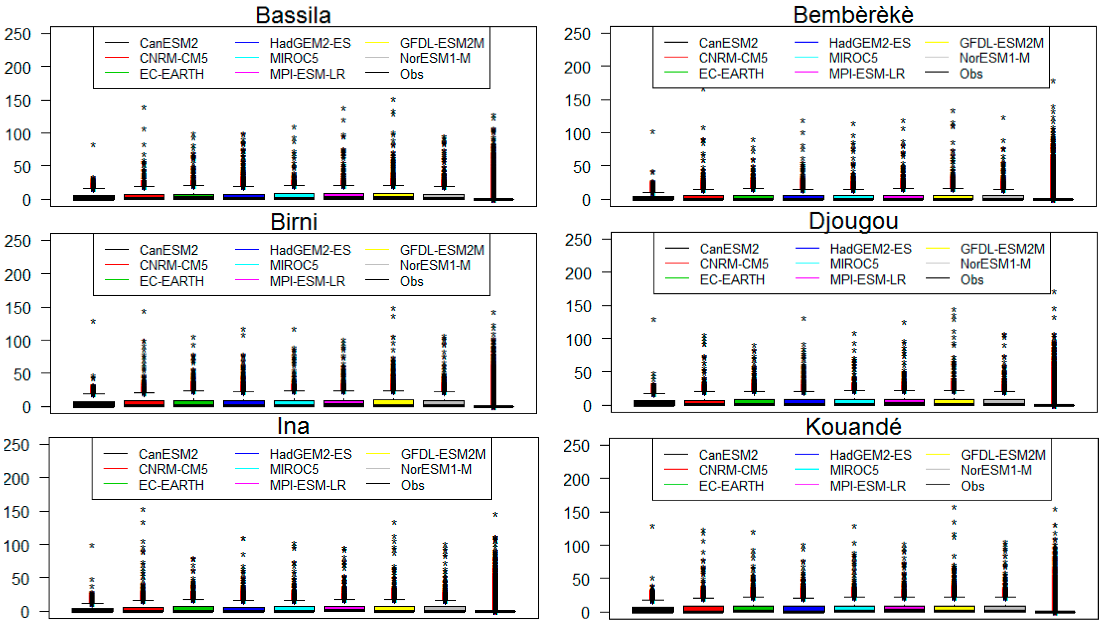
First, the U-test or rank test (that tests the equality of two distributions) was performed, in order to assess the temporal reproduction of precipitation by the models. For this test, p-value took the value 2.2 × 10 6 in all stations. The results of this test showed that there was a significant difference between the simulated and observed data at the 5% level at the eight stations. The boxplot of observed and simulated data (Figure 2) clearly shows that the models tend to produce drizzle (overestimate low precipitation and underestimate heavy rainfall). Indeed, the heavy rains simulated by the models are much more concentrated between 20 and 50 mm. Observed rainfall above 50 mm is well taken into account by the models. This is much more evident with the model CanESM2.
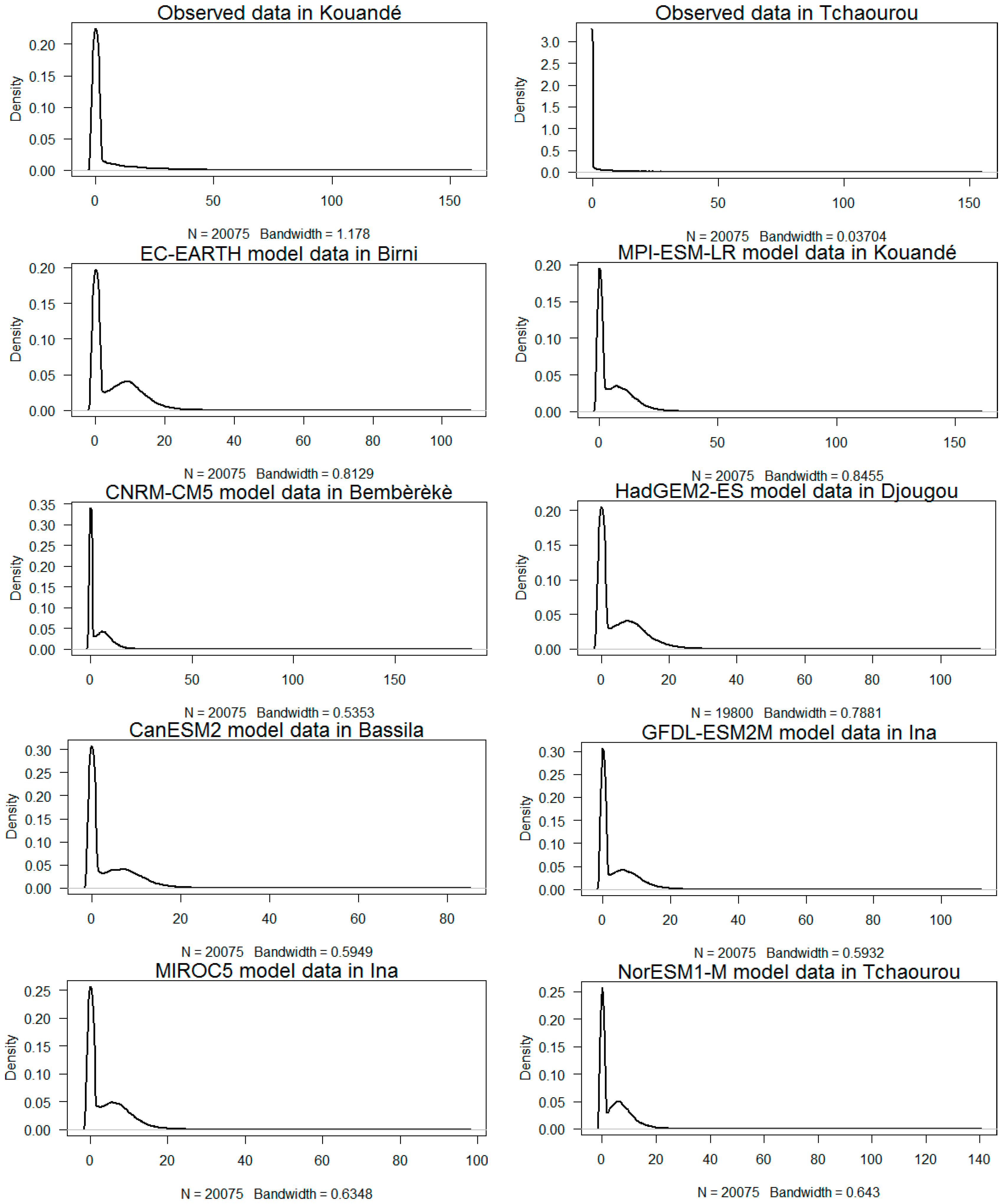
The estimated rainfall values between 0 and 20 mm have a high density (Figure 3), which shows a natural tendency of climate models to estimate rainfall levels much lower than those observed in the field. In other words, the models predict more rainy days than observed. Extreme values are less predictable. In the figure below, we have, on the abscissa, the rainfall height expressed in millimeters (mm).

3.2. Correlation Test Results

Table 4 below gives the values of the correlation coefficient for all stations between observed and simulated rainfall values. Table 4 shows a weak correlation between the observed and the simulated values. Indeed, according to this table, it is observed that the correlation coefficients are low for all the stations. They are positive for all models except for the model HadGEM2-ES, where they are particularly weaker and negative at all stations. The correlation coefficients are higher for the model CNRM-CM5.

3.3. Interannual Variability

The simulated interannual rainfall variability of all stations studied is underestimated. Indeed, the deviations of the standard deviations are negative (Table 5).
According to this table, the results for the MPI-ESM-LR model appear to be more satisfactory than the results obtained with the other models because the absolute values of the deviations of the standard deviations is lower for all the stations. The highest values are obtained for the model CanESM2. Considering the mean values of these deviations, the MPI-ESM-LR, GFDL-ESM2M, NorESM1-M, HadGEM2-ES, MIROC5, EC-EARTH, CNRM-CM5 and CanESM2 models are in the order of the most satisfactory to least satisfactory.

3.4. Statistic Criteria Results

The mean bias (MBE) between simulated and observed precipitation is positive for all models at all stations where rains appear to be overestimated, except for the CanESM2 model which underestimates them at Bembèrèkè (−0.764), Ina (−0.615) and Tchaourou (−0.170) and the model CNRM-CM5 at Bembèrèkè (−0.026). Table 6 below shows the mean bias, mean absolute error (MAE), and root-mean-square error (RMSE) for each model. According to this table, the average bias (MBE) is positive for all models. Thus, all models overestimate rainfall for all stations.
The lower the results criterion (RMSE) values, the more satisfactory the results of the simulation. For all stations, the lowest values of this parameter are obtained with the model CanESM2, followed by the model CNRM-CM5. Considering the mean value of this parameter for all studied stations, the simulation results are from the most satisfactory to the least satisfactory according to the following order of the models: CanESM2, CNRM-CM5, EC-EARTH, NorESM1-M, GFDL-ESM2M, MIROC5, MPI-ESM-LR and HadGEM2-ES. Absolute errors are more pronounced than the mean biases in particular for the model HadGEM2-ES. For all models, RMSE > MAE, therefore the errors are not only due to biases in the mean, but also due to the models having difficulty in reproducing interannual variability.

3.5. Rainfall Cumulation Evolution

In this section, annual, seasonal and quarterly precipitation is analyzed.
Over the period 1951–2005, we observed annual rainfall amounts to between about 1000 and 1500 mm. Simulated annual rainfall amounts varied between 602.62 and 1962.136 mm for CanESM2, 927.014 and 2083.879 mm for CNRM-CM5, 1023.141 and 2516.632 mm for EC-EARTH, 912.202 and 2472.769 mm for HadGEM2-ES, 1049.185 and 2540.838 mm for MIROC5, 1039.449 and 2813.003 mm for MPI-ESM-LR, 793.2987 and 2437.91 mm for GFDL-ESM2M and 879.57 and 2176.05 mm for NorESM1-M.
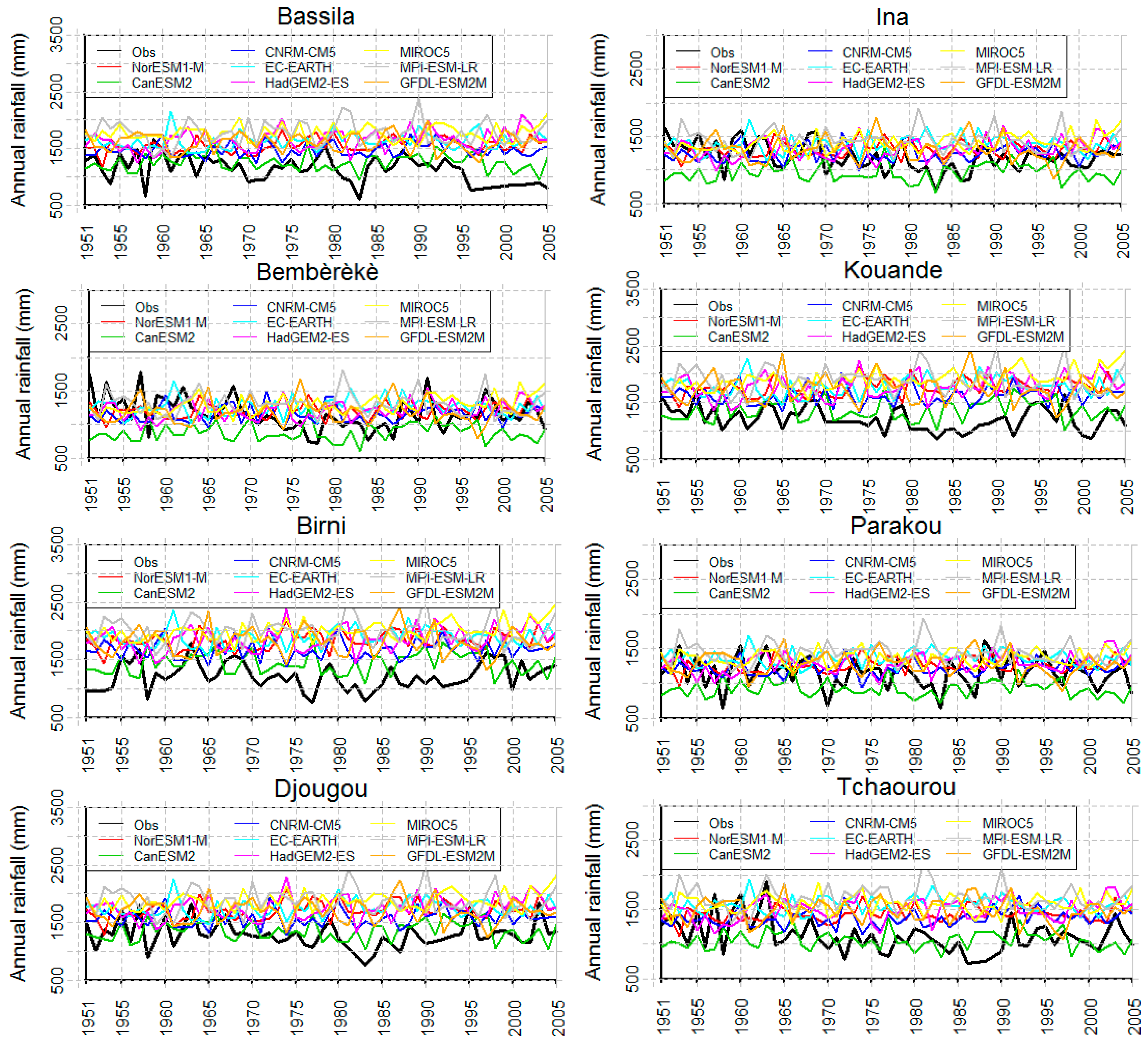
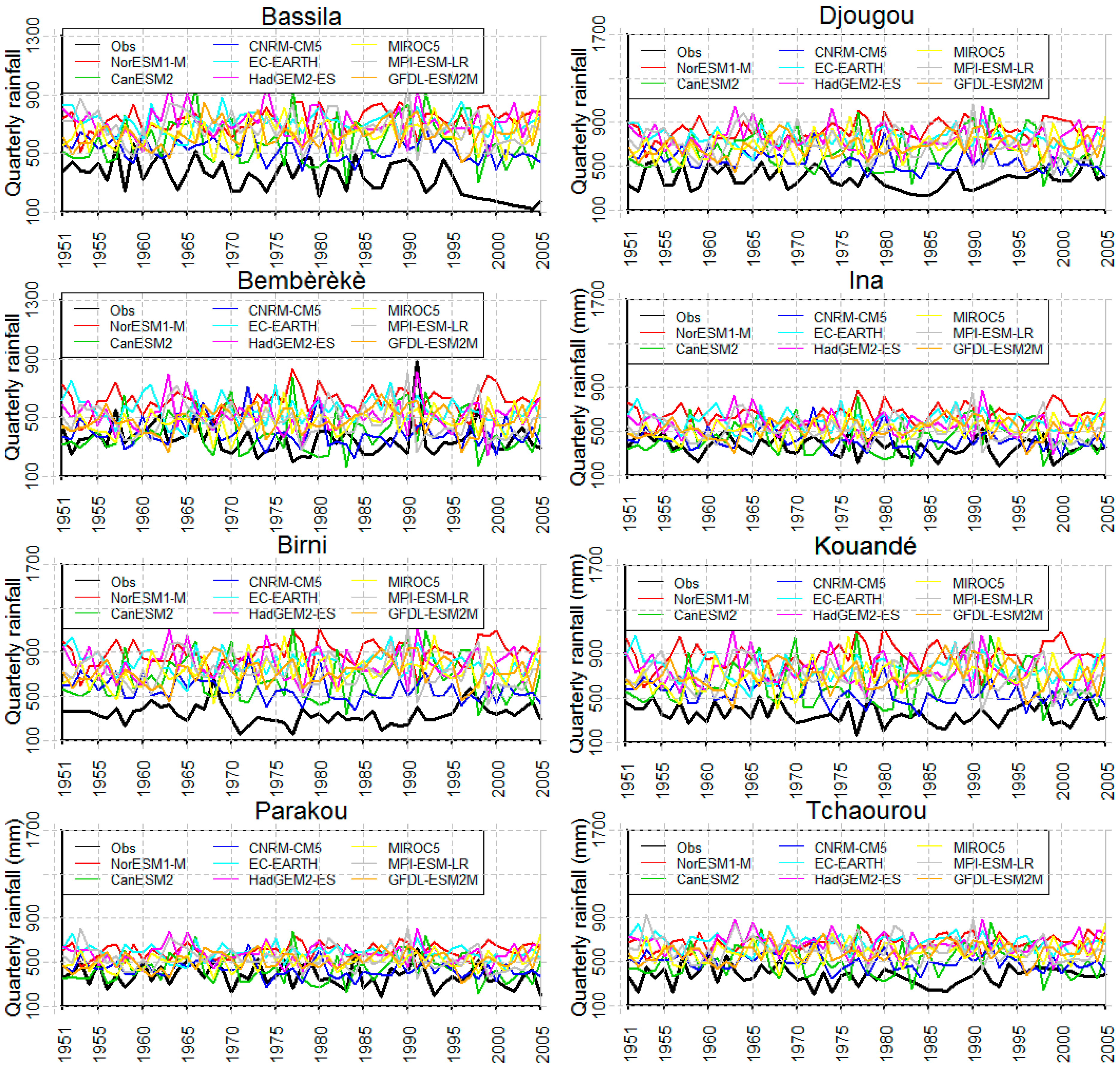
Figure 4 below shows that the data simulated by the eight models generally reproduce the interannual rainfall dynamics quite correctly. However, in terms of amplitude, all models overestimated the annual rainfall accumulation at all stations, except the CanESM2 model which underestimates it in Bembèrèkè, Parakou and Tchaourou. However, as shown in Table 7 below, the average bias for all stations suggests an overestimation of annual rainfall totals for all models, except for the CanESM2 model where there is a very small underestimation (28.84 mm). The MAE and RMSE values are lower for CanESM2. Overall, the CanESM2 model appears to be the best model for simulating annual rainfall totals. It is followed by the CNRM-CM5 model. In all cases, RMSE > MAE, so the errors are not only related to a systematic bias in the average of the simulated totals but also to errors in the interannual variability of the rainfall totals. When the observed data are around 1000 mm, the CanESM2 model reproduces them better. This is the case at the sites of Bassila, Birni, Djougou, Kouandé and Tchaourou. In the case where the observed data are between 1000 and 1500 mm, the other models reproduce the trends of the actual observations. However, the EC-EARTH model is the most accurate, followed by the MIROC5 model.
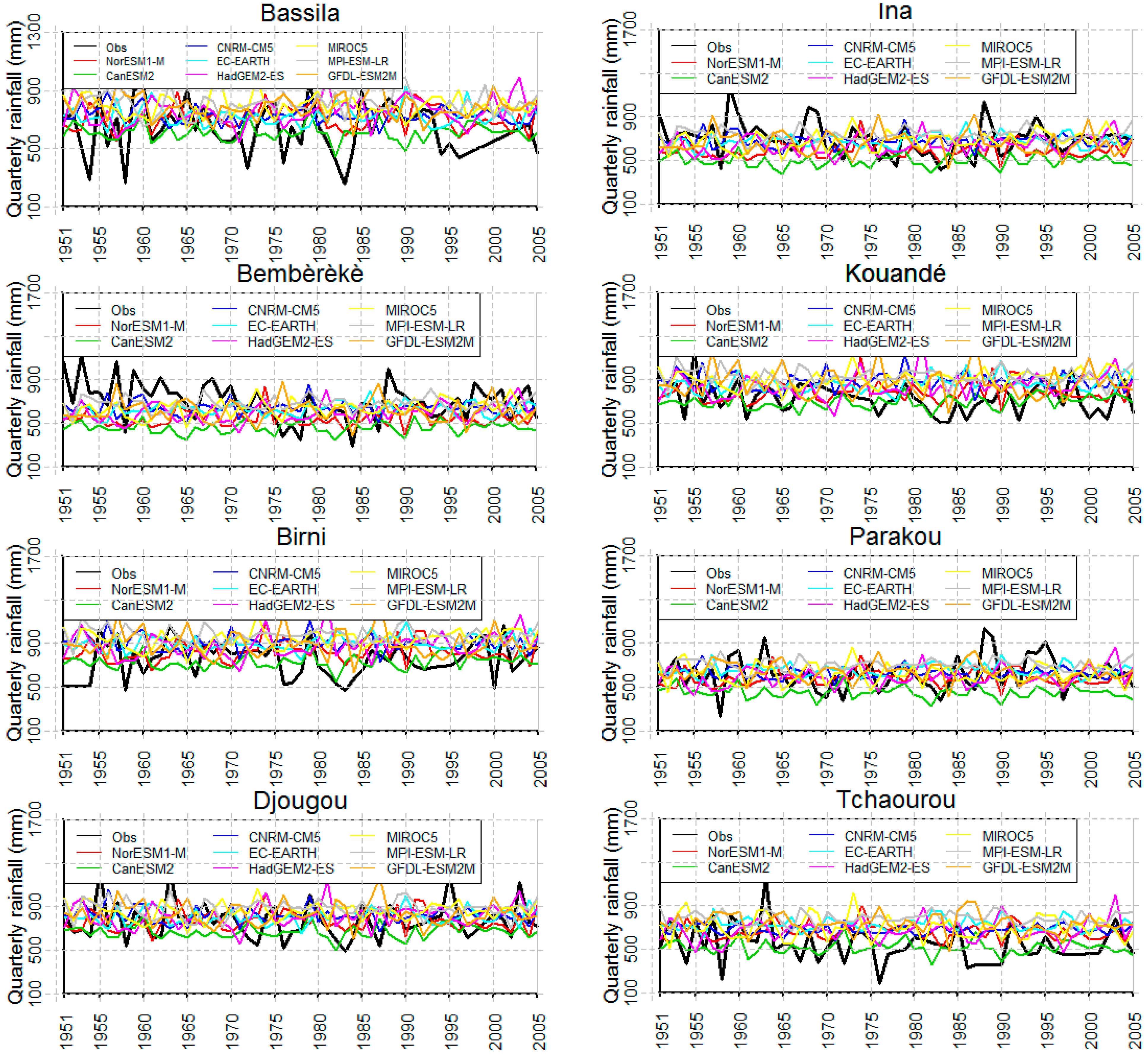
This evolution of annual rainfall accumulation is also observed at the level of seasonal rainfall accumulation (Figure 5). This evolution of seasonal cumulations suggests that the overestimation of annual cumulations by the models is due to the overestimation of seasonal cumulations by the models. Since the average bias, MAE and RMSE are lower for the CanESM2 model (Table 8), this model represents seasonal cumulation well. The CanESM2 model is followed by the CNRM-CM5 model. The very low value (2.619 mm) of the CanESM2 model shows the good accuracy with which it simulates seasonal accumulation.
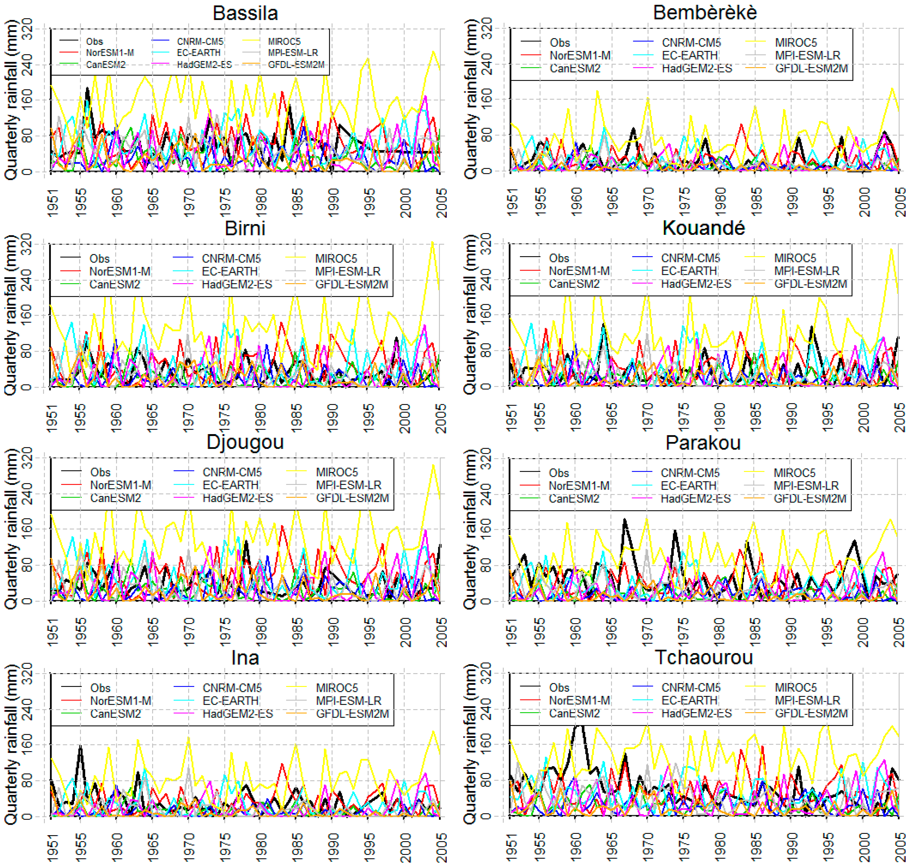
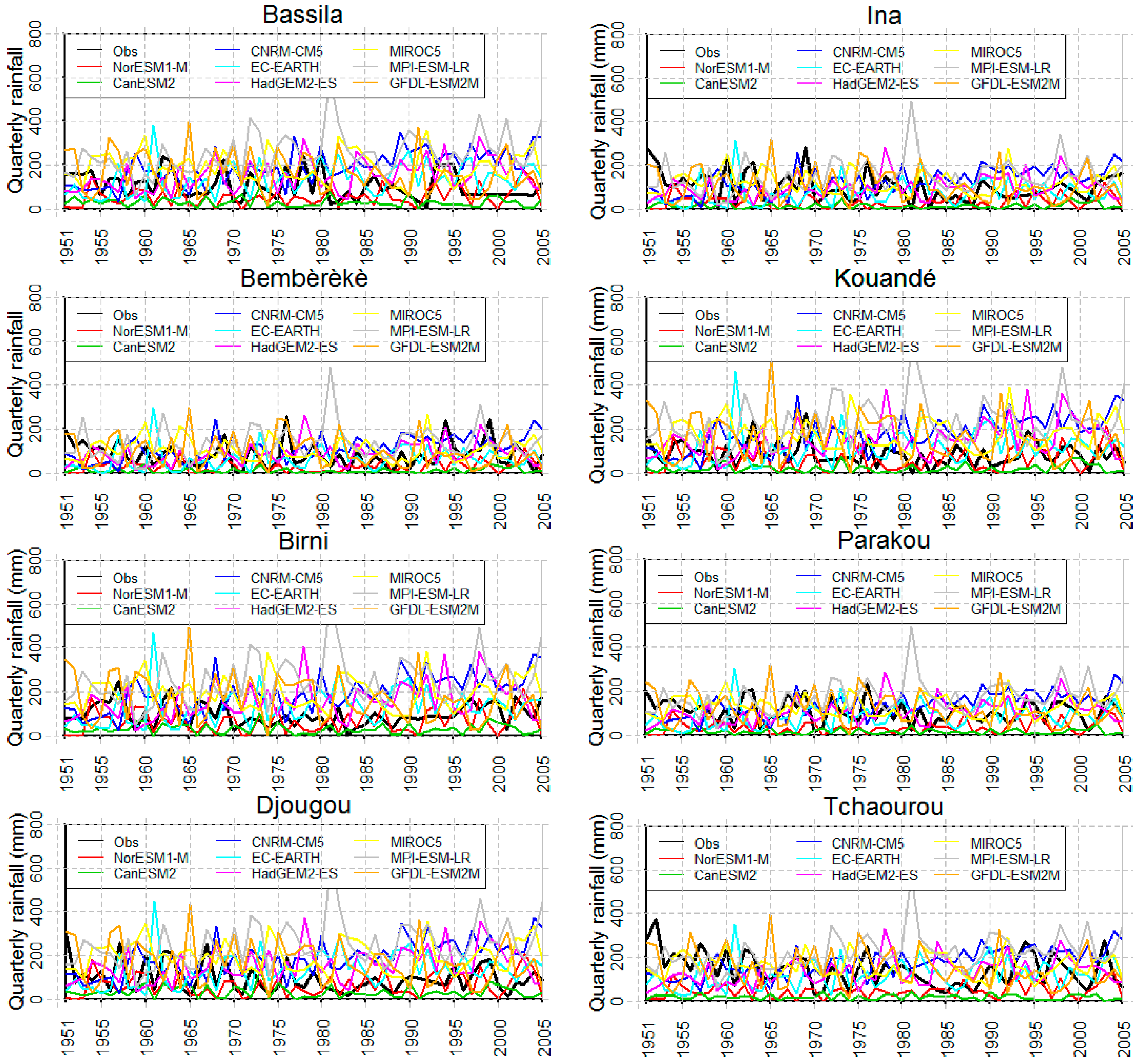
Continuing the analysis with total quarterly precipitation (Figure 6, Figure 7, Figure 8 and Figure 9), the following observations were noted:
In the first quarter (January–February–March: JFM), at all observation sites, all models are representative except the MIROC5 model, which has higher overestimations of quarterly precipitation totals. The average bias is lower for all models except MIROC5, where it is higher (Table 9). The CanESM2, MPI-ESM-LR and GFDL-ESM2M models underestimate the first quarter totals, their bias being negative, while all other models overestimate them. The simulation accuracy is better for EC-EARTH, NorESM1-M, MPI-ESM-LR and HadGEM2-ES models in descending order.
In the second quarter (April–May–June: AMJ), the total of quarterly simulated data from all models follows trends in total of quarterly observed precipitation (Figure 7). However, these cumulations are overestimated by all models, with the average bias being positive everywhere (Table 10). With the lower values of MBE, MAE and RMSE, the CNRM-CM5 model appears more representative. It is followed by the CanESM2 model.
In the third quarter (July–August–September: JAS), the CanESM2 model underestimates precipitation totals (MBE < 0) while all other models overestimate them (Table 11). However, the NorESM1-M and MPI-ESM-LR models have the highest biases. Overall, all models are representative. The quarterly totals of the data simulated by these models perfectly follow the trends of the quarterly totals of observed precipitation (Figure 8). The RMSE values are close for all models.
In the fourth quarter (October–November–December: OND), the CanESM2 model underestimates cumulative precipitation (MBE < 0) while all other models overestimate it (MBE > 0). The MBE and RMSE values are higher for the MPI-ESM-LR model (Table 12). The lowest mean bias is obtained with the EC-EARTH model (MBE = 4.821). This model simulates the fourth quarter totals more accurately. However, the NorESM1-M model has the smallest RMSE value and is therefore the most representative. The oscillations observed in the fourth quarter (Figure 9) suggest that models overestimate the end of season rains, which often occur in October.
In total, the overestimation observed in the second quarter added to that of the fourth quarter at the level of all models explains the overestimations observed at the seasonal level and even at the annual level.
Thus, during the pre-installation period of the West African monsoon (pre-onset) and to some extent during the monsoon recession period, the models overestimate rainfall. In the period when the monsoon is well established (phase onset) the different models better represent the rainfall regime.

3.6. Seasonal Cycles Evolution

At this level of detail, the precipitation 11-day moving average over the period 1956–2005 (Figure 10) follows those of the observations.
Over the first three months, all models except MIROC5 and NorESM1-M represented the daily average precipitation. MIROC5 overestimates the daily average precipitation from mid-February and NorESM1-M overestimates it from mid-March.
From April 1 to the end of June, all models overestimated the daily average precipitation. However, the evolution of the daily average precipitation from the CNRM-CM5 model is much closer to the observations. The average daily precipitation for July and August is better represented by all models. However, from September to December, the CanESM2 and NorESM1-M models underestimate the average daily precipitation at all stations while the CNRM-CM5, MIROC5, MPI-ESM-LR, GFDL-ESM2M and EC-EARTH models represent it well in Bembèrèkè, Ina and Parakou but overestimate it in Bassila, Birni, Djougou, Kouandé and Tchaourou.
In summary, it is noted as indicated above that the start of the rainy season is very poorly simulated by models that have an early start with a high overestimation of rainfall. The end is also poorly simulated with early monsoon withdrawal for CanESM2 and NorESM1-M models and rather late withdrawal for CNRM-CM5, MIROC5, MPI-ESM-LR, GFDL-ESM2M and EC-EARTH models. It should also be noted that, unlike the unimodal observation regime, in a systematic way the models have a bimodal seasonal cycle with a first precipitation peak in May. Thus, the coastal regime is maintained in the models.
The results found in this section confirmed those previously found above at the upper time scales.

3.7. Observed and Simulated Precipitation Indices Comparison

The analysis of Table 13 and Table 14 shows that all models overestimate the CWD and the number of days of heavy rain (R10mm) for all studied stations because the MBE values are positive. On the other hand, the average intensity per rainy day (SDII), CDD, RX1day, R3day, RX5day, number of very heavy rainy days (R20mm), number of extremely heavy rainy days (R25mm), the annual total rainfalls on very rainy days (R95P) and the annual total rain on extremely rainy days (R99P) are underestimated by the models (MBE < 0).
The RMSE values suggest that most indices’ errors are essentially related to a systematic bias in the average of the simulated indices and little or no dependence on errors in interannual variability. However, the slight increase in RMSEs relative to MAEs for the CDD and RX3day indices for most models reveals an additional difficulty in reproducing the interannual variability of number of days of heavy precipitation and the maximum number of consecutive dry days. For the rest, the RMSE and MAE values seem almost identical. The number of rainy days is the most biased index.
In the previous table, the background green color indicates the best estimated indices by each model.

4. Discussion

In this research work, we evaluated the performance of eight general traffic models through the simulations of the RCA4 regional model. Particular attention was paid to precipitation data and some of their characteristics. The performance of a model varies according to the climate parameter taken into account for its evaluation. This is the case, for example, in the studies carried out in Pakistan [8,25], Southeast Asia [2] and West Africa [1]. Similarly, for the same climate parameter, the performance of a model can vary from one statistical criterion to another over the same region. Thus, in the framework of this study, where special attention was paid to precipitation, almost all the models reproduced the interannual variability of precipitation in the upper Ouémé River basin well. This result has already been obtained for West Africa with the regional climate model developed by the Hadley Centre [8]. However, the models overestimated daily rainfall and the number of low rainfall days, especially in the months of April and May. This result therefore explains the simulation of the early start of the rainy season observed with the 11-day moving average calculated over the period 1951–2005. However, the models reproduce well the rainfall in the middle of the rainy season, i.e., from July to September. The late withdrawal of the rainy season observed in the model simulations is explained by the overestimation of the number of rainy days, especially in November. These overestimations of daily rainfall, especially in the months of April, May and November, therefore, explain the models’ overestimation of the cumulative annual and, especially, half-yearly totals. However, the extent of the overestimation varies from one model to another. As for the other rainfall parameters, the models poorly reproduced the rainfall indices (R10mm, R20mm, R25mm, R95p, R99p), the number of consecutive dry days (CDD) and the average intensity per rainy day (SDII). As far as the performance of the models is concerned, it varies from one rainfall parameter to another over the upper Ouémé valley. However, when we look at all the parameters studied, the best performing results of the RCA4 set are MPI-ESM-LR, GFDL-ESM2M, NorESM1-M, and CanESM2. These results are somewhat similar to those obtained for the whole of West Africa [8]. Taking into account the different results obtained in this research when evaluating model performance, the MPI-ESM-LR model can be recommended for future climate change studies on the upper Ouémé River basin. The results of this study can be modified when particular types of assessments are carried out. In addition, model outputs (model ensemble) could be combined because this can increase the skill, reliability and consistency of climate model simulations [26].

5. Conclusions

By comparing the results of the models, we concluded that the CanESM2 model gives lower RMSE values than those produced by the other models, with the correlation coefficient being lower for all models. This model is more effective for simulating daily rainfall, while the MPI-ESM-LR model is more efficient in reproducing the natural variability of the series. For the reproduction of daily rainfall, the CanESM2, CNRM-CM5, EC-EARTH, NorESM1-M, GFDL-ESM2M, MIROC5, MPI-ESM-LR and HadGEM2-ES models can be classified in this order from the most satisfactory to the least satisfactory. However, in the order of the most satisfactory to the least satisfactory, we have for the reproduction of the natural variability of the series the models MPI-ESM-LR, GFDL-ESM2M, NorESM1-M, HadGEM2-ES, MIROC5, EC-EARTH, CNRM-CM5 and CanESM2. Taking into account the precipitation indices, it is rather the following order from most satisfactory to least satisfactory that is obtained: MPI-ESM-LR, GFDL-ESM2M, NorESM1-M, CanESM2, CNRM-CM5, MIROC5, HadGEM2-ES and EC-EARTH.
Thus, it is not easy to say that one model is better than another because all models have advantages and limitations. The best way is to work with several methods and compare the results. Moreover, scenario results must be analyzed and interpreted carefully. In our opinion, general circulation models still require a great deal of research in order to produce more satisfactory results in the upper Ouémé River basin with respect to the simulation of daily precipitation. However, by combining the results obtained for the various parameters considered in this study, it can be concluded that the MPI-ESM-LR model is more satisfactory for rain simulation in the upper Ouémé River basin, followed in decreasing order of satisfaction by the GFDL-ESM2M, NorESM1-M, CanESM2, CNRM-CM5, MIROC5, HadGEM2-ES and EC-EARTH models.

Author Contributions

A.A., J.-F.D. and A.E.L. designed the study, developed the methodology and wrote the manuscript, A.A. performed the field work, collected the data and conducted the computer analysis, while J.-F.D. and A.E.L. supervised the work. All authors have read and agreed to the published version of the manuscript.

Funding

This research received no external funding.

Acknowledgments

This research described in this article was simultaneously developed at the Laboratory of Applied Hydrology and the International Chair in Physics, Mathematics and Applications of the University of Abomey-Calavi and at Aquapole of University of Liege.

Conflicts of Interest

The authors declare no conflict of interest.

References

  1. Gnitou, G.T.; Ma, T.; Tan, G.; Ayugi, B.; Nooni, I.K. Evaluation of the Rossby Centre Regional Climate Model Rainfall Simulations over West Africa Using Large-Scale Spatial and Temporal Statistical Metrics. Atmosphere 2019, 10, 802. [Google Scholar] [CrossRef] [Green Version]
  2. Kamworapan, S. Evaluation of CMIP5 Global Climate Models for Simulating Climatological Temperature and Precipitation for Southeast Asia. Adv. Meteorol. 2019, 2019, 1067365. [Google Scholar] [CrossRef]
  3. Tolika, K.; Maheras, P.; Vafiadis, M.; Anagnostopoulou, C. Comparaison de deux scenarios (statistique et dynamique) concernant les precipitations hivernales. Climatologie 2007, 4, 73–90. [Google Scholar] [CrossRef]
  4. Dutrieux, P. Évaluation de simulations du modèle régional canadien du climat (MRCC5) au-dessus de l’atlantique nord. In Mémoire de la Maîtrise en Sciences de L’atmosphère; Université du Québec à Montréal: Montréal, QC, Canada, 2016; p. 125. [Google Scholar]
  5. Bader, D.C.; Covey, C.; Gutowski, W.J., Jr.; Held, I.M.; Kunkel, K.E.; Miller, R.L.; Tokrnakian, R.T.; Zhang, M.H. A Report by the U.S. Climate Change Science Program and the Subcommittee on Global Change Research. In Climate Models: An Assessment of Strengths and Limitations; Department of Energy, Office of Biological and Environmental Research: Washington, DC, USA, 2008; p. 124. [Google Scholar]
  6. Laprise, R.; de Elía, R.; Caya, D.; Biner, S.; Lucas-Picher, P.; Diaconescu, E.; Leduc, M.; Alexandru, A.; Separovic, L. Challenging some tenets of Regional Climate Modelling. Meteorol. Atmos. Phys. 2008, 100, 3–22. [Google Scholar] [CrossRef]
  7. Leung, L.R.; Mearns, L.O.; Giorgi, F.; Wilby, R.L. Regional climate research. Bull. Am. Meteorol. Soc. 2003, 84, 89–95. [Google Scholar]
  8. Khan, N.; Shahid, S.; Ahmed, K.; Ismail, T.; Nawaz, N.; Son, M. Model in Simulating Daily Precipitation and. Water 2018, 10, 1793. [Google Scholar] [CrossRef] [Green Version]
  9. Le Treut, H. Évolution Climatique: Les Modèles et Leurs Limites. Available online: http://www.cnrs.fr/publications/imagesdelaphysique/couv-PDF/IdP2005/05Letreut.pdf (accessed on 12 July 2016).
  10. Giannini, A.; Biasutti, M.; Held, I.M.; Sobel, A.H. A global perspective on African climate. Clim. Chang. 2008, 90, 359–383. [Google Scholar] [CrossRef]
  11. Biasutti, M.; Giannini, A. Robust Sahel drying in response to late 20th century forcings. Geophys. Res. Lett. 2006, 33, 10–13. [Google Scholar] [CrossRef] [Green Version]
  12. Hoerling, M.P.; Hurrell, J.W.; Xu, T. Tropical origins for recent North Atlantic climate change. Science 2001, 292, 90–92. [Google Scholar] [CrossRef] [PubMed] [Green Version]
  13. GIEC. Bilan 2007 des Changements Climatiques. Contribution des Groupes de Travail I, II et III au Quatrième Rapport D’évaluation du Groupe D’experts Intergouvernemental sur L’évolution du Climat [Équipe de Rédaction Principale, Pachauri, R.K. et Reisinger, A. (Publié Sous la Direction de~)]. GIEC: Genève, Suisse, 2007. Available online: https://www.ipcc.ch/site/assets/uploads/2018/02/ar4_syr_fr.pdf (accessed on 12 July 2018).
  14. Kamga Foamouhoue, A.; Buscarlet, E. Simulation du climat de l’Afrique de l’Ouest à l’aide d’un modèle climatique régional: Validation sur la période 1961–1990. La Météorologie 2006, 8, 28. [Google Scholar] [CrossRef] [Green Version]
  15. COI. Synthèse des Travaux du Projet Acclimate de la Commission de L’océan Indien Alexandre Magnan, Virginie, Duvat. 2012. Available online: http://www.commissionoceanindien.org/archives/society.ioconline.org/fileadmin/Acclimate/SYNTHESE Accli681 mate_01.pdf1 (accessed on 5 January 2015).
  16. Giorgi, F.; Jones, C.; Asrar, G.R. Addressing Climate Information Needs at the Regional Level: The CORDEX Framework. Bulletin 2009, 58, 3. [Google Scholar]
  17. Mahé, G.I.L.; Triboulet, J.P. Analysis of a Sahelian annual rainfall index from 1896 to 2000; the drought continues. Hydrol. Sci. J. 2002, 47, 563–572. [Google Scholar]
  18. Olivry, J.-C. De l’évolution de la puissance des crues des grands cours d’eau intertropicaux d’Afrique depuis deux décennies. Rev. Geogr. Alp. 1994, 12, 101–108. [Google Scholar]
  19. Gachon, L.G.; Bokoye, A.I.; Parishkura, D.; Cotnoir, A.; Tramblay, Y.; Vigeant, G. Groupe de travail II Variabilité, extrêmes et changements climatiques au Sahel: De l’observation à la modélisation. In dans Rapport des Contributions Canadiennes au Projet ACDI—CILSS (#A030978-002); Appui Aux Capacités D’adaptation Aux Changements Climatiques; Environnement Canada: Montréal, QC, Canada, 2007. [Google Scholar]
  20. Willmott, C.J.; Matsuura, K. Advantages of the mean absolute error (MAE) over the root mean square error (RMSE) in assessing average model performance. Clim. Res. 2005, 30, 79–82. [Google Scholar] [CrossRef]
  21. Willmott, C.J.; Matsuura, K.; Robeson, S.M. Ambiguities inherent in sums-of-squares-based error statistics. Atmos. Environ. 2009, 43, 749–752. [Google Scholar] [CrossRef]
  22. Chai, T.; Draxler, R.R. Root mean square error (RMSE) or mean absolute error (MAE)? -Arguments against avoiding RMSE in the literature. Geosci. Model. Dev. 2014, 7, 1247–1250. [Google Scholar] [CrossRef] [Green Version]
  23. Ansari, A.R.; Bradley, R.A. Rank-sum tests for dispersions. Ann. Math. Stat. 1960, 31, 1174–1189. [Google Scholar] [CrossRef]
  24. Kostopoulou, E.; Giannakopoulos, C.; Anagnostopulou, C.H.R.; Tolika, K.; Maheras, P.; Vafiadis, M. Simulating Maximum and Minimum temperatures over Greece: A comparison of three modeling techniques. Theor. Appl. Climatol. 2006, 90, 65–82. [Google Scholar] [CrossRef]
  25. Ahmed, K.; Sachindra, D.A.; Shahid, S.; Demirel, M.C.; Chung, E. Selection of multi-model ensemble of general circulation models for the simulation of precipitation and maximum and minimum temperature based on spatial assessment metrics. Hydrol. Earth Syst. Sci. 2019, 23, 4803–4824. [Google Scholar] [CrossRef] [Green Version]
  26. Tebaldi, C.; Knutti, R. The use of the multi-model ensemble in probabilistic climate projections. Philos. Trans. R. Soc. A Math. Phys. Eng. Sci. 2007, 365, 2053–2075. [Google Scholar] [CrossRef] [PubMed]
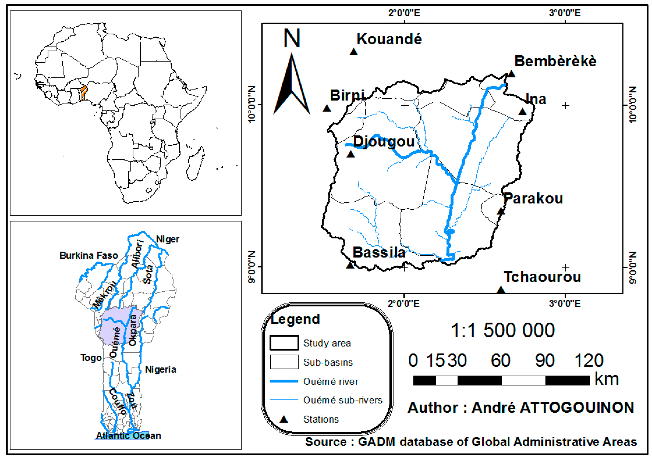
Figure 1. Location of the study area.
Hydrology 07 00011 g001
Figure 2. Boxplot of observed and simulated daily rainfalls over the period 1951–2005.
Hydrology 07 00011 g002aHydrology 07 00011 g002b
Figure 3. Density of observed and simulated precipitations.
Hydrology 07 00011 g003
Figure 4. Compared evolution of the total annual observed and simulated rainfall.
Hydrology 07 00011 g004
Figure 5. Compared evolution of the total seasonal of observed and simulated rainfall.
Hydrology 07 00011 g005
Figure 6. First quarter total rainfall evolution.
Hydrology 07 00011 g006
Figure 7. Second quarter total rainfall evolution.
Hydrology 07 00011 g007
Figure 8. Third quarter total rainfall evolution.
Hydrology 07 00011 g008
Figure 9. Fourth quarter total rainfall evolution.
Hydrology 07 00011 g009
Figure 10. Comparison of observed and simulated data seasonal cycles.
Hydrology 07 00011 g010aHydrology 07 00011 g010b
Table 1. List of selected stations in the upper Ouémé River basin.
StationsBenin Meteo Agency CodeLong. (Degrees)Lat. (Degrees)Elevation (m)
BassilaD0371.6679.017384
BembèrèkèD0242.66210.223491
BirniD0261.5179.983430
DjougouD0301.6629.692439
InaD0272.7279.969358
KouandéD0191.68310.333442
ParakouD0342.6129.357392
TchaourouD0382.600325325
Table 2. Presentation of global climate models selected for the study.
Research CentersAcronym(s) for CentersModel NameResolution (Long. × Lat.; Degrees)
Canadian Centre for Climate Modelling and Analysis CanadaCCCmaCanESM22.81 × 2.79
Centre National de Recherches Météorologiques, Centre Européen de Recherche et de Formation Avancée en Calcul Scientifique FranceCNRM-CERFACSCNRM-CM51.41 × 1.4
EC-EARTH consortium published at Irish Centre for High-End Computing Netherlands/IrelandICHECEC-EARTH1.13 ×1.12
Atmosphere and Ocean Research Institute (The University of Tokyo), National Institute for Environmental Studies, and Japan Agency for Marine-Earth Science and Technology JapanMIROCMIROC51.41 × 1.39
Met Office Hadley Centre EnglandMOHCHadGEM2-ES1.875 × 1.25
Max Planck Institute for Meteorology GermanyMPI-MMPI-ESM-LR1.875 × 1.85
Bjerknes Centre for Climate Research, Norwegian Meteorological Institute NorwayNCC, NMINorESM1-M1.875 × 1.85
Geophysical Fluid Dynamics Laboratory USANOAA-GFDLGFDL-ESM2M2.5 × 2.0
Table 3. Definition of indices.
IndicesNameIndices CalculationDefinitionUnit
Frequency Indices (adapted from WMO 2009)
R10mmNumber of heavy rainfall daysRRij 10 mmAnnual count of days when days rainfall 10 mmDays
R20mmNumber of very heavy rainfall daysRRij 20 mmAnnual count of days when days rainfall 20 mmDays
R25mmNumber of extremely heavy rainfall days RR ij 25   mm Annual count of days when days rainfall 25 mmDays
CDDConsecutive dry days RR ij < 1   mm Maximum number of consecutive days with RR < 1 mmDays
CWDConsecutive wet days RR ij 1   mm Maximum number of consecutive days with RR 1 mmDays
Intensity Indices (adapted from WMO 2009)
SDIISimple daily intensity index SDII j = w = 1 W RR wj W Annual mean rainfall when PRCP > 1 mmmm/day
RX1dayMaximum daily rainfall Rx 1 day j = max ( RR ij ) Maximum 1-day Rainfallmm
RX3dayMaximum 3-day rainfallRx3dayj = max(RRij)Maximum 3-day rainfallmm
RX5dayMaximum 5-day rainfallRx5dayj = max(RRij)Maximum 5-day rainfallmm
R95pVery wet day R 95 P j = w = 1 W R wj Annual total rainfall when RR > 95 percentilemm
R99pExtremely wet day R 99 P J = w = 1 W R wj Annual total rainfall when RR > 99 percentilemm
Table 4. Correlation coefficients between observed and simulated precipitation for each station by general circulation model.
CanESM2CNRM-CM5EC-EARTHHadGEM2-ESMIROC5MPI-ESM-LRNorESM1-MGFDL-ESM2M
Bassila0.1840.1910.176−0.0410.1640.1610.1690.181
Bembèrèkè0.1690.1790.180−0.0420.1680.1690.1730.183
Birni0.1980.2230.207−0.0660.1900.1960.1960.200
Djougou0.2060.2130.189−0.0500.1690.1950.1980.203
Ina0.1780.2080.195−0.0490.1910.1940.1690.190
Kouandé0.1920.2110.203−0.0580.1950.2040.1790.199
Parakou0.1550.1820.165−0.0420.1460.1640.1590.159
Tchaourou0.1540.1750.171−0.0440.1400.1740.1490.172
Table 5. Deviations of standard deviations of observed and simulated precipitations by models over the period 1951–2005.
CanESM2CNRM-CM5EC-EARTHHadGEM2-ESMIROC5MPI-ESM-LRNorESM1-MGFDL-ESM2M
Bassila−4.038−3.467−3.299−3.124−3.014−2.47−3.168−2,825
Bembèrèkè−5.562−4.511−4.711−4.583−4.581−4.07−4.572−4,615
Birni−3.853−3.247−2.991−2.864−2.959−2.32−2.833−2.808
Djougou−4.508−3.996−3.805−3.589−3.685−3.01−3.633−3.513
Ina−4.966−4.041−4.087−4.022−4.033−3.47−3.981−3.998
Kouandé−3.833−3.032−2.983−2.819−2.892−2.29−2.729−2.832
Parakou−5.574−4.839−4.645−4.631−4.630−3.97−4.579−4.541
Tchaourou−4.369−3.731−3.307−3.245−3.184−2.69−3.267−3.052
mean−4.588−3.858−3.729−3.609−3.622−3.04−3.595−3.523
Table 6. Mean values of MBE, MAE and RMSE between observed and simulated precipitation by models for all stations.
CanESM2CNRM-CM5EC-EARTHHadGEM2-ESMIROC5MPI-ESM-LRNorESM1-MGFDL-ESM2M
MBE0.3490.9481.3891.3951.7731.7741.1731.326
MAE4.6454.9665.3096.4415.6305.5795.2105.228
RMSE9.2499.4679.66110.8349.90510.1719.7209.834
Table 7. Results of statistical criteria for annual rainfall accumulation.
MBEMAERMSE
CanESM2−28.84276.02340.22
CNRM-CM5233.82313.81370.75
EC-EARTH393.69438.35499.13
HadGEM2-ES359.82423.53483.06
MIROC5465.35499.47552.99
MPI-ESM-LR484.26518.63588.60
NorESM1-M324.20391.89451.12
GFDL-ESM2M330.62400.24476.57
Table 8. Results of statistical criteria for seasonal cumulation.
MBEMAERMSE
CanESM22.62266.37330.19
CNRM-CM5257.92320.84376.33
EC-EARTH392.78431.29489.14
HadGEM2-ES371.49426.76483.15
MIROC5375.24422.41478.15
MPI-ESM-LR484.71512.75578.13
NorESM1-M325.92381.52441.24
GFDL-ESM2M357.47411.49486.63
Table 9. Results of statistical criteria for first quarter total precipitation.
MBEMAERMSE
CanESM2−22.3534.5744.99
CNRM-CM523.1333.2044.74
EC-EARTH1.4438.0949.80
HadGEM2-ES14.7837.5349.82
MIROC573.7880.6196.35
MPI-ESM-LR−11.7936.2246.40
NorESM1-M5.5938.7849.16
GFDL-ESM2M−25.0234.7146.49
Table 10. Results of statistical criteria for second quarter total precipitation.
MBEMAERMSE
CanESM2175.86221.80274.20
CNRM-CM5130.02156.93185.79
EC-EARTH317.09319.75344.76
HadGEM2-ES302.55308.02340.29
MIROC5246.64260.30293.04
MPI-ESM-LR257.90268.62305.08
NorESM1-M369.46373.58401.31
GFDL-ESM2M242.52252.48286.50
Table 11. Results of statistical criteria for third quarter total precipitation.
MBEMAERMSE
CanESM2−100.75172.99209.05
CNRM-CM566.37159.27196.17
EC-EARTH70.35168.39206.76
HadGEM2-ES44.49170.21210.89
MIROC588.36178.54218.08
MPI-ESM-LR131.96190.90229.99
NorESM1-M369.46373.58201.33
GFDL-ESM2M73.15179.87228.97
Table 12. Results of statistical criteria for fourth quarter total precipitation.
MBEMAERMSE
CanESM2−81.6185.41104.73
CNRM-CM560.57102.69120.39
EC-EARTH4.8282.89105.89
HadGEM2-ES27.5679.68100.46
MIROC556.0387.87109.27
MPI-ESM-LR106.17125.90157.62
NorESM1-M54.3775.7095.54
GFDL-ESM2M39.9894.17119.69
Table 13. Average of the statistical criteria of the indices for all the stations studied.
CanESM2 ModelCNRM-CM5 ModelEC-EARTH Model
MBEMAERMSEMBEMAERMSEMBEMAERMSE
CWD32.9932.9933.8243.1843.1843.8447.4147.4147.99
SDII−7.827.828.38−7.267.277.82−6.926.937.52
CDD−3.276.328.47−2.296.338.07−6.597.879.68
RX1day−50.8151.6456.79−39.2045.8752.73−39.3640.0549.81
R3day−44.7546.2553.86−32.4843.9953.00−31.0438.6447.26
RX5day−43.2046.2356.27−32.5843.4853.99−28.2040.3751.19
R10mm1.3714.2617.2812.0015.5517.8119.5421.5424.22
R20mm−16.7616.8317.89−15.5215.5316.63−14.6114.6515.97
R25mm−13.3313.3314.17−12.6412.6413.55−12.2312.2213.20
R95P−100.79103.84121.96−57.8280.1099.00−43.7071.4988.88
R99P−32.8635.2443.26−16.8635.1345.62−19.5231.3540.53
HadGEM2-ES ModelMIROC5 ModelMPI-ESM-LR Model
MBEMAERMSEMBEMAERMSEMBEMAERMSE
CWD45.7945.7946.4248.0848.0848.6247.5447.5448.19
SDII−6.596.917.52−7.117.117.69−6.44−6.477.10
CDD−6.597.659.47−7.577.879.92−6.017.519.33
RX1day−39.7644.1950.81−34.9339.7346.33−31.4339.7547.09
R3day−31.0938.6447.22−25.8936.0743.84−21.6637.9948.15
RX5day−28.9238.1948.72−24.4937.3347.29−19.9137.6249.22
R10mm20.0022.2724.9917.1220.3422.7726.2727.3730.34
R20mm−14.0914.2115.45−14.4814.5415.80−11.7712.1113.55
R25mm−12.2612.2613.23−12.2212.2213.11−11.1611.1812.23
R95P−44.4870.0588.43−36.0966.2184.60−13.2868.1888.06
R99P−16.5633.0442.16−10.6630.7539.49−2.7032.9045.21
Table 14. Average of the statistical criteria of the indices for all the stations studied (continued).
NorESM1-M ModelGFDL-ESM2M Model
MBEMAERMSEMBEMAERMSE
CWD43.3243.3243.9844.7344.7345.57
SDII−6.876.877.47−6.866.877.48
CDD−5.117.599.57−4.326.978.95
RX1day−36.2740.9248.04−34.9538.9146.24
R3day−28.0237.1345.19−25.8935.0844.26
RX5day−23.7637.4546.96−22.1037.9947.75
R10mm16.3819.3021.8017.8920.9224.43
R20mm−13.9514.0315.33−13.3913.8015.05
R25mm−12.0212.0212.96−11.6211.6512.67
R95P−43.0569.3987.67−34.8468.5685.09
R99P−11.6930.7440.38−9.2729.9538.88