The Storage and Water Quality Characteristics of Rungiri Quarry Reservoir in Kiambu, Kenya, as a Potential Source of Urban Water

Abstract

Urbanization has caused limitations on water resources, while climate change has reduced amounts of surface water in some parts of the world. Kikuyu, a suburban area in Kiambu county, Kenya, is facing this challenge. The major challenge in the study is scarcity of potable water, resulting in inadequate water supply to Kikuyu residents. Currently, only 63.6% of the population is being supplied with water by Kikuyu Water Company, the company mandated to supply water to the area. Water demand was 2972 m³/day in 2015 and was projected to be 3834 m³/day by 2025. This has put pressure on the already exploited clean water resources, making it necessary to seek additional sources of domestic water. Storage capacity and water quality of surface water bodies, especially small reservoirs whose water can be used to ease the demand, need to be assessed for supplemental water supply. This study aimed at assessing the suitability of the abandoned quarry reservoir as a source of potable urban water by determining its storage capacity characteristics and water quality status. Volume characteristics were determined using bathymetry survey in January 2019. Water samples were collected in January and August 2019 and analyzed for chemical, physical, and bacteriological quality, as per the American Public Health Association (APHA) standard methods for water and wastewater. Parameters were evaluated based on World Health Organization (WHO) and Kenya Bureau of Standards (KEBS) guidelines for drinking water, and rated based on the drinking water quality index (WQI). The reservoir’s maximum storage capacity was found to be 128,385 m³, the surface area was 17,699 m², and the maximum depth was 15.11 m. Nineteen of the twenty-five investigated parameters were within the acceptable standards. However, the concentrations of manganese (Mn), cadmium (Cd), iron (Fe), turbidity, total coliforms, and Escherichia coli (E. coli) were above the acceptable limits. Manganese and iron levels increased with depth. The overall WQI of the reservoir was 82.51 and 85.85 in January and August, respectively. Therefore, based on WQI rating, the water scored a good quality rating and could be used for domestic supply upon treatment. The original achievement of this study is establishment of the volume of the water in the quarry as an additional source of water to the nearby community, along with water quality status.

1. Introduction

Urbanization has led to constraint of water resources, while climate change has reduced amounts of surface water in some parts of the world [1]. Normally, underground mine galleries and open-pit mines are flooded by natural groundwater, surface water inflow, and water pumped from dewatering systems, and can therefore be used as strategic reservoirs for water storage. Depending on its quality and intended purpose, water is treated using appropriate technology to meet different needs [1]. Water in quarry reservoirs can be used for irrigation, domestic supply, industrial supply, and aquifer recharge, amongst other uses [2]. The Hallett quarry gravel pit lake system in Ames City, Iowa, United States, is one of the quarry pits that was assessed for water storage and domestic supply to the city [3]. The quarry pit system water was analyzed together with the effect of storm water. The water quality was found to be of similar quality when compared to other water bodies in Iowa. Storm water elevated concentration of parameters such as fecal coliforms in the quarry pit system [3]. Bellwood quarry in Atlanta, Georgia, is also used for raw water storage to supplement existing water supply [4]. Kikuyu sub-county in Kiambu county, Kenya, has few surface water resources and mostly relies on groundwater resources [5]. Kikuyu Water Company, which is mandated to supply water to the sub-county, is not able to meet the current water demand. According to a report on the performance of Kenya’s water service sector, only 202,582 persons out of a total population of 318,557 persons within the company’s mandated area are being supplied with water by the company [6]. The water demand in Kikuyu in 2015 was 2972 m³/day and was projected to be 3834 m³/day in 2025. It is, therefore, important to exploit any possible sources of water in the area to ease the current and future water demand. Small reservoirs have been neglected in hydrological research. They receive less attention and lack management strategies, while large reservoirs are well managed and monitored [7]. Rungiri quarry reservoir, whose storage capacity and water quality is unknown, could be a potential source of water for the neighbouring community. The reservoir is 2.5 km from Kikuyu town, which Kikuyu Water Company solely supplies water to. The reservoir was formed in 1992 during quarrying of trachyte for road construction as a result of puncturing a ground water aquifer, and has been used for irrigation ever since, with the excess water being unutilized [8]. The other natural water body within the area is Kikuyu springs, which is currently under development to supply water to Kikuyu town and its environs. Rungiri quarry reservoir is a potential source. The water source is purely ground water. The county government of Kiambu is interested in the reservoir for domestic water supply, so the results of this study will be timely.

Knowledge of available water in reservoirs guides stakeholders and managers in determining sustainable exploitation plan of the reservoirs [9]. Water body morphometry parameters provide information to assess residence time, life expectancy, water balance, sustainable water abstraction, and derivation of stage curves [10]. Some of the methods used to assess storage capacities of reservoirs are bathymetry surveys. Bathymetry refers to depths and shapes of underwater terrain [11]. There are different methods used to generate bathymetric information, such as spatial interpolation methods based on collected depth samples, topographic-data-based methods, and remote-sensing-based methods. Spatial interpolation methods are the most frequently used to obtain bathymetric information [12]. Topographic-data-based methods allow mapping of the bathymetry of reservoirs easily compared to the other methods; however, the topographic data must be collected before filling the reservoir, and these kinds of data are not always available. Remote sensing-based methods have advantages in terms of the coverage of large areas and data collection in areas with limited access. Remote-sensing-based methods are limited by the water transparency, the depth of the reservoir, and meteorological conditions [12]. However, remote sensing by light detection and ranging (LIDAR) and bathymetry survey by use of an acoustic profiling system (APS) offer comparable accuracy [13]. To ensure proper coverage of a water body in a bathymetry survey, APS is used. 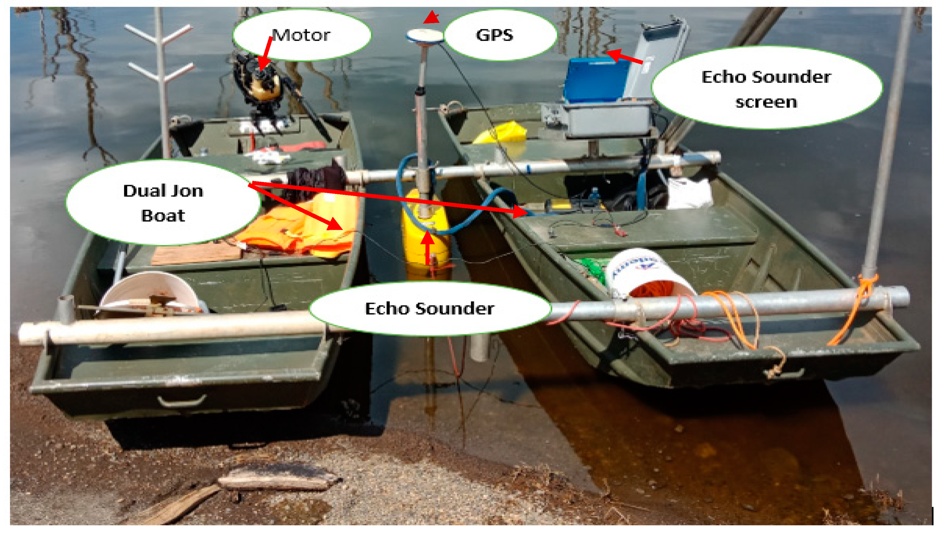LIDAR may offer comparable accuracy to bathymetry survey but is expensive, equipment intensive, and time consuming [13,14] Bathymetric survey by use of APS is a fast and low cost methodology that gives detailed information on water depths, surface areas, and reservoir depth-volume relationships by use of sound in measurement of water depths. This technique has been used globally to avail data for volume computation of water in reservoirs, generation of depth contour maps, and underwater morphology. By using APS, water depth information in the form of x, y, z coordinates is obtained by conducting a sequence of cross-sectional surveys in the water body along multiple transects [15].

Similar surveys have been done in the Peechi reservoir, Ruiru reservoir, and lake Naivasha [9,11,16] Bathymetric maps, storage capacities, and morphometric characteristics of Lake Hayq in Ethiopia were generated to provide scientific information for use in reservoir management [10]. Bathymetry survey data was used to estimate storage capacities of small reservoirs in the upper-eastern region of Ghana [17,18,19,20]. Hydrographic surveys for sea beds and lakes provide key information on morphology of waterbodies However, use of APS in bathymetry surveys makes it challenging to obtain depth measurements at depths of less than 50 cm. Regions of lower depth are not surveyed but are generated with interpolation techniques or direct measurement of water depth [9]. Techniques used for interpolation of bathymetry survey data include triangulated irregular network (TIN) model, nearest-neighbor interpolation, kriging interpolation method, inverse distance interpolation, and polynomial interpolation. Kriging method is the most suitable for interpolating single-beam data [18], and according to [10], the kriging interpolation method produces visually appealing maps by reducing interpolation errors. A study done to compare different spatial interpolation methods for historical hydrographic data of the lowermost Mississippi river by [15] concluded that ordinary kriging performed best in mapping the bathymetry of the river.

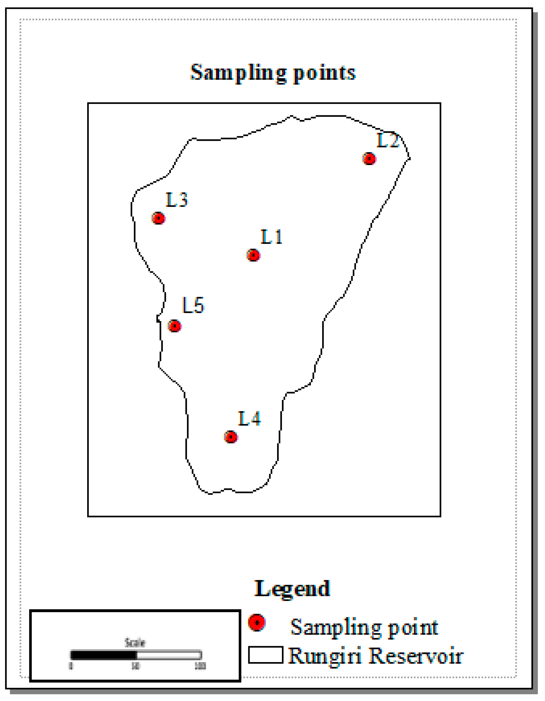
The methodology was developed specifically for reservoirs. For this particular case, it was applied to a quarry and utilized in determination of precise depth and geographical coordinates of water sample collection points in both January and August, unlike in the previous studies.

Providing safe drinking water to the population is one of Kenya’s Vision 2030 goals. Safe drinking water is not only important for health, but has a considerable role in development at national, regional, and local levels. Investment in water supply and sanitation yield a net economic benefit [21].

Water quality directly affects water purification and treatment costs [22], hence making it an important part of water supply functionality. The main reasons for testing water quality is the need to assess various parameter statuses against existing standards and to verify whether the observed water quality is suitable for prospective uses. The level of contamination necessary to render a water body impaired is highly dependent on the type of water body, location, and the types of beneficial uses it supports [23]. Surface water is affected by weathering of rocks, erosion, decay of organic matter, industrial and domestic water waste, agricultural runoff containing fertilizers, pesticides, and herbicides, and thermal wastes [24]. For instance, heavy metal contamination in non-industrial or agricultural catchment setups contain metals in their geochemical background level or can be slightly contaminated [25]. For health purposes, drinking water parameters should be within the standards set by Kenya Bureau of Standards (KEBS) and World Health Organization (WHO) guidelines to ensure safety.

Parameter quality when compared with guideline values indicates the acceptability of that specific parameter. The Water Quality Index (WQI), on the other hand, describes the influence of water quality parameters on the overall quality of water [26]. Unlike the traditional methods, where an individual water quality parameter is compared with its standard limit with no depiction of water quality status [27], the WQI reduces the large amounts of information to a single number, which reflects the composite influence of various quality parameters on the overall quality of water [28]. It is utilized when surveying the general water quality by utilizing a finite scale to differentiate between polluted water and very clean water [29]. WQI gives important data on the general water quality status, which can help in choosing a suitable water treatment technique [28]. Models are also efficient tools, especially in forecasting water quality parameters in water bodies. Examples of these models are ensemble models and machine learning models, which are either data-driven models or physically based models [30,31]. However, modelling and forecasting of water quality is a complex procedure because of the nonlinear relationship of the variables [31].

The WQI was first introduced by Horton in the early 1970s as a means of calculating a single value from many test results to represent the level of water quality in a given water body. This was done in order to report large amounts of data in an understandable manner that is useful to the public and policy makers [26]. According to Abbasi (2012), water quality indices can be of two groups: “water pollution indices”, in which the index numbers increase with the degree of pollution (increasing scale indices); and “water quality indices”, in which the index numbers decrease with the degree of pollution (decreasing scale indices) [32]. The common water quality indices include U.S. National Sanitation Foundation Water Quality Index (NSFWQI), Canadian Council of Ministers of the Environment Water Quality Index (CCMWQI), British Columbia Water Quality Index (BCWQI), Oregon Water Quality Index (OWQI), and Overall Index of Pollution Water Quality Index (OIPWQI) [33,34].

CCMWQI considers scope, frequency, and amplitude, with no assigned weights and sub-indices [35]. NSFWQI involves the use of sub-indices. The parameters are assigned unequal weights, as per expert’s opinion. Additive aggregation and multiplicative aggregation methods are used in determination of NSFWQI. To determine OWQI, parameters are directly taken as sub-indices and each parameter is assigned a certain weight. The additive, modified additive, and harmonic mean of sub-indices are used for aggregation [36].

Each of these models have various limitations. NSFWQI requires input of the original parameters defined for the model namely; percentage of dissolved oxygen saturation, pH, total solids, five-day biochemical oxygen demand, turbidity, total phosphate, nitrate, temperature change, and fecal coliform. When replaced, these alter the results substantially [27,34,37]. The parameter weight is proportional to its impact and the importance is developed through expert opinion. One study done by [27] employing non-original parameters demonstrated considerable differences between the implementation of the model with PO₄³⁻ and Total suspended solids (TSS)/Total dissolved solids (TDS), instead of the originally defined parameters Total phosphate (TP) and Total sulphate (TS), respectively.

CCMWQI evaluates surface water for protection of aquatic life in accordance with specific guidelines. The sampling protocol requires at least four parameters to be sampled at least four times [36]. The OWQI expresses water quality by integrating measurements of eight water quality variables: temperature, dissolved oxygen, biochemical oxygen demand, pH, ammonia + nitrate-nitrogen, total phosphorus, total solids, and fecal coliform [38]. One of the demerits of OWQI is that it does not evaluate all health hazards, such as toxins, bacteria, and metals [34].

Analysis done by Bharti and Katyal (2011) on various water quality indices concluded that NSFWQI, OIPWQI, and OWQI, which use the weighted arithmetic average and modified weighted sum, provide best results for indexing general water quality. The weighted arithmetic WQI incorporates data from multiple water quality parameters into a mathematical equation that rates the health of a water body with a number. It also describes the suitability of both surface and groundwater sources for human consumption, and above all, the weighted arithmetic WQI communicates the overall water quality information to concerned citizens and policy makers [34].

This study aimed to determine the storage volume characteristics of Rungiri quarry reservoir. The study also sought to establish the spatial-temporal water quality status of the reservoir by employing a water quality index. This information will be vital for exploitation of the water resource. Water resource managers, Kiambu County Government, researchers, and the public will obtain invaluable information from this study. The original achievement of this study is establishment of the volume of the water in the quarry as an additional source of water to the nearby community, along with the water quality status.

2. Materials and Methods

2.1. Study Area

Rungiri quarry reservoir is located approximately 2.5 km from Kikuyu town off Nairobi–Nakuru road at coordinates 36°40′ E and 1°15′ S in Kikuyu, Kiambu county, Kenya [8] (Figure 1). The reservoir was formed in 1992 as a result of puncturing of a ground water aquifer during the quarrying process [8]. The reservoir is within a suburban setting, characterized by residential houses and small-scale farming of both livestock and crops. The area experiences a bimodal rainfall pattern, with short rains occurring between October and December and long rains from March to May. The annual mean rainfall varies from 1070 mm to 1750 mm, while the mean monthly temperatures vary between 17 °C and 25 °C. The mean monthly evaporation ranges from 100 to 150 mm, with an annual average of 1721 mm [5,6]. The principal rocks distinguished in the area are basalt, basaltic agglomerates, trachyte, phonolites, pyroclastic rocks, and lacustrine deposits [39]. The soils in the area are dark red-brown and well drained [5].

2.2. Determination of Storage Volume Characteristics of Rungiri Quarry Reservoir

Three steps were followed to determine the volume characteristics of the reservoir: the pre-bathymetry survey, bathymetry survey, and data processing.

The pre-bathymetry survey involved making a boundary of the reservoir and a series of transect and tie lines of the reservoir to guide the survey. The reservoir’s boundary was determined by digitizing remote-sensed digital globe images of 13th January 2019, accessed via Google Earth. A series of transect and tie lines was created as shape files in ArcGIS. The tie lines were oriented at 90° to the transect lines, in order to improve data collection accuracy by cross-checking water depth measurements at their intersection with transect lines [9]. The tie lines provided independent measurements as well. The reservoir’s boundary, transects lines, and tie lines were projected to the universal traverse Mercator (UTM) zone 37S, and loaded in the multi-frequency acoustic profiling system (APS). The pre bathymetry survey data enables smooth running of the survey. During the survey, the boat followed the pre-planned transect lines to guide its path. Therefore, depth measurements were taken at regular intervals to ensure even distribution of sampled points.

Step two involved carrying out the bathymetric survey using APS. The echo sounder was fitted with a global positioning system (GPS) and mounted on the motor-driven dual Jon boats. The transducer was screwed to the boats and fixed 0.02 m below the water surface (Figure 2). The trial run on the water was done to check the system response. The boats were then driven along the transect lines in the east–west direction and along the tie lines in the north–south orientation, prepared during pre-survey at a constant speed of 6 km/h to ensure safety and high quality data by preventing turbulence around the transducer [9]. Georeferenced depth measurements were obtained and recorded successively at each point using a 200 kHz signal. The APS operates at 200 kHz, 50 kHz, and 12 kHz. The 200 kHz signal is better suited to mapping water depths for determination of reservoir capacity [11]. This frequency provides good resolution and penetration through the water column [40]. Collected data on georeferenced depths was recorded and stored in a Micro SD card for post-survey processing. The measured georeferenced depths obtained during the survey were processed to generate contour maps, volumes, and areas.

The final step involved processing and analysis of collected data. The georeferenced depth data was downloaded to a computer. Acoustic images were then traced along the profiles using the DepthPic program (Specialty Devices, Inc., Wyle, TX, USA), a post-processing and editing program to extract X, Y, Z (latitude, longitude, and depth) values for all the surveyed points. DepthPic provides replay of hydrographic data with high resolution and detail. The program was used to display, interpret, edit, and manually remove depth data anomalies (random data points that were not in line with the surrounding surface profile) in the bottom surface of the reservoir. This helps to improve on depth accuracy. This program was also used in bathymetric survey of the West Fork San Jacinto river and Wright Pitman lake [41,42]. Hydropick software can be used to extract X, Y, and Z; however, it is best suited in processing multi-frequency echo sounding data, especially in determination of bed elevation and pre-impoundment elevation [42]. The X, Y, and Z data were then imported into Surfer 15 (Golden Software, Inc., Golden, CO, USA) worksheet and saved as a surfer data file. A grid file was created using kriging interpolation method. Contours were then generated from the created grid. Volume and area calculations were performed using the created grid file, which defined the reservoir lower surface, which represents the water depth as a negative Z value, so that the reservoir appears as a basin. The upper surface was defined as a horizontal planar surface, which defined the water upper surface of the reservoir with a constant value of Z = 0. Selection of algorithms for volume calculation was limited to the available options. There are only three numerical integration algorithms available in Surfer software for volume calculation: the trapezoidal rule, Simpson’s rule, and Simpson’s ⅜ rule [43]. The average of the three methods was used. To compute the volume and area at different contours, calculation was done at one-meter depth intervals, starting from the surface at Z = 0 to Z = 15.11 m. Surfer software was run for the previously noted preselected reference depth points and the resulting volumes and area values were graphed against depth points.

2.3. Determination of Water Quality Characteristics

To evaluate the water quality, the physical, bacteriological, and chemical parameters (

Table 1. Water quality parameters of interest.

Category	Parameter
Physical Parameters	Dissolved Oxygen (DO), pH, Temperature	Electrical Conductivity (EC), Total Dissolved Solids (TDS), Total Suspended Solids (TSS)
Chemical parameters	Total Hardness (TH), Total Alkalinity (TA), Nitrates, Nitrites, Sulphates	Phosphates, Calcium, Magnesium, Sodium, Potassium
Heavy Metals	Copper (Cu), Zinc (Zn), Lead (Pb), Iron (Fe)	Manganese (Mn), Chromium (Cr), Cadmium (Cd)
Bacteriological	Total Coliforms	E. coli

) were analyzed. Parameter selection was based on the nature of the reservoir being a previous quarry, with the possibility of heavy metal contamination caused by the explosives used for blasting. The area is suburban with agricultural activities taking place, hence the need to test nutrients in the water for heavy metals that arise from fertilizers. These parameters provide a comprehensive overview of the water quality status in the quarry reservoir. Indicator parameters could have been used, but in order to provide baseline information on water quality parameters in the reservoir, all these parameters were important. Some key parameters, such as biochemical oxygen demand (BOD), salinity, and chlorophyll, were not selected for this study. The BOD test is important, especially in sources polluted by industrial and municipal wastewater. Chlorophyll is an indicator of the volume of aquatic plants present in the water column, however it is not a key requirement for drinking water according to KEBS. Salinity is positively correlated with electrical conductivity (EC); EC was selected for this study. Some metals that are not of geologic origin and did not have potential ways of getting into the reservoir, such as mercury, were not analyzed for this study. Total nitrogen (TN) and total phosphorous were not analyzed, however phosphates, nitrates, and nitrites, whose concentrations in drinking water is key in Kenya (Kenya Bureau of Standards), were selected.

The samples were collected from 5 sampling points, namely sampling points L1, L2, L3, L4, and L5 (Figure 3). Reservoir depths, abstraction, location within the reservoir, and the surrounding conditions guided the choice of sampling points. Sampling point L1 was located in the central area, which had a water depth of 12.4 m; L2 was located at a point of water extraction through pumping; L3 was at the outlet area; L4 was located near red soil and a rocky cliff, at a depth of 12.5 m; and L5 was where human activities were taking place, such as swimming and washing clothes.

2.3.1. Sample Collection

Water samples were collected in the dry season in both January and August 2019 at 0.5 m below the water surface from the 5 sampling points. To determine water quality at various depths in the reservoir, samples were collected at 4 m, 8 m, and 12 m below the water surface at sampling point L1 in January. In August, samples were collected at 2 m, 4 m and 6 m below the water surface at L1 and L4, noting that the water level had dropped by 4 m. The samples were stored in both plastic and sterile glass bottles and transported to the laboratory on the same day as a preservative measure. The samples were then allowed to warm up naturally to room temperature before analysis.

2.3.2. Parameter Determination

Triple replicate water samples were used in the analysis of each parameter. Water samples were analyzed as per APHA standard methods, using the Examination of Water and Wastewater guidelines [44]. The pH, temperature, dissolved oxygen, electrical conductivity, and total dissolved solids were examined in situ using a HANNA multiparameter meter model HI98129. Total hardness was determined by ethylenediaminetetraacetic acid (EDTA) titrimetric method. Fluoride was determined by use of a multiparameter photometer model HI 83099. A SGZ-B portable turbidity meter was used to determine the turbidity of the water. An UV spectrometer model UV-1800 was used to analyze nitrates, nitrites, sulphates, and phosphates. Metals were analyzed using a flame atomic absorption spectrometer (AAS), model AA68800-SHIMADZU. Finally, bacteriological quality was determined in three stages: presumptive test, confirmed test, and completed test. The obtained water parameter characteristics were then compared to the Kenya Bureau of Standards (KEBS) and WHO water standards.

2.3.3. Water Quality Index Calculation

The Water Quality Index (WQI) of the reservoir was calculated using weighted arithmetic mean. The concentrations of various parameters were used to evaluate the water quality index (WQI) of the reservoir. To calculate WQI, water parameters were aggregated using a simple arithmetic mean according to methodology in previous studies [26,29,45,46,47]. The Weighted Arithmetic index uses the permissible levels of the parameters as a reference point for assessment. The WHO and KEBS permissible levels of parameters were used. WHO provides the recommended guideline value, while KEBS are the local standards in Kenya. The WQI was then calculated (Equation (1)) [26,46,48].

$$WQI=\frac{\sum W_i{Q}_i}{\sum W_i}$$

(1)

where $WQI$ is the Water Quality Index, $W_i$ is the unit weight, and $Q_i$ is the quality rating scale. The unit weight $W_i$ of each parameter was calculated as a value inversely proportional to WHO and KEBS standards (Equation (2)).

$$W_i=\frac{K}{S_i}$$

(2)

where $S_i$ is the standard value of the ith parameter and K is the proportionality constant calculated according to Equation (3).

$$K=\frac{1}{\sum \left(\raisebox{1ex}{$1$}\!\left/ \!\raisebox{-1ex}{$s_i$}\right.\right)}$$

(3)

Finally, the quality rating scale was calculated (Equation (4)) [34,49].

$$Q_i=\left(\frac{v_n-v_i}{s_n-v_i}\right)100$$

(4)

where Qi is the sub-index of the ith parameter, $V_n$ is the observed value of the parameter, and $V_i$ is the ideal value. The ideal value for pH = 7, dissolved oxygen = 14.6 mg/L, with zero for the other parameters [28]. The computed WQI values were classified according to [49,50] as shown in

Table 2. Water quality classification based on Drinking Water Quality Index (DWQI).

Class	WQI Value	Water Quality Status	Explanation
A	˂50	Excellent	Good for human health
B	51–100	Good	Fit for human consumption
C	101–200	Poor water	Water not in good condition
D	201–300	Very Poor water	Needs attention before use
E	Above 300	Water unsuitable for drinking	Needs too much attention

.

3. Results and Discussion

3.1. Rungiri Reservoir Storage Characteristics

From the survey results, it was established that the storage capacity and surface area of the reservoir were 128,385 m³ and 17,699 m², respectively. The maximum depth of the reservoir was found to be 15.11 m, while the mean depth was 7.9 m. The depth–volume curve obtained from analysis of survey data illustrates the variation of reservoir volume with depth (Figure 4), whereas the depth–surface area curve shows variation of the reservoir surface area with depth (Figure 5). Maximum volume and area corresponded to zero depth of the reservoir, which is when the water level in the reservoir basin was at its maximum.

The maximum storage capacity of the reservoir is 128,385 m³; however, the volume drops drastically from the depth of 10 m up to the reservoir’s maximum depth of 15.11 m. The volume of the water in the reservoir is 4.8% of the total volume when the water depth is 10 m below the maximum water level. This could be attributed to the reservoir’s small surface area below this particular depth. Also, as shown in the depth profiles (Figure 7), the reservoir bottom is not a smooth surface but rather small areas of depths ranging from 10 m to 15.11 m. The small surface area could be as a result of small deep pockets, as shown by the closely spaced contours on the map (Figure 6) and depth profiles along lines A–A’, B–B’, C–C’, and D–D’ (Figure 7). The small pockets of deep areas could be attributed to the blasting of rock during the quarrying process. Usually, holes are drilled and filled with explosive material, which when detonated, undergoes a very fast decomposition, causing instant expansion of gases and causing fracturing of rocks in the vicinity of those holes [51]. The quarrying process was ongoing during the time ground water infilled the quarry pit. This explains the unevenness in depths within the reservoir. Some areas are deeper than others, without any particular trend.

3.2. Water Quality Status of Rungiri Quarry Reservoir

The temperature, pH, dissolved oxygen, electrical conductivity, TDS, and TSS concentrations in Rungiri quarry reservoir in January and August 2019 are presented in

Table 3. Concentration of physical parameters in Rungiri quarry reservoir in January 2019.

Sampling Point	Temp (°C)	pH (pH scale)	DO (mg/L)	EC (mg/L)	TDS (mg/L)	TSS (mg/L)
L1-S	23.4	7.9	5.3	256 ± 4.62	126.4 ± 0.53	6.67 ± 5.77
L1-4	21.7	7.4	4.18	249 ± 0.58	124.9 ± 0.32	3.33 ± 5.77
L1-8	20.5	7.1	4.64	262 ± 4.36	131.1 ± 1.91	10 ± 0
L1-12	19.4	6.8	4.54	260 ± 0.58	130.3 ± 0.21	13.33 ± 11.55
L2	23.8	7.8	5.51	252 ± 0.58	126.4 ± 0.38	6.67 ± 5.77
L3	23.5	7.6	5.23	254 ± 0.58	127.1 ± 0.26	6.67 ± 5.77
L4	23.3	7.6	5.36	251 ± 0.58	125.6 ± 0.23	13.33 ± 5.77
L5	24.2	7.7	4.52	253 ± 0	126.9 ± 0.15	13.33 ± 15.28
Mean ± SD	22.48 ± 1.74	7.51 ± 0.38	4.91 ± 0.49	254.63 ± 4.47	127.34 ± 2.2	9.17 ± 3.88
WHO Guideline	-	6.5–8.5	-	-	1000	-
KEBS Limit	-	6.5–8.5	-	-	1500	0

WHO-World Health Organization, KEBS-Kenya Bureau of Standards.

and

Table 4. Concentration of physical parameters in Rungiri quarry reservoir in August 2019.

Sampling Point	Temp (°C)	pH (Scale)	DO (mg/L)	EC (mg/L)	TDS (mg/L)	TSS (mg/L)
L1-S	23.9	7.55	6.1	365 ± 1.53	184 ± 1	11 ± 0
L1-2	22.9	7.51	5.36	360 ± 1.53	181.3 ± 0.58	1.33 ± 1.53
L1-4	21	7.46	5.11	364 ± 1.53	181.3 ± 1.15	3.33 ± 4.16
L1-6	20.8	7.4	5.04	367 ± 1.73	181.7 ± 1.53	11.7 ± 6.06
L2	23.8	7.66	6.02	365 ± 1.15	183.7 ± 1.53	11.67 ± 4.04
L3	23.6	7.79	6.24	366 ± 0.58	181.3 ± 0.58	11.33 ± 2.89
L4-S	23.7	7.8	6.12	355 ± 8.39	183 ± 3	13 ± 4
L4-2	22.4	7.7	5.7	364 ± 1.53	182.7 ± 7.57	11.67 ± 7.37
L4-4	21.8	7.63	5.83	362 ± 2	181.7 ± 1.53	10 ± 6.24
L4-6	20.4	7.51	5.21	367 ± 1	184.3 ± 1.53	11.33 ± 2.52
L5	23.7	7.54	6.2	364 ± 1.53	182.3 ± 3.51	13 ± 6.93
Mean ± SD	22.55 ± 1.3	7.6 ± 0.1	5.72 ± 0.5	364 ± 3.5	182.5 ± 1.1	9.94 ± 3.9
WHO Guideline	-	6.5–8.5	-	-	1000	-
KEBS Limit	-	6.5–8.5	-	-	1500	0

WHO-World Health Organization, KEBS-Kenya Bureau of Standards.

.

The reservoir’s temperature ranged from 19.4 °C to 24.2 °C with a mean of 22.48 °C in January, and varied from 20.4 °C to 23.9 °C with mean of 22.55 °C in August. Temperature decreased with increase in depth; however, higher temperatures were recorded in surface samples. The higher temperature in August could be associated with high water temperature as a result of high air temperature compared to January. High water temperature enhances the growth of microorganisms and may increase problems related to taste, odor, color, and corrosion [21].

Water pH ranged from being slightly acidic to slightly alkaline in January, with pH ranging from 6.8 to 7.9. The pH values ranged from 7.4 to 7.8 in August, hence the water could be classified as slightly alkaline. In January, the lowest pH of 6.8 value was recorded at a depth of 12 m, which could be as a result of close proximity to sediments at that sampling point. The highest pH was recorded at the surface of sampling point 1. The pH values decreased with increase in water depth. The mean pH value of the reservoir water was found to be 7.5 and 7.6 in January and August, respectively. The increase in pH could be associated with reduced water levels causing higher concentration of base cations [52] as pH is affected by dissolved minerals. The reservoir is slightly alkaline and pH was within the acceptable range of WHO guidelines and KEBS limit of 6.5–8.5 pH, which usually has no direct impact on human health; however, outside this range it influences the oxidation, solubility, and toxicity of metals. The solubility of metals is high at low pH [45]. A pH level above 8.5 enhances the conversion of nontoxic ammonium to the toxic form of unionized ammonia [53]. The pH also determines biological constituents of water.

The dissolved oxygen mean concentration in January was 4.91 mg/L, while in August the mean concentration was 5.72 mg/L. There is no guideline value for dissolved oxygen in drinking water, however, a healthy water body should have a DO value of 5 mg/L. DO levels in the reservoir in January ranged from 4.18 mg/L to 5.36 mg/L, while in August the range was 5.21 mg/L to 6.24 mg/L. Higher DO concentration in August could have resulted from drop in water level leading to a reduced water column. Again, the concentration of dissolved oxygen decreased with increase in water depth. This could be as a result of decomposition of organic matter in the water column or release of anoxic bottom water to the water column [52].

The mean EC for the reservoir was found to be 254.63 µS/cm and 364 µS/cm in January and August, respectively. There is no official WHO or KEBS guidelines for EC, however, conductivity has a direct relationship with TDS. Additionally, the reservoir water was classified as good according to EC classification by [54] (

Table 5. Water quality classification for various ranges of EC in µS/cm [54].

Range of Electrical Conductivity	Water Quality Classification
<250	Excellent
250–750	Good
750–2000	Permissible
2000–3000	Doubtful
>3000	Unsuitable

). EC contributes to salinity and has a positive correlation with dissolved solids. Water with high ion content has high conductivity, which is an indicator of high concentration of dissolved solids. The mean concentration of TDS in the reservoir was 127.34 mg/L in January and 182.5 mg/L in August. The standards allow for a maximum of 1000 mg/L. Water with TDS levels of less than 600 mg/L is considered to be good for drinking but it becomes significantly and increasingly unpalatable at TDS levels greater than 1000 mg/L [21]. TDS comprises small amounts of inorganic salts, mainly calcium, magnesium, potassium, sodium, bicarbonates, chlorides, and sulphates dissolved in water [45]. The increase in EC and TDS levels in August could be associated with evaporation and absence of dilution effect. The concentrations of sodium, magnesium, and potassium had slightly increased in August compared to January.

The mean TSS value of the reservoir water was 9.17 mg/L in January and 9.94 mg/L in August. The increase in TSS could be as a result of a reduced water column as a result of the reduced water level in the reservoir. Suspended solids in the water result from reservoir bank erosion, dead plants, and re-suspension of sediment into the water column [29]. Suspended solids should be undetectable in drinking water according to KEBS; however, the National Environmental Management Agency (NEMA) allows for a maximum of 30 mg/L for domestic water sources. Particulate matter in suspended solids usually comprise metals and metalloids on their surface, which usually occur in much lower concentrations in surface water [55]. Suspended particles diffuse sunlight and absorb heat. This can increase temperature and reduce light available for algal photosynthesis in water body.

Turbidity levels in January in the range of 2.6–12.3 NTU and had a mean value of 7.5 NTU, while in August turbidity level ranged from 8.6 NTU to 10.97 NTU, with a mean value of 10.97 NTU (Figure 8). In both cases turbidity was above the KEBS and WHO recommended level of 5 NTU. Higher turbidity in August could be a result of increased suspended solids in the water [55] caused by wind erosion around the reservoir and drop of water level. In January, the highest turbidity was registered at 12 m depth, which could be as a result of settling and resuspension of solids at the bottom of the reservoir [56]. The high turbidity could have also resulted from disturbance of sediments during sample collection. This was evident in the collected sample. During the August sampling, the highest turbidity was registered at sampling point 4 (surface sample) and could be attributed to fine soil particles from the reservoir’s surroundings. There was constant deposition of silt by wind at this sampling point. This sampling point was located in an area with red soil surrounding it. High turbidity increases the cost of water treatment. Turbid water can block filters, reduce their efficiency, and also reduces the effectiveness of chlorine to kill microbes [57]. Increase in turbidity can adversely affect water quality and microorganisms. High turbidity has side effects on flora and fauna [30]. It also affects the acceptability of water to consumers [58].

The calcium, magnesium, sodium, potassium, total alkalinity, and total hardness concentrations in Rungiri quarry reservoir in January and August 2019 are presented in

Table 6. Concentration of chemical parameters in Rungiri quarry reservoir in January 2019.

Sampling Point	Calcium (mg/L)	Magnesium mg/L	Sodium (mg/L)	Potassium (mg/L)	Total Alkalinity (mg/L)	Total Hardness (mg/L)
L1-S	15.03 ± 0.31	89.27 ± 1.13	165.98 ± 35.05	16.72 ± 0.61	106 ± 2	64.67 ± 3.06
L1-4	14.35 ± 0.28	84.32 ± 0.29	132.33 ± 5.1	26.56 ± 0.58	107.33 ± 1.15	66.67 ± 2.31
L1-8	15.42 ± 0.92	97.9 ± 4.55	133.95 ± 45.34	26.83 ± 0.9	119.33 ± 1.15	68 ± 2
L1-12	25.8 ± 2.33	113.38 ± 17.97	3.12 ± 5.4	18.62 ± 1.14	110 ± 2	58 ± 2
L2	25.35 ± 1.22	100.38 ± 6.3	137.22 ± 22.72	29.48 ± 0.43	99.33 ± 2.31	62.67 ± 1.15
L3	16.6 ± 0.38	87.65 ± 4.59	151.05 ± 64.46	32.56 ± 0.34	98.67 ± 2.31	61.33 ± 1.15
L4	14.35 ± 0.17	93.48 ± 5.01	160.55 ± 17.19	34.37 ± 5.2	104 ± 2	63.33 ± 3.06
L5	17.27 ± 0.24	75.65 ± 12.44	135.87 ± 21.79	20.89 ± 1.87	104.67 ± 1.15	63.33 ± 1.15
Mean ± SD	18.021 ± 4.77	93.061 ± 8.1	127.509 ± 51.86	25.754 ± 6.46	106.17 ± 6.54	63.5 ± 3.1
WHO Guideline	100–300	-	200	-	200	200
KEBS Limit	250	100	200	50	-	500

WHO-World Health Organization, KEBS-Kenya Bureau of Standards.

and

Table 7. Concentration of chemical parameters in Rungiri quarry reservoir in August 2019.

Sampling Point	Calcium (mg/L)	Magnesium mg/L	Sodium (mg/L)	Potassium (mg/L)	Total Alkalinity (mg/L)	Total Hardness (mg/L)
L1-S	21.67 ± 0.43	89.45 ± 0.4	152.35 ± 1.57	23.16 ± 0.53	111.33 ± 1.15	74 ± 2
L1-2	9.4 ± 0.48	82.23 ± 0.12	140.22 ± 1.09	28.21 ± 0.69	114 ± 2	70.67 ± 2.31
L1-4	23.61 ± 0.24	88.67 ± 1.31	143.11 ± 2.54	29.74 ± 0.77	109.33 ± 1.15	70.67 ± 1.15
L1-6	15.94 ± 0.2	99.95 ± 1.35	163.43 ± 5.18	22.15 ± 1.08	109.33 ± 1.15	77.33 ± 1.15
L2	14.26 ± 0.27	97.09 ± 1.26	120.76 ± 0.66	29.27 ± 0.77	110 ± 2	71.33 ± 1.15
L3	10.22 ± 0.42	101.37 ± 0.76	177.9 ± 23.84	33.95 ± 0.07	110 ± 0	78.67 ± 3.06
L4-S	9.12 ± 0.14	98.84 ± 0.37	147.22 ± 6.07	33.56 ± 2.74	108.67 ± 1.15	73.33 ± 1.15
L4-2	15.12 ± 0.76	88.7 ± 0.95	153.62 ± 2.83	26.12 ± 1.88	110 ± 0	69.33 ± 2.31
L4-4	15.14 ± 0.13	82.34 ± 0.57	130.5 ± 0.49	29.56 ± 1.21	109.33 ± 1.15	72 ± 2
L4-6	16.28 ± 0.16	88.4 ± 0.41	150.83 ± 1.84	24.64 ± 1.38	111.33 ± 1.15	70.67 ± 1.15
L5	18.75 ± 0.36	106.63 ± 1.34	143.66 ± 7.43	20.34 ± 0.3	113.33 ± 1.15	70.67 ± 1.15
Mean ± SD	15.41 ± 4.72	92.754 ± 11.42	147.6 ± 15.3	27.336 ± 4.47	110.6 ± 1.7	72.61 ± 3
WHO Guideline	100–300	-	200	-	200	200
KEBS Limit	250	100	200	50	-	500

WHO-World Health Organization, KEBS-Kenya Bureau of Standards.

.

The mean concentration of total hardness in the reservoir was found to be 63.5 mg/L in January and 72.89 in August. Hardness in water is caused by a variety of dissolved metallic ions, mainly calcium and magnesium [45]. The increase in total hardness concentration in August is associated with the increase in magnesium concentration. Hardness levels were within the desirable limits of 200 mg/L [21] in both sampling instances. The reservoir water can, therefore, be classified as moderately soft according to the classification in [57] (

Table 8. Water quality classification according to various ranges of hardness [57].

Range	Category
<50	Soft
51–100	Moderately Soft
101–150	Slightly Hard
151–250	Moderately Hard
251–350	Hard
>350	Excessively Hard

).

The mean concentrations of Mg²⁺, Ca²⁺_, K⁺, and Na⁺ were found to be 92.75 mg/L,18.02 mg/L, 25.75 mg/L, and 127.5 mg/L, respectively, in January, and 93.06 mg/L, 15.41 mg/L, 27.336 mg/L, and 147.6 mg/L, respectively, in August. The source of these cations in the water is weathering of rocks and ground water, which is the sole source of water in the reservoir. Relatively higher concentrations of Mg²⁺, K⁺, and Na⁺ were registered in August. This could be as a result of reduced water level in the reservoir and evaporation. Sodium is essential to maintain proper health, whereas if the maximum acceptable limit of 200 mg/L is exceeded, it causes adverse health risks, such as hypertension and vomiting [21]. Mg²⁺, Ca²⁺, K⁺, and Na⁺ levels in the reservoir were within the maximum allowable WHO and KEBS limits, which re 100 mg/L, 150 mg/L, 50 mg/L, and 200 mg/L, respectively.

The nitrate, nitrite, phosphate, sulphate, and fluoride concentrations in Rungiri quarry reservoir in January and August 2019 are presented in

Table 9. Concentration of chemical parameters in Rungiri quarry reservoir in January 2019.

Sampling Point	Nitrate (mg/L)	Nitrite (mg/L)	Phosphate (mg/L)	Sulphate (mg/L)	Fluoride (mg/L)
L1-S	2.04 ± 0	0.07 ± 0	0.003 ± 0	15.95 ± 0	0.45 ± 0.03
L1-4	2.5 ± 0	0.11 ± 0	0.009 ± 0	13.69 ± 0.07	0.48 ± 0.01
L1-8	0.39 ± 0	0.02 ± 0	0 ± 0	17.1 ± 0.04	0.45 ± 0.03
L1-12	0.69 ± 0	0.04 ± 0	0.002 ± 0	13.66 ± 0.04	0.44 ± 0.04
L2	3.35 ± 0	0.1 ± 0	0.02 ± 0.001	18.08 ± 0	0.41 ± 0.01
L3	1.72 ± 0	0.06 ± 0	0.004 ± 0	18.84 ± 0.05	0.44 ± 0.03
L4	2.26 ± 0	0.07 ± 0	0.007 ± 0	11.58 ± 0.04	0.46 ± 0.04
L5	1.86 ± 0	0.07 ± 0	0.007 ± 0	12.72 ± 0	0.46 ± 0.03
Mean ± SD	1.851 ± 0.95	0.068 ± 0.03	0.007 ± 0.01	15.203 ± 2.66	0.45 ± 0.02
WHO Guideline	50	3	-	250	1.5
KEBS Limit	45	0.5	2.2	400	1.5

WHO-World Health Organization, KEBS-Kenya Bureau of Standards.

and

Table 10. Concentration of chemical parameters in Rungiri quarry reservoir in August 2019.

Sampling Point	Nitrate (mg/L)	Nitrite (mg/L)	Phosphate (mg/L)	Sulphate (mg/L)	Fluoride (mg/L)
L1-S	2 ± 0	0.07 ± 0.001	0.067 ± 0	4.67 ± 0	0.46 ± 0.02
L1-2	2.1 ± 0	0.06 ± 0	0.052 ± 0.001	4.38 ± 0	0.41 ± 0.01
L1-4	2.04 ± 0	0.09 ± 0	0.067 ± 0	4.62 ± 0	0.4 ± 0.01
L1-6	1.84 ± 0.04	0.1 ± 0	0.073 ± 0	5.62 ± 0	0.42 ± 0.01
L2	2.34 ± 0	0.07 ± 0	0.056 ± 0	4.48 ± 0	0.42 ± 0.01
L3	2.54 ± 0.01	0.07 ± 0	0.054 ± 0	4.24 ± 0	0.43 ± 0
L4-S	2.18 ± 0	0.06 ± 0	0.069 ± 0	5.36 ± 0	0.41 ± 0.01
L4-2	2.1 ± 0	0.06 ± 0	0.015 ± 0	5.2 ± 0	0.43 ± 0.02
L4-4	1.93 ± 0	0.1 ± 0.001	0.079 ± 0	4.86 ± 0	0.43 ± 0.03
L4-6	2.06 ± 0	0.06 ± 0.001	0.054 ± 0	5.28 ± 0	0.42 ± 0.01
L5	2.3 ± 0	0.09 ± 0	0.021 ± 0	4.31 ± 0	0.45 ± 0.02
Mean ± SD	2.181 ± 0.202	0.073 ± 0.015	0.055 ± 0.02	4.8 ± 0.444	0.43 ± 0.02
WHO Guideline	50	3	-	250	1.5
KEBS Limit	45	0.5	2.2	400	1.5

.

The mean concentrations of NO₃⁻, NO₂⁻ SO₄²⁻ PO₄³⁻, and fluoride were 1.85 mg/L, 0.068 mg/L, 15.21 mg/L, 0.007 mg/L, and 0.45 mg/L, respectively, in January. The concentration of NO₃⁻ was 2.168 mg/L, NO₂⁻ was 0.073 mg/L, SO₄²⁻ was 4.82 mg/L, PO₄³⁻ was 0.055 mg/L, and fluoride was 0.43 in August. These ions were within the KEBS limits of 45 mg/L, 0.5 mg/L, 400 mg/L, 2.2 mg/L, and 1.5 mg/L for NO₃⁻, NO₂⁻ SO₄²⁻ PO₄³⁻, and fluoride, respectively, and do not pose any threat to consumers. The concentrations of NO₃⁻, NO₂⁻, and PO₄³⁻ had increased in August, which could be because of reduced water volume effect. Similar results for these nutrients were obtained by [52] in the study of seasonal water quality variation in Ethiopian reservoirs. Fluoride at low levels of 0.6 to 1.0 mg/L fortifies tooth surfaces and reduces tooth decay, especially in growing children, but when in excess of 1.5 mg/L it leads to fluorosis [57]. Nitrate is a main pollutant in agricultural regions of the world, as it originates from nitrate fertilizers and animal waste [45].

The zinc, copper, chromium, and lead concentrations in Rungiri quarry reservoir in January and August 2019 are presented in

Table 11. Concentration of heavy metals in Rungiri quarry reservoir in January 2019.

Sampling Point	Zinc (mg/L)	Copper (mg/L)	Chromium (mg/L)	Lead (Pb)
L1-S	0.03 ± 0.003	0.054 ± 0.024	0.03 ± 0.001	0
L1-4	0.025 ± 0.002	0.061 ± 0.015	0.025 ± 0.003	0
L1-8	0.016 ± 0.006	0.068 ± 0.015	0	0
L1-12	0.07 ± 0.006	0.019 ± 0.033	0.043 ± 0	0
L2	0.046 ± 0.001	0.032 ± 0.055	0.028 ± 0.003	0
L3	0.011 ± 0.007	0.031 ± 0.029	0.007 ± 0	0
L4	0.012 ± 0.005	0.019 ± 0.023	0	0
L5	0.018 ± 0.004	0.006 ± 0.011	0.043 ± 0.003	0
Mean ± SD	0.029 ± 0.02	0.036 ± 0.02	0.022 ± 0.02	0
WHO Guideline	3	2	0.05	0.01
KEBS Limit	5	0.1	0.05	0.05

WHO-World Health Organization, KEBS-Kenya Bureau of Standards.

and

Table 12. Concentration of heavy metals in Rungiri quarry reservoir in August 2019.

Sampling Point	Zinc (mg/L)	Copper (mg/L)	Chromium (mg/L)	Lead (Pb)
L1-S	0.013 ± 0.006	0.05 ± 0.017	0.005 ± 0.009	0
L1-2	0.021 ± 0.009	0.057 ± 0.004	0.026 ± 0.009	0
L1-4	0.042 ± 0.018	0.065 ± 0.013	0.031 ± 0.01	0
L1-6	0.04 ± 0.01	0.014 ± 0.025	0.019 ± 0.008	0
L2	0.032 ± 0.014	0.02 ± 0.034	0.015 ± 0.014	0
L3	0.011 ± 0.007	0.016 ± 0.014	0.012 ± 0.014	0
L4-S	0.03 ± 0.009	0.018 ± 0.017	0.016 ± 0.02	0
L4-2	0.032 ± 0.003	0.017 ± 0.015	0.014 ± 0.006	0
L4-4	0.025 ± 0.004	0.024 ± 0.003	0.008 ± 0.009	0
L4-6	0.04 ± 0.003	0.088 ± 0.105	0.004 ± 0.006	0
L5	0.019 ± 0.009	0.003 ± 0.005	0.013 ± 0.021	0
Mean ± SD	0.028 ± 0.01	0.034 ± 0.03	0.015 ± 0.01	0
WHO Guideline	3	2	0.05	0.01
KEBS Limit	5	0.1	0.05	0.05

WHO-World Health Organization, KEBS-Kenya Bureau of Standards.

.

The mean concentrations for Zn, Cu, and Cr were 0.029 mg/L, 0.036 mg/L, and 0.022 mg/L, respectively, in January. Lower values being recorded in August, with a mean concentration of 0.028 mg/L for Zn, Cu was 0.034 mg/L, and Cr was 0.015 mg/L. The concentrations of these metals in all samples were below WHO guideline values and KEBS standards for Zn (3 mg/L), Cu (2 mg/L), and Cr (0.05 mg/L). Pb was not detected in any of the sampling points during both sampling instances, indicating that there was no anthropogenic source of pollution in the reservoir after all; it is rarely found naturally in lakes, rivers, and reservoirs [59]. The concentration of heavy metals in the water was low, the source of which could only be rock and soil weathering [60]. Zinc is one of the least toxic metals and does not bio-accumulate in organisms. Heavy metals occurring naturally in water bodies are even essential to life [59].

The concentrations of iron, cadmium, and manganese exceeded guideline values. Together with their recommended standards, the parameters were plotted for respective sampling points in both January and August (Figure 8, Figure 9, Figure 10 and Figure 11).

The mean concentrations for Fe, Mn, and Cd were 0.32 mg/L, 2.26 mg/L, and 0.008 mg/L, respectively, in January, which were higher than WHO guidelines and KEBS limits of 0.3 mg/L for Zn, 0.4 mg/L (WHO) and 0.1(KEBS) for Mn, and 0.003 mg/L for Cd. During August sampling, the mean concentration of Fe in the reservoir was 0.144 mg/L and Mn was 0.322 mg/L; hence, lower than WHO guideline values but higher than KEBS limits of 0.1 mg/L. However, the cadmium level was still higher than the recommended guidelines, with a mean concentration of 0.01 mg/L. Cadmium in the reservoir could be of geologic origin. In ground water, cadmium levels vary from 0.001 to 0.01 mg/L [44]. The high concentration of cadmium could have also resulted from nitro-phosphate fertilizers from the nearby farms lands [59]. Concentrations of iron and manganese increased with the increase in depth. The highest concentrations in January for both Mn and Fe metals were registered at 8 m and 12 m depth. This could be attributed to the sediments. Oxygen concentration reduces with depth in water, especially depths greater than 10 m, leading to anoxic conditions at the reservoir bottom. Reduced forms of iron and manganese are much more soluble than the oxidized forms, hence the iron and manganese in the sediments leach out and dissolve in the water to levels exceeding drinking water quality status [55], causing the increase of manganese and iron concentration with depth. The high levels of Fe and Mn in January could be attributed to deposition of soil particles containing iron in the reservoir during the previous short rainfall season from November to December, as a result of runoff into the reservoir. Also, the sediments were disturbed during sample collection at sampling point 1, leading to resuspension of settled sediments containing metals in the water column. Iron is present in significant amounts in soils and rocks in insoluble form, however, many complex reactions that occur naturally in ground formations can give rise to more soluble forms of iron, which will are present in water passing through such formations [57]. The increased concentration of heavy metals in the water during August sampling could be as a result of reduced volume of water in the reservoir, increasing the concentration of dissolved metals in the liquid phase [60].

The data collected indicate that there were coliforms in the water. The test for E. coli in the water was also positive. The mean most probable number (MPN) of coliforms was 610 in January and 179 in August. E. coli was also detected in all samples collected in January, except the surface sample collected at sampling point 1, at 12 m depth. E. coli was detected in all samples collected in August. WHO guidelines and KEBS dictate that no fecal coliforms ought to be identified in a hundred millilitres of drinking water. The presence of coliforms in the water could be as a result of fecal waste from birds, wild animals, and environmental origins around the reservoir. The water, therefore, poses health risk to consumers unless treated accordingly (

Table 13. Guideline for raw water treatment [24,54].

Coliform Organism Number (No/100 mL)	Comment	Recommended Treatment
0–50	-	Disinfection only
50–5000	-	Full treatment (coagulation, sedimentation, filtration, and disinfection)
5000–50,000	Heavy pollution	Extensive treatment
>50,0000	Very heavy pollution and unacceptable source	Special treatment

) before consumption [24,54].

3.3. Suitability for Drinking Use Based on WQI

For the computed WQI, the range in January was 26.96 to 116.65, while in August the WQI of the reservoir ranged from 35.61 to 156.23 (

Table 14. Water quality status at various sampling points and the overall status of water.

Sampling Point	WQI Values (January)	Water Quality Status
(a) January
L1-S	71.14	Good
L2	26.96	Excellent
L3	43.00	Excellent
L4-S	88.50	Good
L5	85.02	Good
4M	42.47	Excellent
8M	116.65	poor
12M	68.75	Good
Overall	83.31	Good
(b) August
L1-S	35.61	Excellent
L2	76..94	Good
L3	37.62	Excellent
L4-S	55.17	Good
L5	99.73	Good
2M	78.96	Good
4M	96.32	Good
6M	156.23	Poor
Overall	85.85	Good

WQI-Water Quality Index.

). There was no observed trend of WQI with depth in January; however, in August, the WQI value decreased with increase in depth. In January, the poorest water quality with a WQI of 116.88 was registered at 8 m depth, and in August this was 156.23 at 6 m depth. The overall WQI of the reservoir was found to be 82.51 in January and 85.85 in August (Table 6). The water falls in class B according to [49,50]. WQI classification, and thus is considered of good quality (Table 2). The highest influencing parameters on WQI were manganese and cadmium. Although most of the sampling points of the water showed good quality status, the water was of poorer quality in August, which could have resulted from higher concentration of cadmium compared to January, amongst other parameters.

4. Conclusions

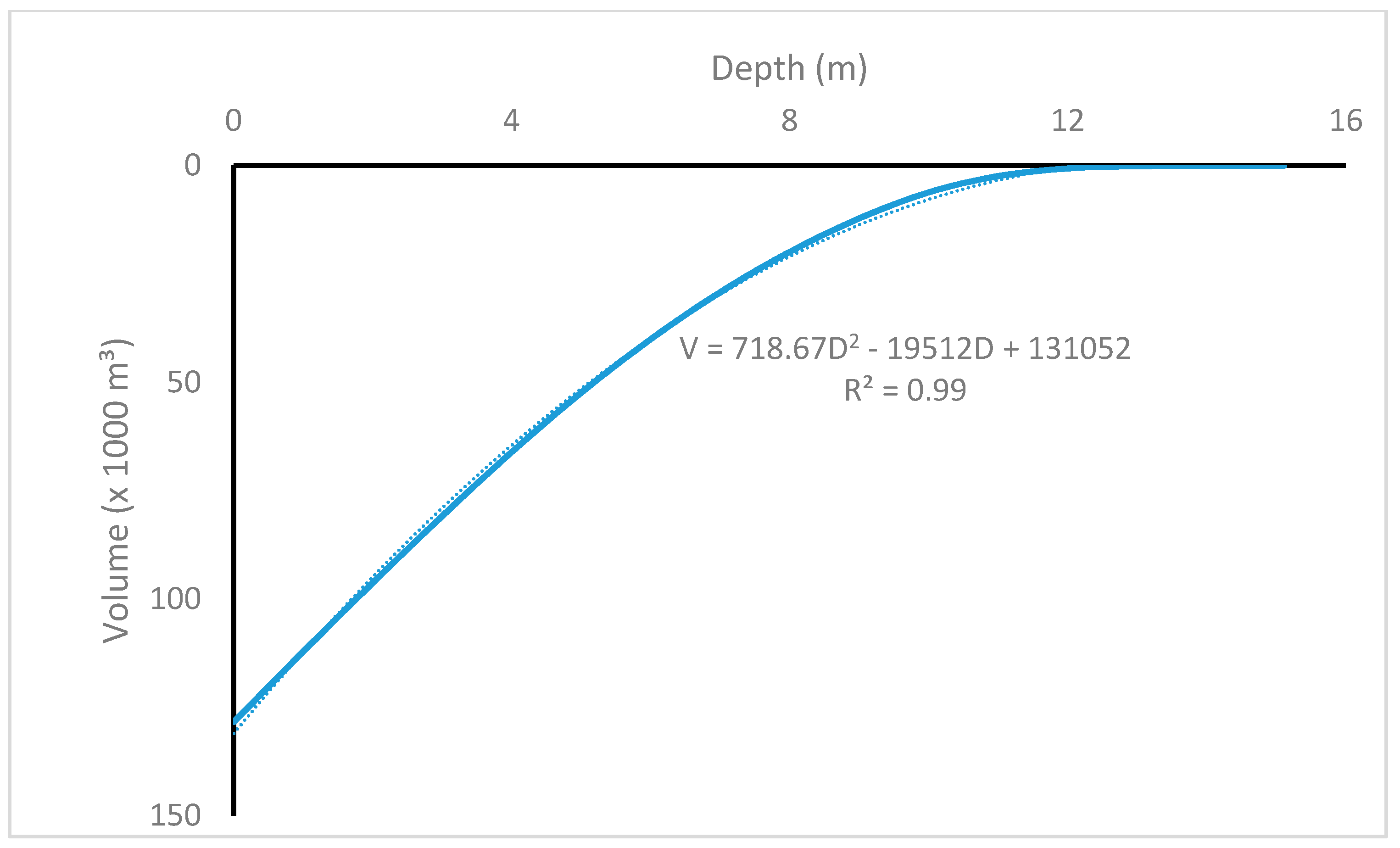
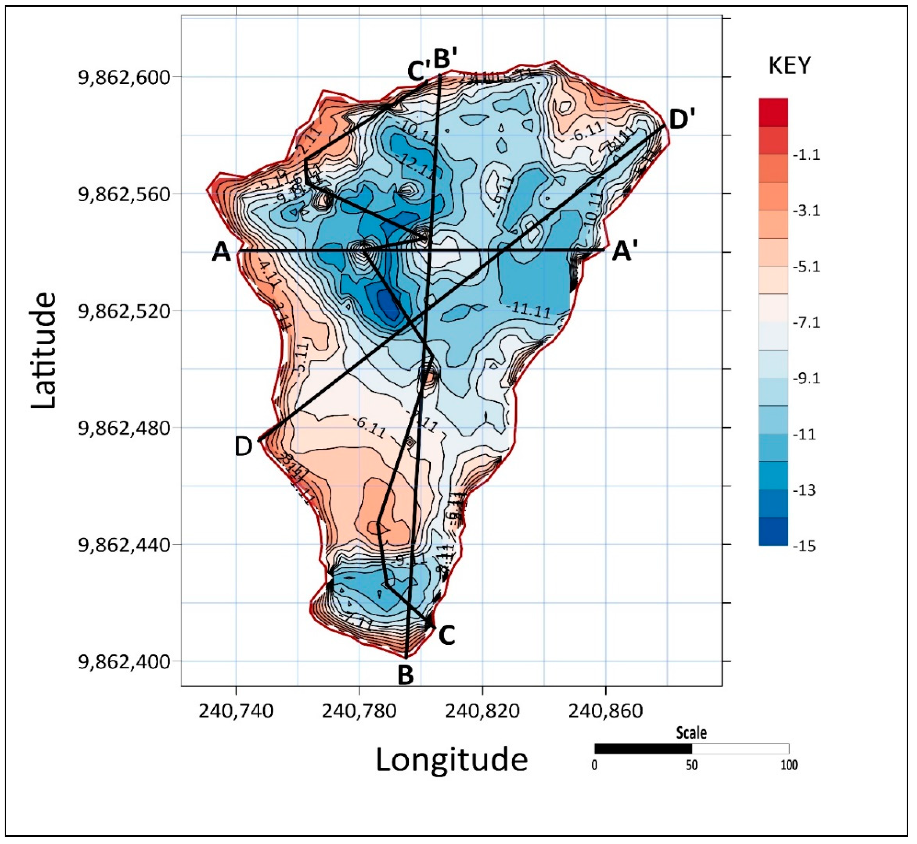
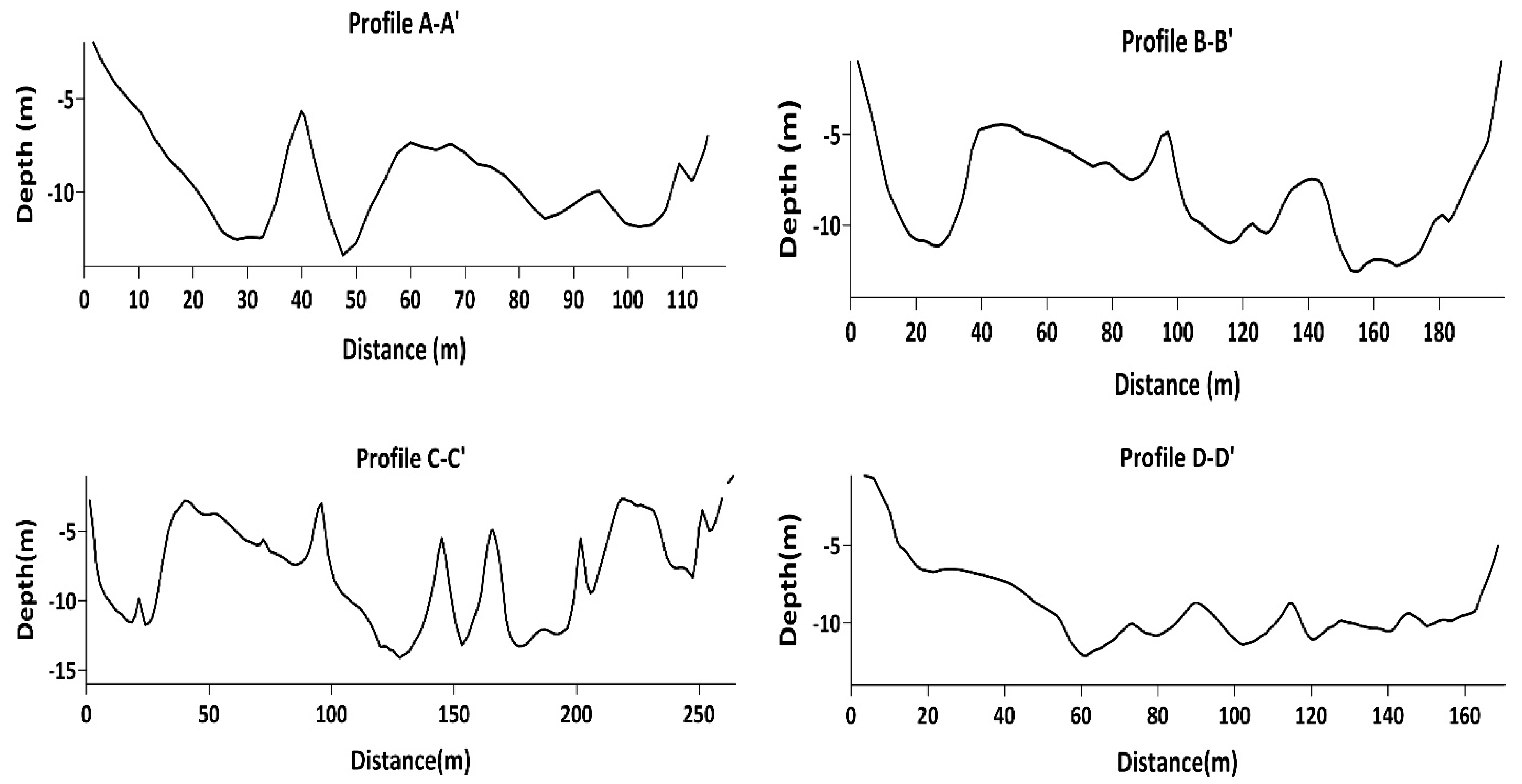
The study revealed that the storage capacity of the reservoir is 128,385 m³, the surface area is 17,699 m², the mean depth is 7.9 m, and the maximum depth is 15.11 m. This information is vital for assessing the water volume status at various stages, therefore enabling an informed decision to be made regarding the water withdrawal plan.

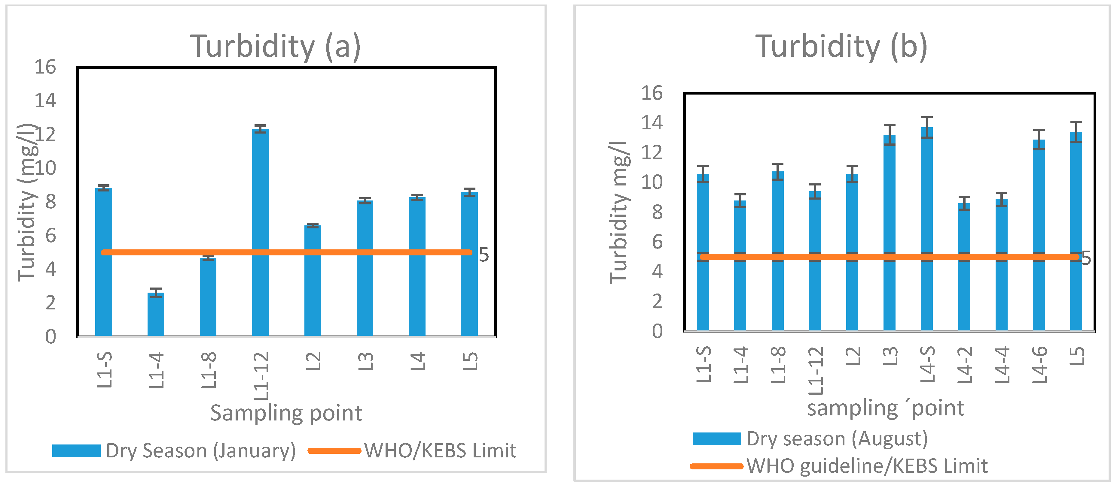
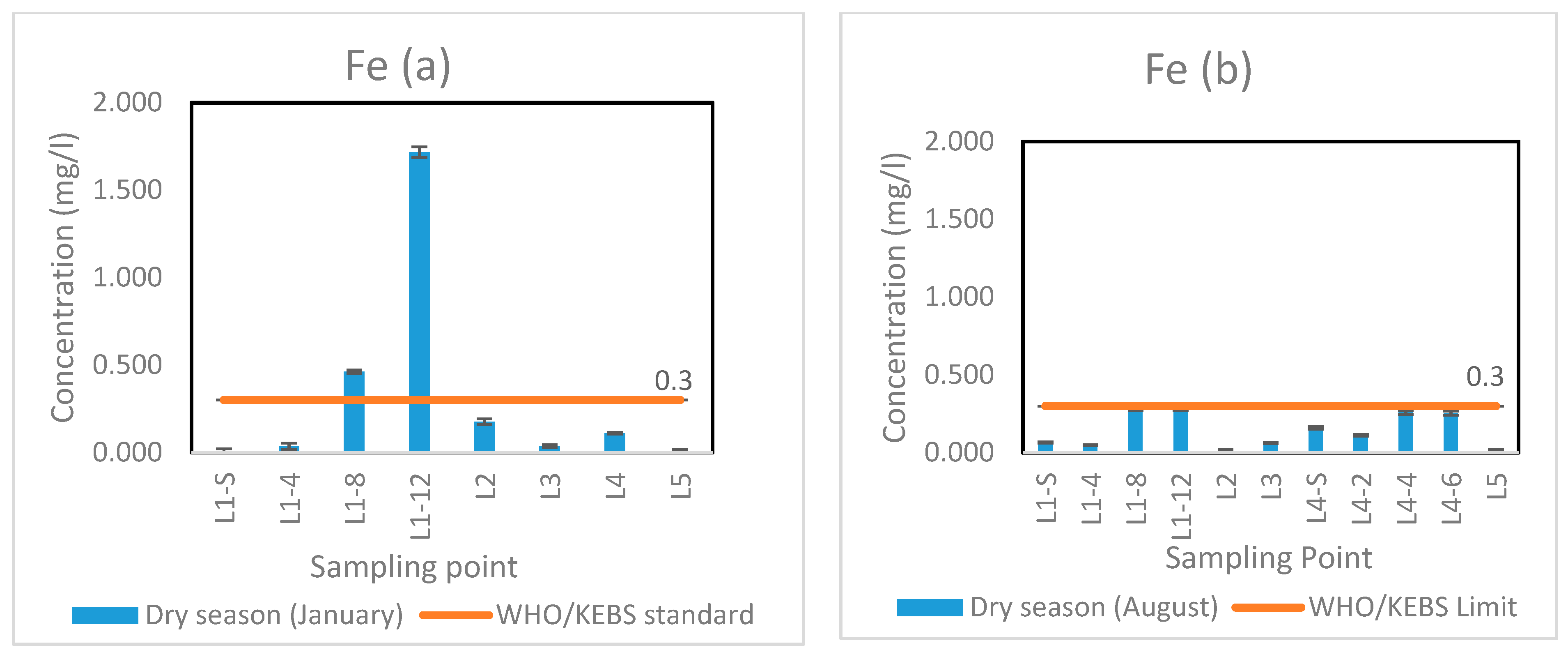
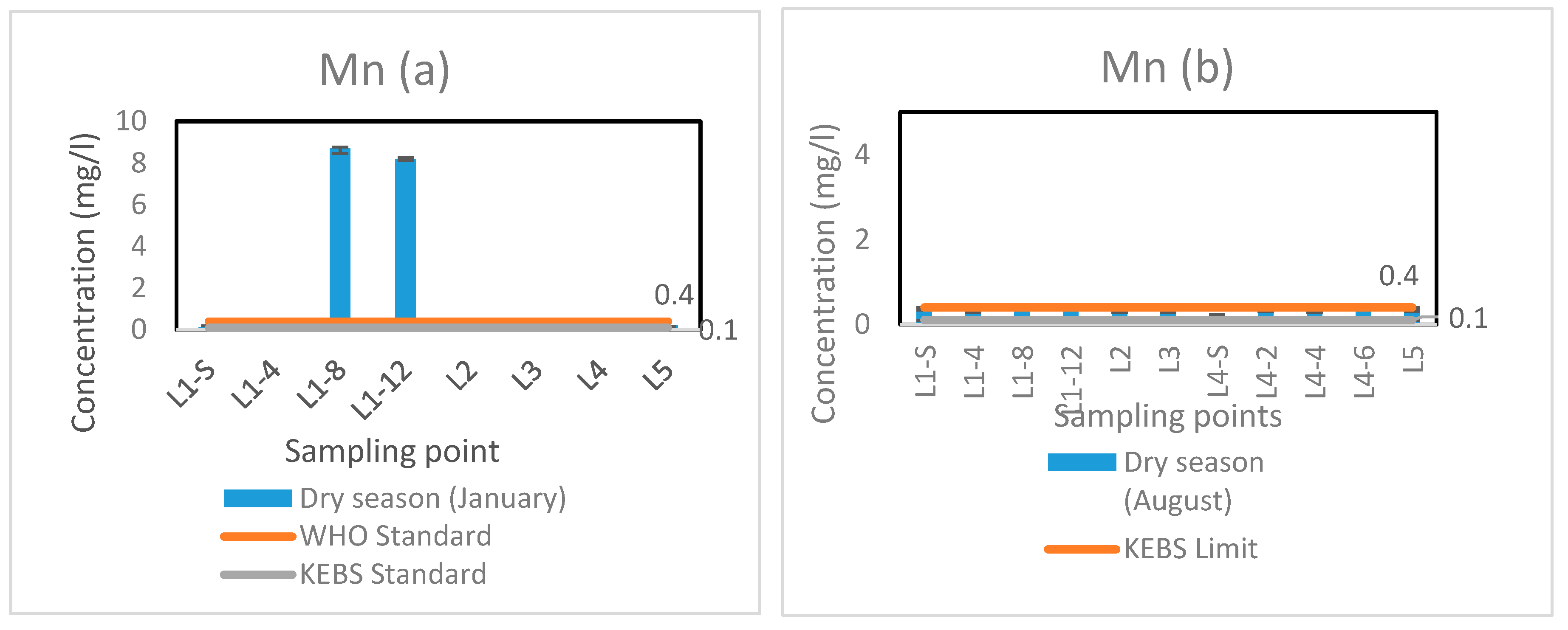
It was observed that except for cadmium, manganese, turbidity, and iron, which were above the maximum permissible limits, all water quality parameters in the reservoir were in compliance with WHO and KEBS standards. The bacteriological quality of the reservoir water was unacceptable and would pose a health risk to consumers if the water was consumed without treatment. The reservoir water is moderately soft, with mean cation and anion dominance in the order of Na > Mg > K > Ca and SO₄²⁻ > NO₃⁻ > NO₂⁻ > PO₄³⁻, respectively. Heavy metal dominance in the reservoir was in the order of Mn > Fe > Cu > Zn > Cr > Cd. Pb was not detected in the reservoir water. The mean concentrations of parameters were similar in January and August; however, most parameters had a higher concentration in August, especially Cadmium, as a result of the lower water level in the reservoir increasing the metal concentration in the liquid phase. During low input and evaporation in reservoirs, these values are expected to rise. Alternatively, in events of flooding, the volume of metals is expected to reduce because of dilution effect. From the computed WQI, the reservoir has a rating of good water quality. The water quality status during both sampling instances was similar, with WQI values of 83.31 in January and 85.85 in August.

The study recommends that the reservoir is fit as potential supplemental source of domestic water; however, treatment of the water is required before human consumption. Coagulation and filtration methods of treatment can achieve cadmium levels up to 0.002 mg/L [21,60]. Ion exchange, lime softening, and reverse osmosis are also approved by the Environmental Protection Agency (EPA) for cadmium removal. The other contaminants can be removed through conventional water treatment methods.

The main limitation of this study is failure to depict water quality during the rainy season because of inadequate rainfall. There was a constant decrease in water level in the reservoir during the study period. Comparison of water quality during dry and wet seasons is more informative in this study. A water quality model for forecasting water quality should be developed in future research. Also, comprehensive monitoring of water quality over the rainy season should be done.

References

1. Rathnayaka, K.; Malano, H.; Arora, M. Assessment of Sustainability of Urban Water Supply and Demand Management Options: A comprehensive approach. Water 2016, 8, 595. [Google Scholar] [CrossRef]
2. Favas, P.J.C.; Martino, L.E.; Prasad, M.N.V. Abandoned Mine Land Reclamation—Challenges and Opportunities (Holistic Approach); Elsevier Inc.: Amsterdam, The Netherlands, 2018; ISBN 9780128129869. [Google Scholar]
3. Antosch, L.M. Management of a Gravel-Pit Lake System to Optimize Future Water Quality. Ph.D. Thesis, Iowa State University, Ames, IA, USA, 1982. [Google Scholar]
4. Singleton, V.L.; Jacob, B.; Feeney, M.T.; Little, J.C. Modeling a Proposed Quarry Reservoir for Raw Water Storage in Atlanta, Georgia. J. Environ. Eng. 2013, 139, 70–78. [Google Scholar] [CrossRef]
5. Makanga, E.A.; Lomosi, M.A. Environmental Impact Assessment (EIA); Project Report for Proposed Kikuyu Water Supply Improvement Project: Nairobi, Kenya, 2015. [Google Scholar]
6. Athi Water Services Board. Multi Town Sustainable Water and Waste Water Management Program—Environmental and Social Impact Assessment Study; Kikuyu Sewerage Project: Nairobi, Kenya, 2016. [Google Scholar]
7. Fowe, T.; Karambiri, H.; Paturel, J.-E.; Poussin, J.-C.; Cecchi, P. Water balance of small reservoirs in the Volta basin: A case study of Boura reservoir in Burkina Faso. Agric. Water Manag. 2015, 152, 99–109. [Google Scholar] [CrossRef]
8. Ngugi, A. A Water Quality, Biodiversity Assessment and Community Perception Analysis of Rungiri Reservoir, Kikuyu Kenya. Master’s Thesis, University of Nairobi, Nairobi, Kenya, 2003. [Google Scholar]
9. Maina, C.W.; Sang, J.K.; Mutua, B.M.; Raude, J.M. Bathymetric survey of Lake Naivasha and its satellite Lake Oloiden in Kenya; using acoustic profiling system. Lakes Reserv. Res. Manag. 2018, 23, 324–332. [Google Scholar] [CrossRef]
10. Yesuf, H.M.; Alamirew, T.; Melesse, A.M.; Assen, M. Bathymetric study of Lake H ayq, Ethiopia. Lakes Reserv. Res. Manag. 2013, 18, 155–165. [Google Scholar] [CrossRef]
11. Ajith, A.V. Bathymetric Survey To Study The Sediment Deposit In Reservoir of Peechi Dam. J. Mech. Civ. Eng. 2016, 3, 34–38. [Google Scholar]
12. Curtarelli, M.; Leão, J.; Ogashawara, I.; Lorenzzetti, J.; Stech, J. Assessment of Spatial Interpolation Methods to Map the Bathymetry of an Amazonian Hydroelectric Reservoir to Aid in Decision Making for Water Management. ISPRS Int. J. Geo-Inf. 2015, 4, 220–235. [Google Scholar] [CrossRef]
13. Sang, J.; Maina, C. Generating multifunctional historical data for improved management of Reservoirs, Kenya. Sustain. Res. Eng. 2014, 3, 1–16. [Google Scholar]
14. Sima, S.; Tajrishy, M. Using satellite data to extract volume-area-elevation relationships for Urmia Lake, Iran. J. Gt. Lakes Res. 2013, 39, 90–99. [Google Scholar] [CrossRef]
15. Wu, C.-Y.; Mossa, J.; Mao, L.; Almulla, M. Comparison of different spatial interpolation methods for historical hydrographic data of the lowermost Mississippi River. Ann. GIS 2019, 25, 133–151. [Google Scholar] [CrossRef]
16. Sang, J.K.; Raude, J.M.; Mati, B.M.; Mutwiwa, U.N.; Ochieng, F. Dual Echo Sounder Bathymetric Survey for Enhanced Management of Ruiru Reservoir, Kenya. Sustain. Res. Eng. 2017, 3, 113–118. [Google Scholar]
17. Liebe, J.; van de Giesen, N.; Andreini, M. Estimation of small reservoir storage capacities in a semi-arid environment. Phys. Chem. Earth 2005, 30, 448–454. [Google Scholar] [CrossRef]
18. Aykut, N.O.; Akpınar, B.; Aydm, Ö. Hydrographic data modeling methods for determining precise seafloor topography. Comput. Geosci. 2013, 17, 661–669. [Google Scholar] [CrossRef]
19. Chukwu, F.N.; Badejo, O.T. Bathymetric Survey Investigation for Lagos Lagoon Seabed Topographical Changes. J. Geosci. Geomat. 2015, 3, 37–43. [Google Scholar]
20. Hickley, P.; Boar, R.R.; Mavuti, K.M. Bathymetry of Lake Bogoria, Kenya. J. East Afr. Nat. Hist. 2003, 92, 107–118. [Google Scholar] [CrossRef]
21. World Health Organisation. Guidelines for Drinking-Water Quality: Fourth Edition Incorporating the First Addendum; World Health Organisation: Geneva, Switzerland, 2017; ISBN 9241546964. [Google Scholar]
22. Chen, R.; Tsai, C. Development of an Evaluation System for Sustaining Reservoir Functions—A Case Study of Shiwen Reservoir in Taiwan. Sustainability 2017, 9, 1387. [Google Scholar] [CrossRef]
23. Schweitzer, L.; Noblet, J. Water Contamination and Pollution. In Green Chemistry; Elsevier: Amsterdam, The Netherlands, 2018; pp. 261–290. [Google Scholar]
24. WASREB. Drinking Water Quality and Effluent Monitoring Guideline; Water Services Regulatory Board: Nairobi, Kenya, 2006; pp. 1–36. [Google Scholar]
25. Cymes, I.; Szymczyk, S.; Glińska-Lewczuk, K.; Potasznik, A.; Cymes, I.; Sidoruk, M. Distribution and potential risk assessment of heavy metals and arsenic in sediments of a dam reservoir: A case study of the Łoje Retention Reservoir, NE Poland. J. Elem. 2017, 22, 843–856. [Google Scholar] [CrossRef]
26. Ashun, E.; Bansah, K.J. Groundwater quality index of Upper Athi River Basin in Kenya. Int. J. Glob. Environ. Issues 2017, 16, 217–230. [Google Scholar] [CrossRef]
27. Noori, R.; Berndtsson, R.; Hosseinzadeh, M.; Adamowski, J.F.; Abyaneh, M.R. A critical review on the application of the National Sanitation Foundation Water Quality Index. Environ. Pollut. 2019, 244, 575–587. [Google Scholar] [CrossRef]
28. Hussein, S.; Ali, S. Water quality index for Al-Gharraf River, southern Iraq. Egypt. J. Aquat. Res. 2017, 43, 117–122. [Google Scholar]
29. Al-mashagbah, A.F. Assessment of Surface Water Quality of King Abdullah Canal, Using Physico-Chemical Characteristics and Water Quality Index, Jordan. J. Water Resour. Prot. 2015, 7, 339–352. [Google Scholar] [CrossRef] [Green Version]
30. Alizadeh, M.J.; Kavianpour, M.R.; Danesh, M.; Adolf, J.; Shamshirband, S.; Chau, K.-W. Effect of river flow on the quality of estuarine and coastal waters using machine learning models. Eng. Appl. Comput. Fluid Mech. 2018, 12, 810–823. [Google Scholar] [CrossRef] [Green Version]
31. Shamshirband, S.; Jafari Nodoushan, E.; Adolf, J.E.; Abdul Manaf, A.; Mosavi, A.; Chau, K. Ensemble models with uncertainty analysis for multi-day ahead forecasting of chlorophyll a concentration in coastal waters. Eng. Appl. Comput. Fluid Mech. 2019, 13, 91–101. [Google Scholar] [CrossRef]
32. Abbasi, T.; Abbasi, S.A. Approaches to WQI Formulation. Water Qual. Indices 2012, 9–24. [Google Scholar] [CrossRef]
33. Bharti, N.; Katyal, D. Water quality indices used for surface water vulnerability assessment. Int. J. Environ. Sci. 2011, 2, 154–173. [Google Scholar]
34. Tyagi, S.; Sharma, B.; Singh, P.; Dobhal, R. Water Quality Assessment in Terms of Water Quality Index. Am. J. Water Resour. 2013, 1, 34–38. [Google Scholar]
35. Sidoruk, M.; Sidoruk, M. Effect of rainbow trout production in a two-stage cascade system on water quality. J. Elem. 2019, 24, 739–753. [Google Scholar] [CrossRef]
36. Sutadian, D. Development of a Cost Effective River Water Quality Index: A Case Study of West Java Province. Ph.D. Thesis, Victoria University, Melboune, Australia, 2017. [Google Scholar]
37. Brown, R.; McClelland, N.; Deininger, R.; Tozer, R. A-Water-Quality-Index-Do-We-Dare. Water Sewage Works 1970, 117, 339–343. [Google Scholar]
38. Cude, C.G. Oregon water quality index a tool for evaluating water quality management effectiveness. J. Am. Water Resour. Assoc. 2001, 37, 125–137. [Google Scholar] [CrossRef]
39. Mumma, A.; Lane, M.; Kairu, E.; Tuinhof, A.; Hirji, R. Kenya Ground Water Governance Case Study; The Water Unit, Transport, Water and ICT Department: Washington DC, USA, 2011. [Google Scholar]
40. Rousakis, G.; Panagiotopoulos, I.P.; Drakopoulou, P.; Georgiou, P.; Nikolopoulos, D.; Mporompokas, N.; Kapsimalis, V.; Livanos, I.; Morfis, I.A.; Anagnostou, C.; et al. Sustainability evaluation of Mornos Lake/Reservoir, Greece. Environ. Monit. Assess. 2018, 190, 64. [Google Scholar] [CrossRef]
41. Texas Water Development Board. Bathymetric survey of the West Fork San Jacinto River; Texas Water Development Board: Austin, TX, USA, 2018. [Google Scholar]
42. Arroyo Environmental Consultants, LLC. Volumetric and Sedimentation Study on Wright Patman Lake; Riverbend Water Resources District: New Boston, TX, USA, 2019. [Google Scholar]
43. Bezerra-Neto, J.F.; Briguenti, L.S.; Pinto-Coelho, R.M. A new morphometric study of Carioca Lake, Parque Estadual do Rio Doce (PERD), Minas Gerais State, Brazil. Acta Sci. Biol. Sci. 2010, 32, 49–54. [Google Scholar] [CrossRef]
44. APHA. Standard Methods for the Examination of Water and Wastewater; American Public Health Association, American Water Works Association, Water Environment Federation: Washngton, DC, USA, 2012. [Google Scholar]
45. Adimalla, N.; Qian, H. Groundwater quality evaluation using water quality index (WQI) for drinking purposes and human health risk (HHR) assessment in an agricultural region of Nanganur, south India. Ecotoxicol. Environ. Saf. 2019, 176, 153–161. [Google Scholar] [CrossRef] [PubMed]
46. Hameed, A.; Alobaidy, M.J.; Abid, H.S.; Maulood, B.K. Application of Water Quality Index for Assessment of Dokan Lake Ecosystem, Kurdistan Region, Iraq. J. Water Resour. Prot. 2010, 2010, 792–798. [Google Scholar]
47. RadFard, M.; Seif, M.; Ghazizadeh Hashemi, A.H.; Zarei, A.; Saghi, M.H.; Shalyari, N.; Morovati, R.; Heidarinejad, Z.; Samaei, M.R. Protocol for the estimation of drinking water quality index (DWQI) in water resources: Artificial neural network (ANFIS) and Arc-Gis. MethodsX 2019, 6, 1021–1029. [Google Scholar] [CrossRef] [PubMed]
48. Sisay, T.; Beyene, A.; Alemayehu, E. Journal of Environmental Science and Pollution Research Assessment of Drinking Water Quality and Treatment Plant Efficiency in Southwest Ethiopia. J. Environ. Sci. 2017, 3, 208–212. [Google Scholar]
49. Bhat, S.A.; Pandit, A.K. Surface Water Quality Assessment of Wular Lake, a Ramsar Site in Kashmir Himalaya, Using Discriminant Analysis and WQI. J. Ecosyst. 2014, 2014, 724728. [Google Scholar] [CrossRef]
50. Prasad, M.; Sunitha, V.; Reddy, Y.S.; Suvarna, B.; Reddy, B.M.; Reddy, M.R. Data in brief Data on water quality index development for groundwater quality assessment from Obulavaripalli Mandal, YSR district, AP India. Data Br. 2019, 24, 103846. [Google Scholar] [CrossRef]
51. Explosives and Aggregate. Available online: https://www.dnr.illinois.gov/mines/EAD/Pages/FAQAgreggateBlasting.aspx#qst4 (accessed on 22 July 2019).
52. Woldeab, B.; Beyene, A.; Ambelu, A.; Buffam, I.; Mereta, S.T. Seasonal and spatial variation of reservoir water quality in the southwest of Ethiopia. Environ. Monit. Assess. 2018, 190, 163. [Google Scholar] [CrossRef]
53. Salari, M.; Salami, E.; Afzali, S.H.; Ehteshami, M.; Conti, G.O.; Derakhshan, Z.; Sheibani, S.N. Quality assessment and artificial neural networks modeling for characterization of chemical and physical parameters of potable water. Food Chem. Toxicol. 2018, 118, 212–219. [Google Scholar] [CrossRef]
54. Daghara, A.; Al-Khatib, I.A.; Al-Jabari, M. Quality of Drinking Water from Springs in Palestine: West Bank as a Case Study. J. Environ. Public Health 2019, 2019, 8631732. [Google Scholar] [CrossRef]
55. Pippa, J.C.; Paul, K.; Gordon, N.M.; Pitts, C. Surface Water Quality. In Water Resources: An Integrated Approach; Holden, J., Ed.; Routledge: London, UK, 2013; pp. 79–122. ISBN 0415602823. [Google Scholar]
56. Ling, T.-Y.; Gerunsin, N.; Soo, C.-L.; Nyanti, L.; Sim, S.-F.; Grinang, J. Seasonal Changes and Spatial Variation in Water Quality of a Large Young Tropical Reservoir and Its Downstream River. J. Chem. 2017, 2017, 8153246. [Google Scholar] [CrossRef]
57. Environmental Protection Agency. Parameters of Water Quality; Environmental Protection Agency: Wexford, Irelnd, 2001.
58. Kulinkina, A.V.; Plummer, J.D.; Chui, K.K.H.; Kosinski, K.C.; Adomako-Adjei, T.; Egorov, A.I.; Naumova, E.N. Physicochemical parameters affecting the perception of borehole water quality in Ghana. Int. J. Hyg. Environ. Health 2017, 220, 990–997. [Google Scholar] [CrossRef] [PubMed]
59. Mustapha, M.K.; Wulum, J.C. Seasonal assessment, treatment and removal of heavy metal concentrations in a tropical drinking water reservoir. Ekol. Bratislava 2016, 35, 103–113. [Google Scholar] [CrossRef] [Green Version]
60. Eliku, T.; Leta, S. Spatial and seasonal variation in physicochemical parameters and heavy metals in Awash River, Ethiopia. Appl. Water Sci. 2018, 8, 177. [Google Scholar] [CrossRef] [Green Version]
Figure 1. Location map of the study area.
Hydrology 06 00093 g001
Figure 2. Bathymetry survey equipment set up.
Hydrology 06 00093 g002
Figure 3. Rungiri quarry reservoir sampling points.
Hydrology 06 00093 g003
Figure 4. Depth–volume relationship for Rungiri quarry reservoir.
Hydrology 06 00093 g004
Figure 5. Depth–surface area relationship for Rungiri quarry reservoir.
Hydrology 06 00093 g005
Figure 6. Depth contours of Rungiri quarry reservoir.
Hydrology 06 00093 g006
Figure 7. Depth profiles of Rungiri quarry reservoir.
Hydrology 06 00093 g007
Figure 8. Turbidity concentration at various sampling points: (a) January 2019 and (b) August 2019.
Hydrology 06 00093 g008
Figure 9. Iron concentration at various sampling points during the dry season: (a) January and (b) August.
Hydrology 06 00093 g009
Figure 10. Cadmium concentration at various sampling points during the dry season: (a) January and (b) August.
Hydrology 06 00093 g010
Figure 11. Manganese concentration at various sampling points: (a) January and (b) August.
Hydrology 06 00093 g011