1. Introduction
Sierra Nevada is an abrupt and relatively small (179,000 ha) but high (3479 m a.s.l.) massif, located in the western region of the Mediterranean basin (
Figure 1). In 1986, the central nucleus of this massif was declared Reserve of the Biosphere [
1] and it is one of the 25 biodiversity hot spots [
2,
3,
4]. However, usually the content receives more attention than the container, disregarding the high degree of dependence between biota and physical substratum, both with similar risks for their subsistence.
This is the case of the water-bodies scattered over the Sierra Nevada massif. These biotopes are of particular interest, as they are located at altitude, in niches unique in Europe, under severe conditions, exposing the vegetation to stressful climatic regimes, which differ depending on whether exposure is northerly or southerly. These scenarios encourage the delicate development of water-bodies, making them particularly sensitive to present climatic changes.
A general characteristic of these water-bodies is their small size, i.e., small lakes, pools, ponds, fens, etc. They are fed by snowmelt, many are short-lived, and occasionally they are surrounded by a peripheral fringe of herbaceous vegetation (hereafter green fringes). In contrast to the extreme aridity of the surrounding landscape, these water-bodies resemble oases, thereby being of value and worthy of being protected, although they are still scarcely studied. In agreement with Alvarez-Cobelas et al. [
5], we can say that because of these specific features there is a need to establish a Mediterranean limnology paradigm.
The Mediterranean basin is the only region on Earth affecting three continents, whose transboundary limits cover over 10
7 km
2 [
6]. It is, therefore, a zone of convergence and interaction, with heterogeneous features [
7]. Although the Mediterranean mountain environments have been studied in the literature (e.g., [
8,
9,
10]), there is still a lack of studies focusing on diverse aspects of the hydrological cycle, particularly those related with the medium and long term water regime, and especially the relations between ice, water and the subsidiary green fringes.
We specifically address the following points: (1) the main volumetric components of the hydrological cycle in the studied setting. (2) The annual timing of the thaw. (3) The distribution of water-bodies on the two main watersheds, considering the higher xericity of one against the other. (4) The noteworthy presence of green fringes and their dependence on water-bodies on both watersheds.
Although a key problem in many parts of the semiarid Mediterranean is the absence of reliable, long-term records of river flows [
11], we are able to answer such questions because the area in question has a water reservoir provided with suitable monitoring equipment, as well as good aerial documents and it is suitably sized.
2. Materials and Methods
2.1. Study Area
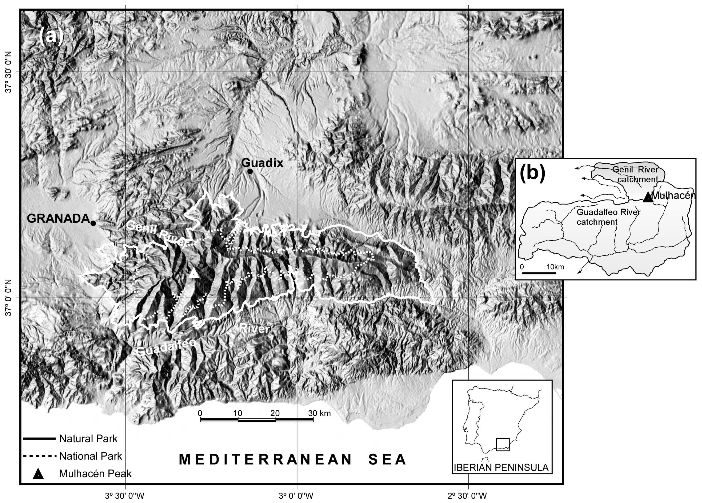
The Sierra Nevada massif (
Figure 1a and
Figure 2a) is located in the SE of the Iberian Peninsula. The Mulhacén is the highest peak (3479 m a.s.l.,
Figure 2b), which makes this the second highest massif in Western Europe, after Mont Blanc (4810 m a.s.l.) in the Alps.
The surface studied extends over approximately 30 km maximum length (E–W, Caballo–Veleta–Mulhacén–Cerro Pelado peaks) and maximum width of 20 km, giving an area of some 170 km
2 with altitudes over 2480 m a.s.l. The water-bodies are near the highest peaks, above 2700 m a.s.l. Two main catchments determine the hydrology (
Figure 1b): that of the Genil River (Atlantic watershed) and that of the Guadalfeo River (Mediterranean watershed). Protected species were at no time put at risk by the work involved in this study.
The rocks of Sierra Nevada belong to the innermost units of the Betic Cordilleras (SE Spain) [
12,
13,
14] consisting of a monotonous sequence of graphite-bearing metapelites with intercalated quartzite, and some marble and other metamorphic rocks; they constitute more than 90% of the outcrops in the western Sierra Nevada and are several kilometers thick [
15].
There are also more recent features, viz. moraines, glacial–fluvial deposits, rock glaciers, gelifluction soils, debris cones and blockfields [
16]. They are detritic in nature, accumulated as irregular, epidermal deposits by the activity of Quaternary glaciers.
General speaking, all the water-bodies studied are mainly related to the latter features, and their permanence depends on the seepage rate through the rocks. In addition, alteration phenomena of rocky substrates determine regolith in a variable band of altitude where the annual effects of successive ice-thaw cycles accumulate. Water-bodies are mainly originated by glacier overdeepening phenomena and some of them are damned by rocky thresholds or moraine deposits. Some of these deposits testify to glacial activity in Sierra Nevada during the last cold periods of the Pleistocene [
17,
18], but these glaciers were never as significant as in more northern cordilleras (Pyrenees, Alps), and are no longer present [
10,
19]. Snow cover is now seasonal and associated with nival processes.
The water-bodies studied present a wide range of shallow morphologies (
Figure 2c–f) typical of this massif within the cryo–oromediterranean (or Alpine) level. Several studies have showed that the sediments filling these depressions are Holocene, although there is a time difference between them [
20,
21].
Sierra Nevada constitutes perhaps the set of ecosystems most representative of Mediterranean high mountains, with an extreme southern location on the European continent and characterized by a climate of not excessively low winter temperatures and strong summer xericity.
Table 1 summarizes data from three meteorological stations in the area. In addition, each of the valleys and associated ravines and water courses show microclimatic differences, as well as changes in insolation on slopes.
Bioclimatic classifications [
24,
25] recognize the relationship between vegetation and climate. The type of vegetation in the study area corresponds to an oromediterranean belt (2000–2900 m a.s.l.; creeping juniper and savin juniper groves) and a cryo–oromediterranean belt (>2900 m a.s.l.; high mountain). Both belts are the Mediterranean equivalents of the Sub-Alpine and Alpine zones [
26] and contain most of the endemic species [
27] and water-bodies. Part of the study area could be ascribed to a biogeographical unit [
28], but the reality is rather heterogenous, with a notable diversity of environments depending on factors such as altitude, slope, soils or humidity.
2.2. Methods
Visits were scheduled to every wetland in the area after the thaw over a long enough period to include wet and dry years (2000–2017). The water-bodies were identified on a 1:25.000 topographical map [
29], on the geomorphological map of Sierra Nevada [
16] and on black and white digital orthophotos (1:20.000) by the regional government (Junta de Andalucía). This was completed by an exhaustive exploration of new water-bodies not recorded on previous documents. We also used Google Earth Digital Globe imagery [
30] to detail the water-bodies’ geographic position in Sierra Nevada. The Iberpix visualizer [
31] allowed us to exchange cartographic and land-image information. These tools were used to estimate elevations and measure the size and area of each water-body. In any case, the absolute altitudes are based on data from National Topographical Maps 1:25.000 [
29]. Measurements were made on orthogonal images at water surface level to minimize distortions. The cartography was based on images mainly recorded in the summer of 2015. Old aerial photographs (B&W) were also used to estimate some features for specific natural water-bodies, such as Laguna de las Yeguas, due to the effects of man-made changes to build a dam for a reservoir.
During the field study we photographed and measured each water-body and its associated details (
Figure 2 and
Figure 3). We likewise collected geographical information (altitude and UTM coordinates using GPS) and quantitative data (length, width and maximum water depth, using a tape-measure and a single-seat rubber boat). A few temporary water-bodies were detected by the presence of sediments or thin coatings on rocks, presumably formed in hollows (
Figure 3a), and also by occasional associated green fringes (
Figure 2c–f): these cases were revisited in wetter years for confirmation. In addition, we often detected horizontal lines on the rocks at the edges as indications of the maximum level of the water-sheet, and which we have used as indicators of water “historic-levels” (
Figure 3b,c). Other data on the water-bodies concerned the presence/absence of glacial action, morphology of the basins, presence/absence of green fringes, types of floors (sandy, loamy, rocky), presence of springs, and influents/effluents. All the information was stored in a database and general or detailed cartography was performed as appropriate.
Water volume was calculated by using the surface area of the water sheets (S
w) at their maximum, as mapped from highly magnified aerial photographs. This maximum was accurately assessed in the water-bodies with green fringes by markings usually found around the edge. There was good agreement between photogrammetry data and field measurements (R
2 = 0.918,
p < 0.000). Once the area was obtained, the volume of each water-body was calculated applying the cylinder (1), ½ ellipsoid (2) or cone (3) formulas, depending on whether they were respectively <0.5 m, 0.5–2 m, or >2 m deep (h= depth of the water sheet). We consider that these are the maximum volumes of water retained in the systems. In addition, we estimated water volumes draining towards the north-facing slope of this massif during the period 2000–2017. We collected flow-rate data from the Canales reservoir (Genil River, UTM: 457418mE-4112671mN, 959 m a.s.l., Atlantic watershed) from the Automatic Hydrological Information System [
22]. The watershed of the Canales reservoir is 176 km
2 in area, of which 60 km
2 (34%) lie between 2200 and 3479 m a.s.l., mostly corresponding to the surface covered by snow from November to June. Its substratum consists mainly of micaschists and quartzites. Hydrogeological interferences and an incomplete monitoring network made it hard to estimate volumes draining towards the southern watershed of the massif.
3. Results
We analyzed the factors affecting the water supply, the hydrological dependence of these water-bodies, and their spatial distribution and size based on the study of the different characteristics of 123 water-bodies distributed throughout this massif (
Figure 4).
3.1. Distribution and General Characteristics of Water-Bodies
3.1.1. Distribution of Water-Bodies
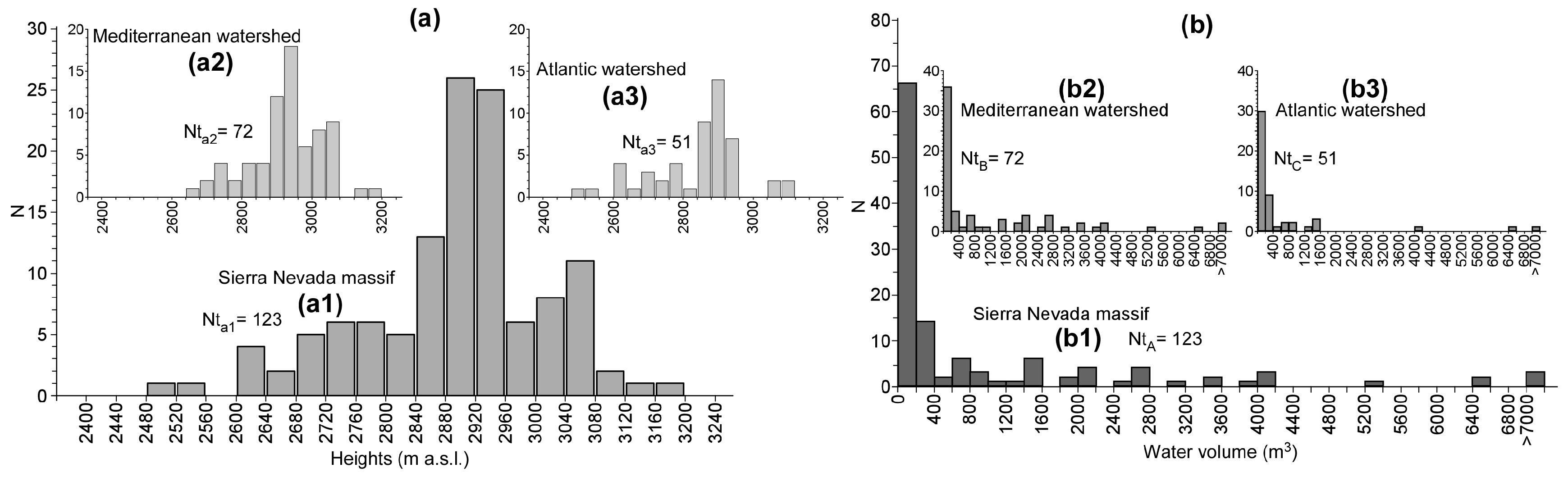
The distribution of water-bodies by altitude shows two clear maxima (
Figure 5(a1)). The best defined range lies between 2880 and 2960 m a.s.l. (51% of cases), while the second maximum covers the 3000–3080 m a.s.l. range (19% of cases). Both situations correspond to areas that remain covered by snow for most of the year, even in years when precipitation is low. A third maximum is found between 2720 and 2800 m a.s.l. (12%), but is less well defined. This area is located in zones close to the continuous oscillations observed every year in the snow level, even in years of abundant precipitation. In short, 90% of the water-bodies are found above 2700 m a.s.l.
Since the line of peaks runs E-W along the massif (
Figure 1 and
Figure 4), there is a clear definition of the northern (Atlantic basin) and southern (Mediterranean basin) watersheds. In principle, this could encourage the accumulation and permanence of snow on one watershed more than the other, and so both must be differentiated in this analysis. It is striking that the breakdown of data by watershed (
Figure 5(a2,a3)) shows the largest number of water-bodies on the Mediterranean watershed, which has lower mean annual precipitation (see
Table 1). On the Mediterranean watershed, 30 of the 72 water-bodies are found between 2880 and 2960 m a.s.l. (24% of the water-bodies on the massif), 17 form the second maximum (3000 to 3080 m a.s.l., 14%) and 17 are found in the 2640–2880 m a.s.l. range (14%). The 51 water-bodies of the Atlantic watershed are mainly concentrated between 2840 and 2960 m a.s.l. (30 water-bodies, representing 24% of the total on the massif), and the rest are found at lower altitudes. Below 2700 m a.s.l. only 3 water-bodies are on the Mediterranean watershed and 10 on the Atlantic. In other words, the water-bodies of the Mediterranean watershed are concentrated at altitudes above 2880 m a.s.l. (38%) and have a more structured distribution than those on the Atlantic watershed. The altitude range of the maximum accumulation of water-bodies is relatively similar in both cases.
3.1.2. Hydrological Relation between Water-Bodies
In the various sub-basins there are water-bodies that receive snowmelt and transmit it to each other by means of connecting watercourses (
Figure 4). Just towards the end of the true thaw, the detrital surface covering (including the soil itself) is saturated, and supplies the water exceeding its retention capacity as the sub-surface volume (Ss). Some examples are the Lagunillos de la Virgen (higher and lower), Laguna del Carnero and Laguna Hondera. When this supply ceases, the watercourses cease to flow from the upper water-body to the lower. The water then lies on the water-bodies and undergoes evapotranspiration and/or infiltration, the pastures dry up and Sierra Nevada slowly becomes more arid.
As stated before (
Section 3.1.1), the line of the Sierra Nevada peaks divides the massif into two watersheds facing north and south. As is generally true of the northern hemisphere, the northern orientation of the Atlantic sub-basins leads to longer lying snow on the slopes [
32,
33,
34,
35]. On the contrary, the southern orientation of the Mediterranean watershed provides a higher number of freeze-thaw cycles throughout the year because it has higher insolation. These slopes therefore have higher potential for alteration of the geological substratum, i.e., higher development of the regolith, as well as lower permanence of snow cover.
Table 2 summarizes the main characteristics of all the headwaters studied. The Atlantic watershed has 7 headwaters and the Mediterranean 10. These headwaters have been determined as the area including various sets of water-bodies from a maximum altitude of never less than 3000 m a.s.l. to a minimum altitude of 2500 m a.s.l., with some exceptions. The dimensions range from 1.0 km
2 for the Valdecasillas headwaters (seven water-bodies) to the 13.1 km
2 of the headwaters of the Dílar River (twenty-two water-bodies) whose size is linked to the lowest water-bodies studied (2498 m a.s.l.). We observed that the largest specific surfaces (perimeter/surface quotient) progressively increased in size at 2500, 2700 and 2900 m a.s.l. The overall values of the Mediterranean watershed are higher than those of the Atlantic watershed in all characteristics, and the area of green fringes associated with the water-bodies of the Mediterranean watershed is almost five times larger.
3.1.3. Characteristics of Water-Bodies
3.1.3.1. Morphologies and Sizes
In plain view, most of the water-bodies have pseudo-elliptical shapes, and rarely geometrical, anastomosed or a mixture of both shapes.
We define the area of the water-bodies as the surface of the water sheet at the highest melt point (normally in June). The largest surface area on the Atlantic watershed belongs to Laguna Larga (21,117 m2), and on the Mediterranean watershed it is Laguna de la Caldera (11,630 m2). The surface of the water sheet is less than 1000 m2 in 54% of the water-bodies, while it is over 5000 m2 in 4%.
Water depth varies, at the highest melt point, from 11.0 m in Laguna de la Caldera to 0.2 m for many water-bodies (mean value 1.1 m). The deepest are of glacial origin (Vacares, 8.8 m; Larga, 7.1 m, among others) and are located at high altitude (>2700 m). Other water-bodies have less depth, despite their glacial origin (La Mosca, 3.3 m; Corral del Veleta, 2.6 m, among others). Many water-bodies are shallow and closely linked with green fringes. These water-bodies are unevenly distributed by watersheds (
Figure 4).
We should also mention fifteen other areas appearing as clusters of small pools, sometimes consisting of up to 100 individual elements, almost all less than 1 m2 in area, around 25 cm deep and surrounded by abundant hygrophilous vegetation. These cases have not been considered as water-bodies in the present study.
3.1.3.2. Water Volumes Stored in the Water-Bodies
We should point out that the volume of water stored in these water-bodies remains constant until supply ceases at the end of the thaw, when it gradually decreases through evapotranspiration and/or infiltration and sub-surface supply does not provide substantial stability to the volume present. This phenomenon occurs every year, varying in intensity according to the annual pluviometric record, the amount of snow accumulated in the headwaters and the degree of summer drought, which can cause the functional disappearance of the water-bodies as such, until the next period of rainfall.
The distribution of the estimated volumes for these water-bodies on the entire massif (
Figure 5(b1)) show that there are an important number of water-bodies of less than 1000 m
3 (93 cases, 76% of the total), whereas there are only six cases of water-bodies over 5000 m
3 (5%): Laguna Larga (50,000 m
3), Caldera (42,500 m
3), Vacares (23,800 m
3), Caballo (6400 m
3), Mosca (6400 m
3) and Altera (5400 m
3), in decreasing order of magnitude. The volume of water contained in total is approximately 215,000 m
3, and the volume contained in those of more than 5000 m
3 totals 134,500 m
3, i.e., 66% of the content throughout the massif. The surface occupied is around 170,000 m
2.
The distribution by watersheds presents a similar pattern (
Figure 5(b2,b3)). However, we observed that the Mediterranean watershed contains 53 water-bodies of less than 2000 m
3 (18,000 m
3 total), 16 bodies in the 2000–6000 m
3 range (50,200 m
3) and three bodies over 6000 m
3 (73,000 m
3), whereas on the Atlantic watershed there are 48 water-bodies smaller than 2000 m
3 (14,000 m
3 total), only one body in the 2000–6000 m
3 range (4100 m
3) and two over 6000 m
3 (56,000 m
3). In total, the water-bodies on the Mediterranean watershed store 140,000 m
3 and those on the Atlantic watershed 75,000 m
3.
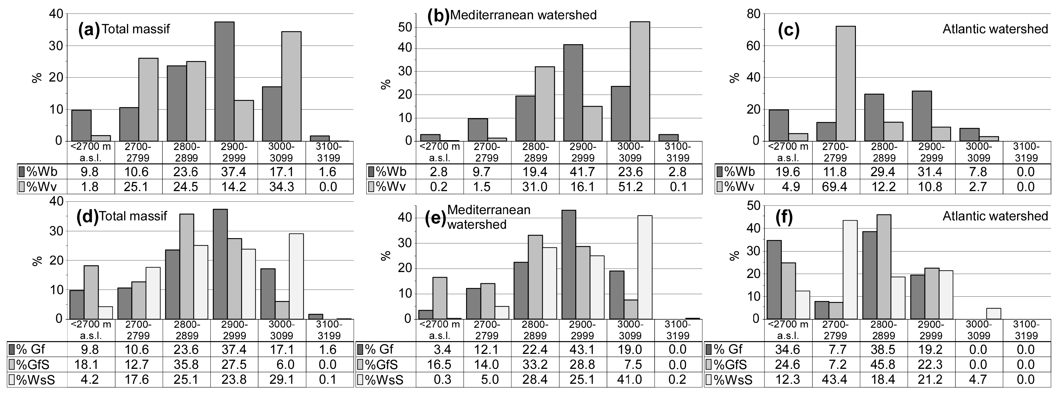
Finally, we can consider the relations between the number of water-bodies, their volume and altitude (100 m intervals). The highest number of water-bodies throughout the massif is found between 2900 and 3000 m a.s.l. (37%) (
Figure 6a), although the maximum volume (34%) is between 3000 and 3100 m a.s.l. because of their size. The number of water-bodies falls considerably above 3100 m, and both variables are balanced between 2800 and 2900 m a.s.l. (24%). These general characteristics are to a large extent the result of the conditions of the water-bodies on the Mediterranean watershed (
Figure 6b), where the maximum number is between 2900 and 3000 m a.s.l. (42%) and just over 50% of the water volume is between 3000 and 3100 m a.s.l. But the case is different for altitudes below 2800 m a.s.l., where the Atlantic watershed (
Figure 6c) has a lower number of water-bodies (12%) between 2700 and 2800 m a.s.l., whose volume represents 70% of the total storage on this watershed.
3.2. Hydrology
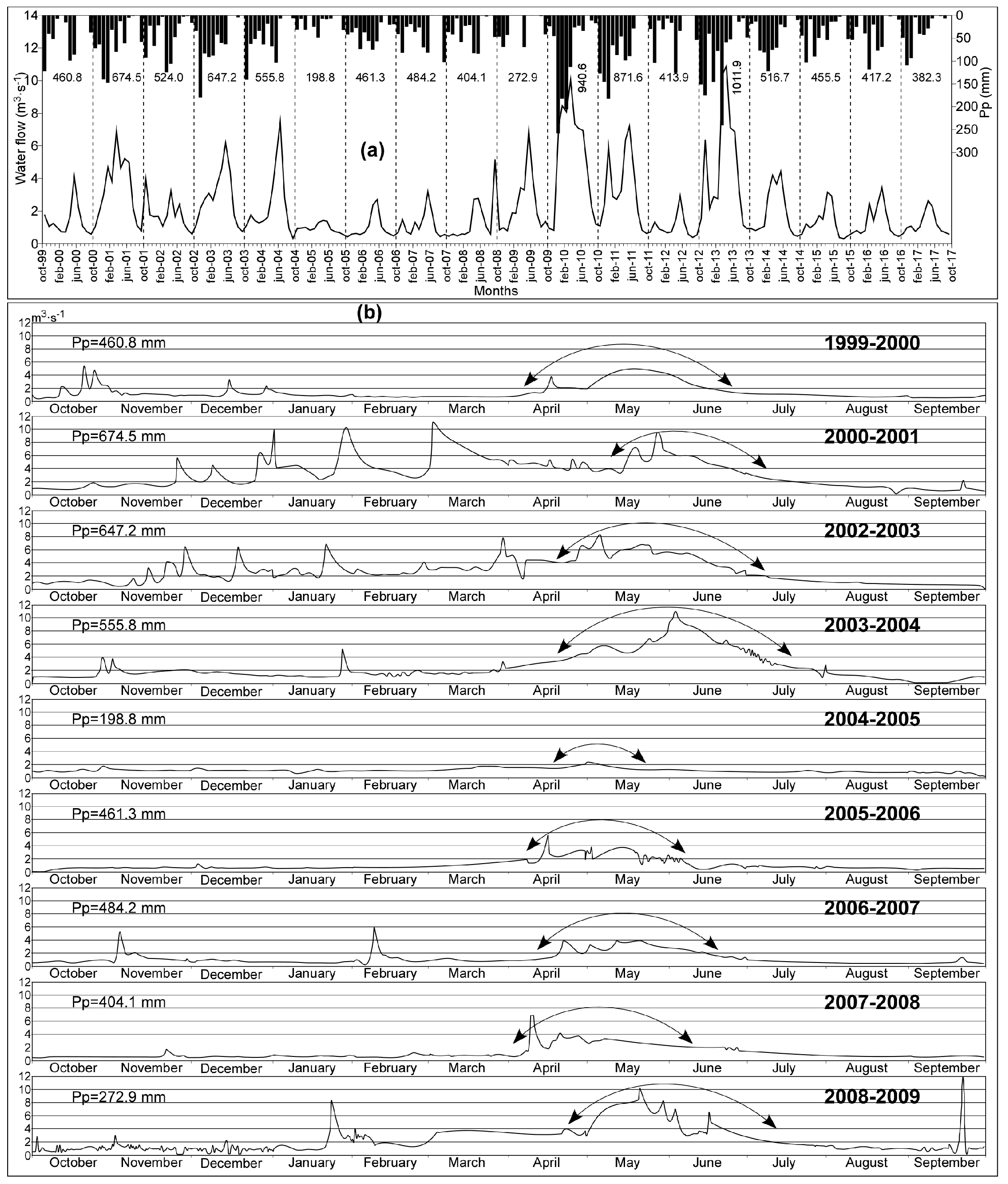
Hydrological characteristics were established on the basis of rainfall and water-flow data from the Canales hydrological station (headwaters of the Genil River) throughout the study period (1999–2017). Rainfall (
Figure 7a, upper vertical bars) shows considerable year-to-year variations, with values between 198.8 and 1011.9 mm and a mean value of 538.5 mm, with rainy winters and dry summers each year, as well as increased precipitation in 2010–2013. The gradual decrease in precipitation of the last four years is also noticeable. Flow-rate (
Figure 7a, continuous line) shows a succession of peaks and troughs corresponding to the rainfall bars, and follows the patterns of low (hydrological years 2004–2007 and 2014–2017) and higher precipitations (2009–2010 and 2012–2013). We point out that each year: (1) highest water-flow occurred in May and June, and (2) there was a lag between maximum precipitation and maximum water-flow, although the monthly data are not sensitive enough to show this causal relation. So we have made use of hourly data (hydrograms in
Figure 7b). These data are also from the Canales station, and only the 2000–2009 period has data without defects in the records. The snow of the peaks gradually melts from June onwards until disappearing completely. The thaw period varied according to the winter precipitations and depth of snow accumulated, sometimes lasting until August, and the water-bodies fill during this period. Arrows represent the moments of maximum water flow coinciding with periods of strongest thaw. This is best defined for the 1999–2000, 2003–2004 and 2008–2009 hydrological years during the months of May and June, with partial or doubtful extension into the adjacent months. Note that moments of peak thaw were very different to those of single episodes of precipitation, because were concentrated in time.
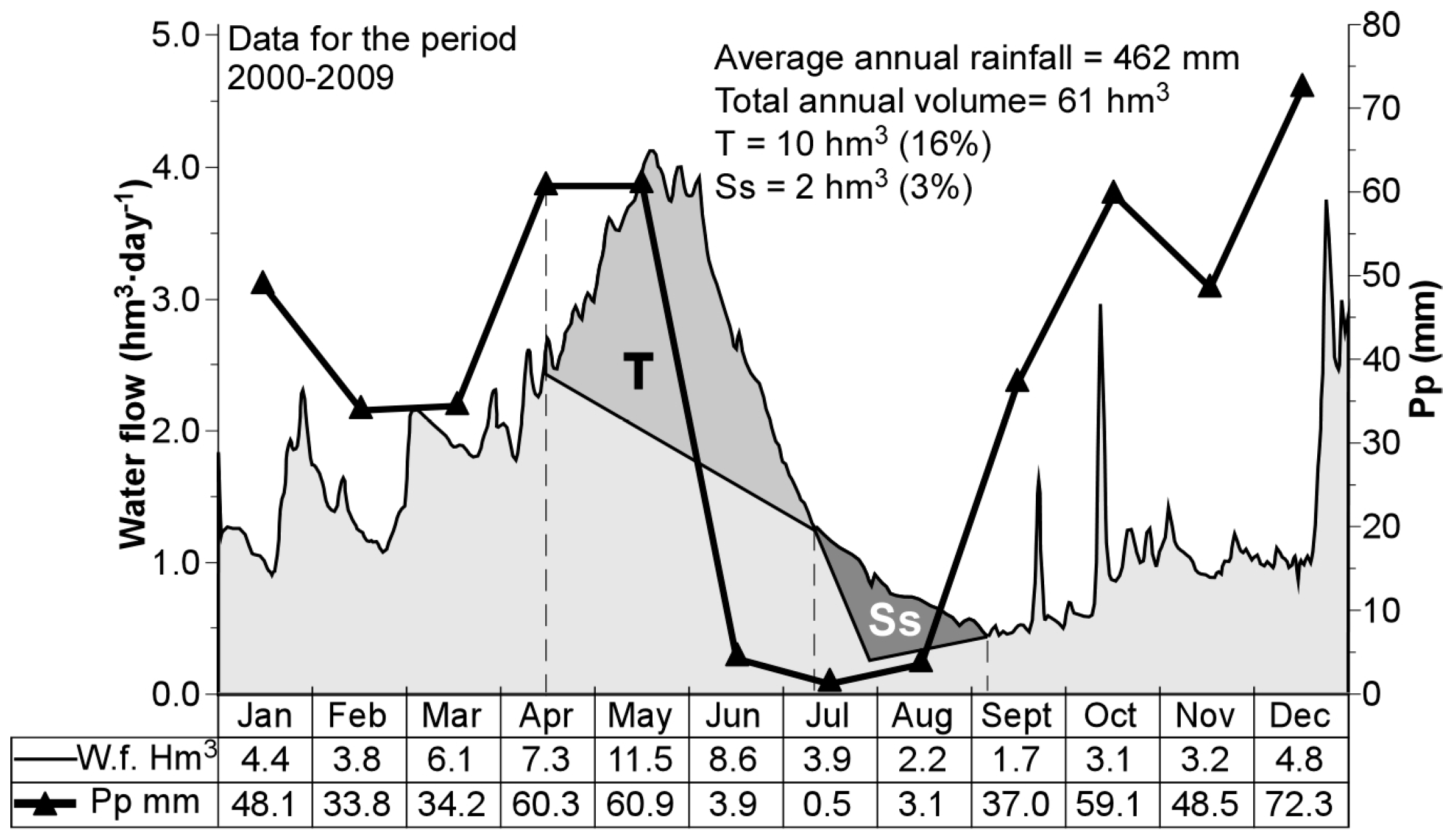
The estimation of different components of water volumes discharged during the main period of thaw is based on
Figure 8 (built with data of
Figure 7b). We therefore specify that due to the addition of snowmelt to mean precipitation in March-April the water-flow increases. Precipitation increased in April and May to around 60 mm each month, while the water-flow continues its increasing trend. At this point the thaw increases surface water-flow (intersection of the dotted line and the water-flow curve). Water-flow reaches its maximum in mid-May (4.1 hm
3·day
−1) due to the prevalence of sub-surface supplies under these conditions (1.2 hm
3·day
−1). Another change occurs in the water-flow slope (first half of September, minimum at 0.5 hm
3·day
−1) due to fresh rainfall supply. In summary, the total mean water volume draining to the head of the Genil River for the period 2000–2009 is 61 hm
3 (
Figure 8, sum of the mean monthly values); the water drained during the main thaw is T = 10 hm
3 (16%), and the water contributed by sub-surface resources is Ss = 2 hm
3 (3%), values obtained by planimetry of each area.
Finally, we should point out that in the months of the second half of autumn and first half of winter (mainly October to December) there is a noticeable lag between precipitation and water-flow increase, as precipitation mainly takes the form of snow that lies on the peaks for months.
The comparison of these results with those obtained by the national program “Evaluation of Water Reserves Resulting from Snowfall” [
36], shows that 14 hm
3 of water accumulate as snow at the head of the Genil River. The orders of value are similar, but several reasons can be found for the differences: (i) The periods considered in each analysis can have different precipitation; (ii) thaw volumes can be attributed to a different period of the year (whole year or only pre-summer), and (iii) different methodologies used. In any case, our calculations refer to the high western peaks of the massif, where there are numerous heavily sloping areas, with a consequently thinner layer of snow [
37].
3.3. Water-Bodies and Green Fringes
Together with the water-bodies, we often find high mountain green fringes, locally called “borreguiles”. The total surface area of these associated green fringes is approximately 186,500 m2, for a total number of 84, of which 58 are found on the Mediterranean watershed (149,000 m2) and 26 on the Atlantic (37,000 m2). These green fringes also reflect the moistening-drying cycles undergone by the adjoining water-bodies.
3.3.1. Types of Water-Bodies in Relation to Green Fringes
From the viewpoint of the interrelation between green fringes and water-bodies, we can distinguish three types of water-bodies:
• Water-bodies without green fringes
The total number of water-bodies without green fringes is 39 (32% of the overall total), 14 on the Mediterranean watershed (all above 2880 m a.s.l.) and 25 on the Atlantic (18 above 2880 m a.s.l.). It should be noted that out of the total of six large-scale water-bodies with over 5000 m3 water volume, three do not have green fringes. These are Vacares, Caldera and Altera (Mediterranean watershed), the first two normally survive the summer drought.
• Water-bodies with small green fringes
These water-bodies have green fringes of less than 1000 m2. They are restricted to small, gently sloping steps around the water’s edge, which are suitable for narrow bands of vegetation. This is the case of Laguna Larga (Atlantic watershed), Laguna del Caballo and Laguna Cuadrada (Mediterranean watershed). In all, there are 45 cases (36% of the total), 12 on the Atlantic watershed (two above 2880 m a.s.l.) and 33 on the Mediterranean (25 above 2880 m a.s.l.).
• Water-bodies with extensive green fringes
These include green fringes extending to over 1000 m
2 and almost entirely surrounding the water-bodies. There is interconnection between the water sheet and surrounding vegetation in both time (for several weeks at least) and space over gently sloping surfaces which accumulate fine detrital material, with ideal field capacity. This allows for conservation of part of the vegetation as the summer drought advances, and the abundant root system guarantees continuity of the vegetation in successive years. The best examples are Laguna Hondera (
Figure 2e, Mediterranean watershed) and part of the Lagunillos de la Virgen (Atlantic watershed). We counted 39 cases (32%), 14 on the Atlantic watershed (six above 2880 m a.s.l.) and 25 on the Mediterranean (16 above 2880 m a.s.l.).
3.3.2. Distribution of Green Fringes and Water-Bodies by Altitude
Throughout the massif (
Figure 6d) the highest number of green fringes occurs in the 2900–3000 m a.s.l. interval (37%) with Gaussian distribution. Approximately 60% of them are located between 2800 and 3000 m a.s.l. However, green fringe surface area is highest at 2800–2900 m a.s.l. (36%), although 63% of this surface is concentrated in the 2800–3000 m a.s.l. range. The surface area of the water sheet of these bodies is irregularly distributed, with 50% of all the water-bodies located equally between the 2800–2900 and 2900–3000 m a.s.l. intervals. There is a noticeably high percentage (29%) of water sheet area in the 3000–3100 m a.s.l. interval. These values agree with the number of water-bodies observed (
Figure 6a).
The distribution of green fringes in the entire massif (
Figure 6d) is largely determined by their characteristics on the Mediterranean watershed (
Figure 6e), which also agree with our comments on the water-bodies in
Section 3.1.3.2. On the Mediterranean watershed, 43% of the green fringes are found in the 2900–3000 m a.s.l. interval, and 65%, representing 62% of the green fringes area on this watershed, are found between 2800 and 3000 m a.s.l. The water sheet of the water-bodies in the 3000–3100 m a.s.l. interval represents 41% of the area occupied by water on this watershed.
The Atlantic watershed (
Figure 6f) has an irregular distribution in this regard, where the green fringes and water-bodies become less important above 3000 m a.s.l. The green fringes between 2800 and 2900 m a.s.l. represent 38% of the total, with 35% below 2700 m a.s.l. The surface occupied by green fringes in the 2800–2900 m a.s.l. interval represents 46%. The surface area of the water sheet has maximum values in the 2700–2800 m a.s.l. interval (43%).
4. Discussion
It has always been a challenge to determine the number of water-bodies in mountainous areas. Apart from the inherent difficulties of the terrain, the most important difficulty lies in correctly defining the concept of water-body, which must avoid being rigid, in order to better adapt to the diverse circumstances found on this massif. In our case, in a context of high ecological value coexisting with extreme annual and year-on-year climatic variations, any naturally collected water-body has been considered relevant.
4.1. Uneven Distribution of Water-Bodies
The persistence of snow is a necessary condition for the presence of the water-bodies studied here, but it alone is not sufficient, as suitable basins are required for the accumulation of water, and their position in the landscape must encourage permanence.
The southern orientation of the Mediterranean watershed offers a priori less favorable conditions for the creation of water-bodies than the northern or Atlantic watershed. It is reasonable to suppose that in the northern hemisphere snow would last longer on northern facing mountain slopes due to lower insolation, and for this reason we might expect a higher number of water-bodies on this watershed of Sierra Nevada. Surprisingly, however, we have found the opposite (
Figure 5). The Mediterranean watershed (
Figure 5(a2)) contains 72 water-bodies (58%), whereas the Atlantic basin (
Figure 5(a3)) has only 51 (41%). Equally, if we set 2700 m a.s.l. as the altitude above which snow is more stable and is therefore more suitable for the concentration of water-bodies (111 water-bodies), we find that the number of water-bodies in the Mediterranean basin is even higher than that of the Atlantic basin (70 vs. 41,
Figure 5). We also reach a similar conclusion for the number of specimens at altitudes above 2840 m a.s.l. (59 vs. 34,
Figure 5). However, the opposite is found in the distribution at altitudes below 2700 m a.s.l. (two vs. 10 water-bodies), although in this case the number of water-bodies is low.
A plausible explanation for this fact has been found in cross-sections performed in two representative valleys (Guarnón, on the northern watershed of Sierra Nevada, and Mulhacén River, on the southern,
Figure 9). The overall slope of the Mediterranean watershed is around 20% (~11°) as against the 31% (~17°) of the Atlantic watershed. The detail is much more significant. After a common steep area caused by the great peaks (categories I and α, with slopes >70% (~35°), the Mediterranean area has an open sigmoidal cross-section, with a large convex area (category II, around 2 km long, close to the steep area), and a slope around 18% (~10°), where the maximum numbers of water-bodies (63) are concentrated, but there is no equivalent on the Atlantic watershed. This is where highest specific surface areas are found (
Table 2), suggesting rougher terrain, more suitable to host water-bodies. In summary, although at high altitude there is limited space to house water-bodies, the Mediterranean water-bodies fit better at these heights than those of the Atlantic watershed because of its slope. This agrees with
Figure 5 and
Figure 6a–c.
However, we do not know whether this means that glacier niches developed more easily on one watershed than the other. Indeed, the Mediterranean watershed has 10 headwaters, while the Atlantic has 7 headwaters (
Table 2). But the fact that the Mediterranean watershed suffers more freeze-thaw cycles every year must cause higher alteration of its lithological substratum than in the Atlantic watershed and, consequently, the amount and quality of debris should be different. Both features can be linked to the type of moraines associated with the water-bodies. The Mediterranean watershed has four moraines, at the water-bodies of Caballo, Caldera and Vacares (formed by heterometric debris about 50% of which consists of the <2 mm fraction), and Altera (with very scarce or no fine fraction,
Figure 2f). On the other hand, the Atlantic watershed has two moraines, at the water-bodies of Corral del Veleta and Valdeinfierno. These features should also be extensible to the soil textures, although soil depths have to be considered in the framework of an altered material, beyond the limit of biological activity. Therefore, we have two watersheds with different orientation, which determines different degrees of lithological alteration as a differential factor for the development of the hillside morphologies holding the studied water-bodies.
The distribution of the volumes of the water-bodies studied (
Figure 6d–f) allows us to ask questions about the prevalence of small-size water-bodies and whether climate change is the cause. Several circumstances coincide on these points, although at the actual state of knowledge there is a considerable amount of speculation. First of all, the geomorphology of the high peaks of Sierra Nevada provides very restricted spaces to house larger water-bodies. Optionally, some water-bodies could decrease in size due to silting, as might be the case of the water-bodies at present surrounded by extensive green fringes (e.g., Laguna Hondera,
Figure 2e). However, these are few and found in exceptional settings.
4.2. Hydrology and Thaw
The dependence and relation of the water-bodies to altitude (
Figure 5a) can be explained by the mainly solid nature of the precipitation and by the presence of basins in suitable places. After the snow cover is established, temperature acts as the main regulator of the snowmelt flow. Surface hydrological processes of a general nature then begin and their gradual thawing at these latitudes facilitates the survival of the water-bodies during part or all of the summer. The thaw mainly takes place in the passage from spring to summer (pre-summer melt) lasting one to three months, depending on the amount of snow accumulated in the year (
Figure 7b), and determines the various stages of plant growth.
The water-flows obtained for the headwaters of the Genil River for the period of study (
Figure 8) establish that the mean volume of pre-summer snowmelt in this basin is 10 hm
3 and sub-surface flow is 2 hm
3. These flows mainly occur as a result of snow melting above 2500 m a.s.l., which is more stable than the snow accumulated at lower levels. We thus obtain a coefficient of sub-surface and melt water supply of 0.062 and 0.309 hm
3·km
−2 respectively, which allows us to estimate the water volumes on the Mediterranean watershed and, thereby, for the sector of massif studied (
Table 3).
In consequence, the western sector of Sierra Nevada (considering altitudes above 2500 m a.s.l. on both watersheds) supplies a mean of approximately 53 hm
3 by pre-summer snowmelt for the period studied (
Figure 8,
Table 3). The sub-surface supply is small, estimated at an average of 11 hm
3 for the sector studied, of which 8 hm
3 correspond to the Mediterranean watershed. In other words, as expected, the relative percentage of water contained in the water-bodies is small, as it is no more than 0.5% of the snowmelt, and less than 2.4% of the sub-surface water.
The application of the hydrological behaviour of the Atlantic watershed of Sierra Nevada to the Mediterranean watershed should assume the aforementioned “asymmetry” of insolation on one watershed and the other. Therefore, the main effect that could be forecast is that the Mediterranean watershed would have an earlier main annual thawing period and its summer drought would be longer. In other words, the vegetation period would be longer, but so too would the period of water deficit.
4.3. Water-Bodies and Green Fringes
Although the total water volume retained in the water-bodies of Sierra Nevada is small,
Table 4 allow us to determine some additional relations between water-bodies and their associated green fringes, as they together give an indication of the natural water-efficiency in terms of the surface area of this type of biotopes. We consider these relations to be a consequence of the geomorphological aspects and solar exposure commented above.
We observe that, in the massif as a whole (
Table 4), there were 84 water-bodies with green fringes (68%). When classified by volume, we found only six water-bodies >5000 m
3, of which three had green fringes, totaling 7426 m
2. The 117 remaining water-bodies of the massif were all <5000 m
3, of which 81 had green fringes totaling 179,044 m
2 and representing 96% of the surface area occupied by green fringes associated to water-bodies in this sector of the massif. This shows “passive” behaviour of the larger water-bodies, acting as mere pools of still water with little influence on the development of green fringes. Several reasons explain this apparently “passive” behaviour. The variations in water level prevent the establishment of a plant layer, because each rise or fall of the water level causes a subaquatic regime or permanent drought, with hardly any intermediate stages, given the strongly sloping sides. Moreover, on the edges of such pools there is practically no soil surface with water supply to maintain a suitable degree of humidity. Water-bodies such as Vacares and Caldera are examples of this. Finally, if the water-body is surrounded by chaotic loose rocks, rapid percolation will predominate and the absence of a suitable substratum prevents vegetation rooting to create green fringes. This is the case of Laguna Altera (
Figure 2f) and the largest water-body in the Corral del Veleta.
Table 4 also shows different behaviours between the Atlantic and Mediterranean watersheds. Apart from the different number of water-bodies in both basins, the number and development of the associated green fringes have clear differences: 26 of the water-bodies on the Atlantic watershed (50% of this watershed) have green fringes, as against 58 of those on the Mediterranean (80%). The surface area occupied by these green fringes on the Mediterranean watershed represents 80% of the green fringes on the entire massif. The total water volume and the green fringe surface area on the Mediterranean watershed are 1.9 and 3.9 times those of the Atlantic watershed. Stratification of the water-bodies by size shows that on the Atlantic watershed there are only two larger than 5000 m
3 with a total volume of 56,388 m
3 and both have green fringes (6797 m
2), whereas the Mediterranean has four water-bodies containing 78,288 m
3 of water, but there is only one green fringe 629 m
2 in size. If we consider the <5000 m
3 water-bodies, we find 49 on the Atlantic watershed (42% of those in this range) containing 18,343 m
3 of water and whose associated green fringes occupy 30,885 m
2 (17%). The Mediterranean watershed has 68 water-bodies (58%) containing 62,053 m
3 of water, and associated green fringes occupying 148,159 m
2, i.e., 83% of the surface area occupied by green fringes in this range, which is 4.8 times higher than those of the Atlantic watershed. We also see in this table that, within a single size range, the large water-bodies (>5000 m
3) are too few in number to obtain reliable deductions, although their “passivity” in comparison with the smaller water-bodies is clear. For the latter (<5000 m
3), the water volumes on the Mediterranean watershed are 3.5 times larger than those of the Atlantic watershed.
If efficiency is achieving more with less, we can define water-efficiency as the quotient between green fringe surface area and the water volume in the associated water-bodies. So, the efficiency in Sierra Nevada is 40 times higher in the smaller water-bodies than in the large ones. Regarding the Atlantic and Mediterranean watersheds, this efficiency is respectively 13.9 and 297.1 times higher in the smaller water-bodies than in the large ones (
Table 4), that is, the green fringes of the smaller water-bodies of the Mediterranean side are 21.3 times more efficient than those of larger ones on the Atlantic side.
However, glacial modelling does not seem to be the main cause of these differences, as the number of snowfield niches seems to be approximately similar. Glacial modelling itself shows differences in the same sense, as the number of niches and moraines on each watershed have small, but detectable differences.
5. Conclusions
Although many parts of the Mediterranean mountains lack reliable, long-term records of river flows, we have estimated that in this massif pre-summer thawing produces 53 hm3 of run-off and 11 hm3 of subsurface flow. The annual timing of this thaw mainly occurs in May–June, as a function of the particular climatology of each year; the sub-surface contribution mainly occurs in July–August.
The water volume stored in all the water-bodies of the western sector of Sierra Nevada is small, with less than 0.25 hm3 in all 123 inventoried water-bodies. This water volume represents 0.9/2.4% of thaw/sub-surface volumes, respectively. Most of this water is contained in a few water-bodies: 60% of it is found in the three largest water-bodies.
The water in the water-bodies is unevenly distributed between the Atlantic and Mediterranean watersheds. At these latitudes the northern watershed should have a lower water deficit than the southern as it receives less insolation, and one might expect it to have more water-bodies or, at least, to store a larger volume of water. However, we observe exactly the opposite: the Atlantic watershed has 51 water-bodies (40%) as against 72 on the Mediterranean watershed (60%), and the volume stored on the Atlantic side is 75,000 m3 (35%) as against 140,000 m3 (65%) on the Mediterranean.
The distribution of water-bodies is also uneven by altitude. The general characteristics of the massif by altitude ranges are to a large extent defined by the characteristics of the water-bodies on the Mediterranean watershed. This watershed has more development in number and volume of these water-bodies between 2900 and 3100 m a.s.l.
The green fringes associated to the water-bodies underline even more the differences between the two watersheds, with 26 green fringes (31%) on the Atlantic one, with a total surface area of 38,000 m2 (20%), as against 58 green fringes on the Mediterranean one (69%) totaling 149,000 m2 (80%). Apart from the lower gradient of the slope, the apparent imbalance observed between the number of water-bodies and the surface area of associated green fringes can be explained by the fact that the higher insolation of the Mediterranean watershed increases the growing period, and so the water-efficiency is optimized, despite the increase in water deficit.
The area of the green fringes associated with the three largest water-bodies is very small, totaling 7426 m2 (0.04% of the total). On the contrary, the <5000 m3 water-bodies on the Mediterranean watershed have a surface area 4.8 times larger than those on the Atlantic watershed. On the same watershed, the water-efficiency of the Atlantic green fringes associated with small water-bodies is 13.9 times than those associated with large bodies, and on the Mediterranean watershed, the efficiency of the green fringes associated with small water-bodies is two orders of magnitude higher than in the large ones.
This hydric “asymmetry” can largely be justified by geomorphological arguments, such as the difference in gradient of the slopes, causing different solar orientation and exposure which thereby affect its ecological functions.
There is, therefore, a lack of studies in other similar regions of the world, especially those related with Mediterranean mountains, concerning the paradoxes detected in this study, such as the relations between water and green fringes, and the hydric asymmetry detected here.
Author Contributions
Both authors have contributed to the conceptualization, methodology, formal analysis, investigation, resources, writing—original draft preparation and writing—review and editing.
Funding
This research received no external funding
Acknowledgments
We wish to thank our colleagues A. Sánchez Salvador (Consejería de Medio Ambiente, Junta de Andalucía), and P. Martínez Santos (Universidad Complutense, Madrid), who have provided insight and expertise that greatly assisted the research. We would also like to show our gratitude to Google Earth, Google Maps and Iberpix technologies which have made it easier to find the exact location of all points studied and have facilitated carrying out the cartography, as well as to the Ministry of Agriculture, Fisheries, Food and Environment (MAPAMA) for its valuable support in providing the hydrological data.
Conflicts of Interest
The authors declare no conflict of interest.
References
- UNESCO, Biosfere Reserve. 2017. Available online: http://www.unesco.org/new/en/natural-sciences/environment/ecological-sciences/biosphere-reserves/eureur-north-america/spain/sierra-nevada/ (accessed on 8 May 2018).
- Heywood, V.H. The Mediterranean flora in the context of world diversity. Ecol. Mediterr. 1995, 21, 11–18. [Google Scholar]
- Médail, F.; Quézel, P. Biodiversity hotspots in the Mediterranean basin: Setting global conservation priorities. Conserv. Biol. 1999, 13, 1510–1513. [Google Scholar] [CrossRef]
- Myers, N.; Mittermeier, R.A.; Mittermeier, C.G.; da Fonseca, G.A.B.; Kent, J. Biodiversity hotspots for conservation priorities. Nature 2000, 403, 853–858. [Google Scholar] [CrossRef] [PubMed]
- Alvarez-Cobelas, M.; Rojo, C.; Angeler, D.G. Mediterranean limnology: Current status, gaps and the future. J. Limnol. 2005, 64, 13–29. [Google Scholar] [CrossRef]
- Bolle, H.J. Mediterranean Climate: Variability and Trends; Springer: Berlin, Germany, 2003. [Google Scholar]
- Woodward, J.C. Introduction. In The Physical Geography of the Mediterranean; Woodward, J.C., Ed.; Oxford University Press: Oxford, England, 2009; pp. 3–4. [Google Scholar]
- McNeill, J.R. The Mountains of the Mediterranean World; Cambridge University Press: Cambridge, UK, 1992. [Google Scholar]
- Price, M.F. Mediterranean Mountain Environments. Mt. Res. Dev. 2013, 33, 355–356. [Google Scholar] [CrossRef]
- Vogiatzakis, I. Mediterranean Mountain Environments; Wiley: Hoboken, NJ, USA, 2012. [Google Scholar]
- Thornes, J.B.; López-Bermúdez, F.; Woodward, J.C. Hydrology, river regimes, and sediment yield. In The Physical Geography of the Mediterranean; Woodward, J.C., Ed.; Oxford University Press: Oxford, England, 2009; pp. 229–253. [Google Scholar]
- IGME. Mapa geológico de España a escala 1:50.000, N° 1042 (Lanjarón); Serie MAGNA; Instituto Geológico y Minero de España: Madrid, Spanish, 1979. [Google Scholar]
- IGME. Mapa geológico de España a escala 1:50.000, N° 1027 (Güéjar Sierra); Serie MAGNA; Instituto Geológico y Minero de España: Madrid, Spanish, 1980. [Google Scholar]
- IGME. Mapa geológico de España a escala 1:50.000, N° 1028 (Aldeire); Serie MAGNA; Instituto Geológico y Minero de España: Madrid, Spanish, 1981. [Google Scholar]
- Puga, E.; Díaz de Federico, A.; Nieto, J.M. Tectonostratigraphic subdivision and petrological characterisation of the deepest complexes of the Betic zone: A review. Geodin. Acta 2002, 15, 23–43. [Google Scholar] [CrossRef]
- Gómez-Ortiz, A.; Sánchez-Gómez, S.T.; Simón-Torres, M. Geomorphological Map of Sierra Nevada. Glacial and Periglacial Geomorphology; Junta de Andalucía-Universidad de Barcelona: Barcelona, Spanish, 2002. [Google Scholar]
- Schulte, L. Climatic and human influence on river systems and glacier fluctuations in southeast Spain since the Last Glacial Maximum. Quat. Int. 2002, 93–94, 85–100. [Google Scholar] [CrossRef]
- Hughes, P.D.; Woodward, J.C. Timing of glaciation in the Mediterranean mountains during the last cold stage. J. Quat. Sci. 2008, 23, 575–588. [Google Scholar] [CrossRef]
- Gómez Ortiz, A.; Schulte, L.; Salvador-Franch, F.; Palacios-Estremera, D.; Sanjosé Blasco, J.J.; Atkinson Gordo, A. Deglaciación reciente de Sierra Nevada. Repercusiones morfogénicas, nuevos datos y perspectivas de estudio futuro. Cuadernos de Investigación Geográfica 2004, 30, 147–168. [Google Scholar] [CrossRef]
- Anderson, R.S.; Jiménez-Moreno, G.; Carrión, J.S.; Pérez-Martínez, C. Postglacial history of alpine vegetation, fire, and climate from Laguna de Río Seco, Sierra Nevada, Southern Spain. Quat. Sci. Rev. 2011, 30, 1615–1629. [Google Scholar] [CrossRef]
- Jiménez-Moreno, G.; Anderson, R.S. Holocene vegetation and climate change recorded in alpine bog sediments from the Borreguiles de la Virgen, Sierra Nevada, southern Spain. Quat. Res. 2012, 77, 44–53. [Google Scholar] [CrossRef]
- MAPAMA, Ministry of Agriculture and Fisheries, Food and Environment. SAIH Sistema de Información. 2017. Available online: http://www.mapama.gob.es/es/agua/temas/evaluacion-de-los-recursos-hídricos/SAIH/default.aspx (accessed on 31 January 2018).
- Oliva, M. Quaternary landscape evolution of Sierra Nevada (Southern Spain): State of the art. Rev. Cuater. Geomor. 2011, 25, 21–44. [Google Scholar]
- Google Earth Digital GlobeImagery. Available online: https//:www.google.es/intl/es/earth/index.html (accessed on 19 December 2017).
- Quézel, P. Definition of the Mediterranean region and the origin of its flora. In Plant Conservation in the Mediterranean Area; Gómez-Campo, C., Ed.; Springer: Dordrecht, The Netherlands, 1985. [Google Scholar]
- Blondel, J.; Aronson, J. Biology and wildlife of the Mediterranean region. J. Nat. Hist. 1999, 38, 1723–1724. [Google Scholar] [CrossRef]
- Rivas-Martínez, S. Mapa de series, geoseries y geopermaseries de vegetación de España. Memoria del mapa de vegetación potencial de España, Parte I. Itinera Geobot. 2007, 17, 5–436. [Google Scholar]
- Fernández-Calzado, M.R.; Molero-Mesa, J. Changes in the summit flora of a Mediterranean mountain (Sierra Nevada, Spain) as a possible effect of climate change. Lazaroa 2013, 34, 65–75. [Google Scholar] [CrossRef]
- Fernández-Calzado, M.R.; Molero-Mesa, J. The cartography of vegetation in the cryoromediterranean belt of Sierra Nevada: A tool for biodiversity conservation. Lazaroa 2011, 32, 101–115. [Google Scholar]
- IGN. Mapa Topográfico Nacional a escala 1:25.000, N° 1027 and 1028; Instituto Geográfico Nacional: Madrid, Spanish, 2000.
- Iberpix. Available online: https://www.ign.es/iberpix2/visor/ (accessed on 19 December 2017).
- Alford, D. Spatial patterns of snow accumulation in the Alpine terrain. J. Glaciol. 1980, 26, 517. [Google Scholar] [CrossRef][Green Version]
- Alford, D. The orientation gradient: Regional variations of accumulation and ablation in alpine basins. In Geoecology of the Colorado Front Range: A Study of Alpine and Subalpine Environments; Ives, J.D., Ed.; West View Press: Boulder, CO, USA, 1980; pp. 214–223. [Google Scholar]
- Elder, K.; Dozier, J.; Michaelsen, J. Spatial and temporal variation of net snow accumulation in a small alpine watershed, Emerald lake basin, Sierra Nevada, California, USA. Ann. Glaciol. 1989, 13, 56–63. [Google Scholar] [CrossRef]
- Birkeland, K.W. Terminology and predominant processes associated with the formation of weak layers of near-surface faceted crystals in the mountain snowpack. Arct. Alp. Res. 1998, 30, 193–199. [Google Scholar] [CrossRef]
- MAPAMA, Ministry of Agriculture and Fisheries, Food and Environment. ERHIN Programme (Evaluation of the Hydric Resources Coming from Innivation). 2013. Available online: http://www.mapama.gob.es/es/agua/temas/evaluacion-de-los-recursos-hídricos/ERHIN/default.aspx (accessed on 31 January 2018).
- Wirz, V.; Schirmer, M.; Gruber, S.; Lehning, M. Spatio-temporal measurements and analysis of snow depth in a rock face. Cryosphere 2011, 5, 893–905. [Google Scholar] [CrossRef]
Figure 1.
(a) Location of Sierra Nevada in the framework of the southeast Iberian Peninsula, and limits of the National and Natural Parks. The triangle indicates the position of the Mulhacén peak (3479 m a.s.l.). (b) Main catchments.
Figure 1.
(a) Location of Sierra Nevada in the framework of the southeast Iberian Peninsula, and limits of the National and Natural Parks. The triangle indicates the position of the Mulhacén peak (3479 m a.s.l.). (b) Main catchments.
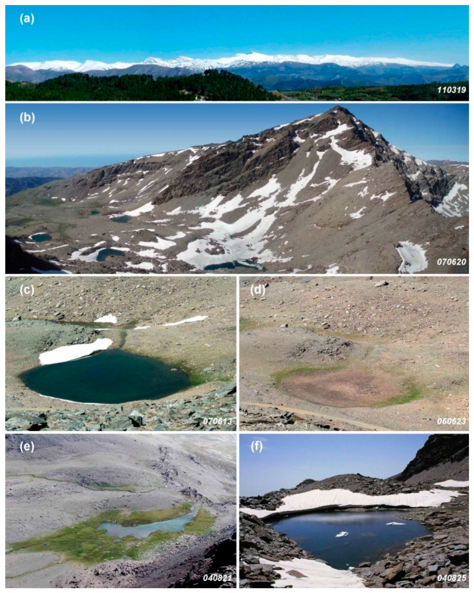
Figure 2.
Water-bodies in Sierra Nevada. (a) General view of Sierra Nevada at the end of winter, mostly corresponding to the Atlantic watershed. The highest peaks appear at the centre–centre left of the image. (b) General view of the Siete Lagunas valley (Mediterranean watershed), sprinkled with water-bodies, taken from La Alcazaba peak, opposite the Mulhacén peak. Note the snow recession. (c,d) Caldereta with and without water. Observe the presence of a green fringe strip (328 m2). Dimensions: 58.0 × 47.0 × 1.65 m; height: 3039 m a.s.l. (e) Laguna Hondera, surrounded by the largest fringe of vegetation (34,000 m2). Dimensions: 162 × 59 × 0.65 m; height: 2898 m a.s.l. (f) Altera, the highest of Siete Lagunas valley (included in image (b)) with snow late in the thaw period, and no green fringes; the relief of the bottom corresponds to a very rocky, permeable moraine. Dimensions: 93.6 × 79.0 × 3.80 m; height: 3066 m a.s.l. Numbers in lower right corner indicate the date of each photograph (year, month, day).

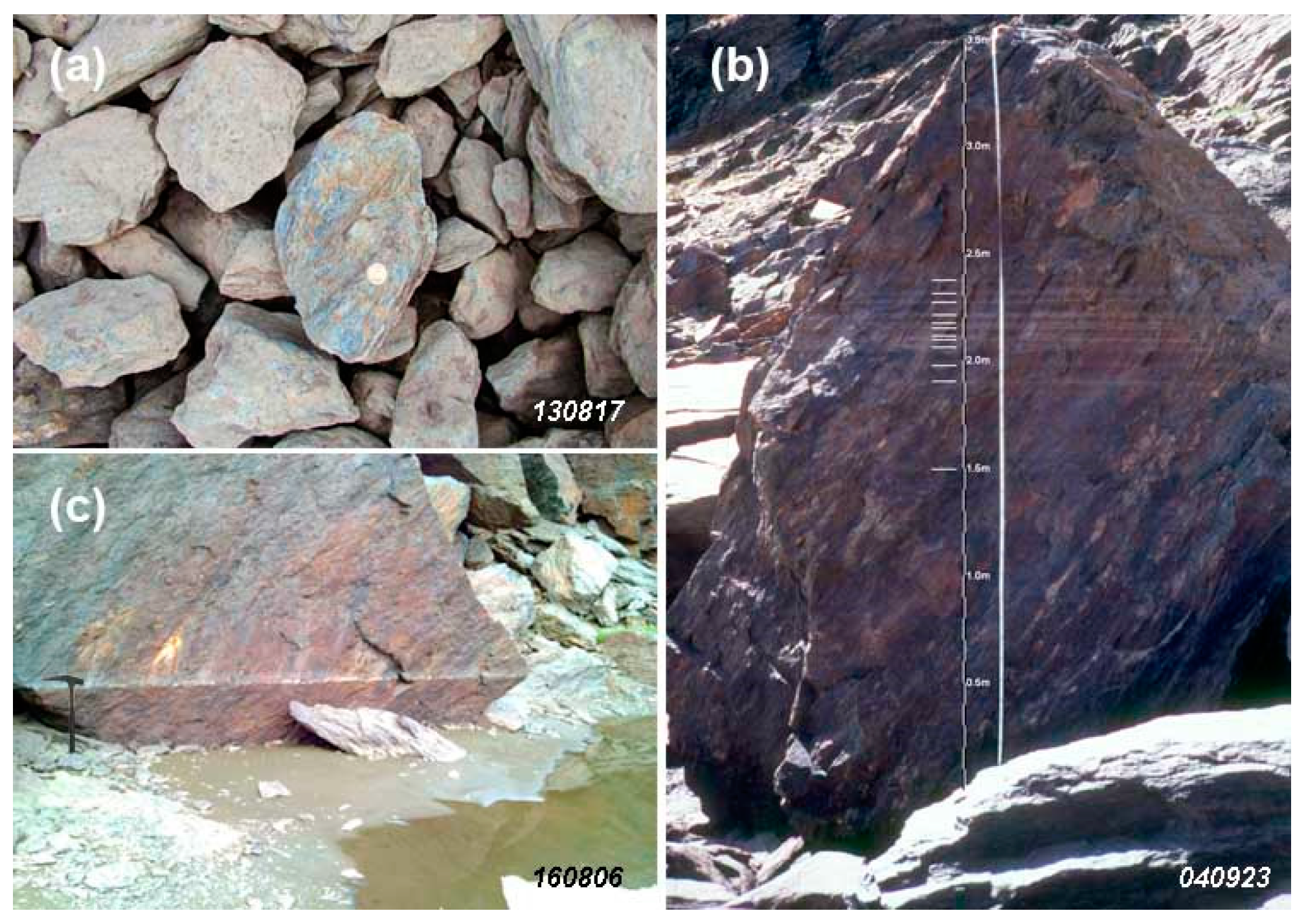
Figure 3.
Some features to determine the presence of water-bodies and their depth. (a) Rocky bottom coated with a fine film of sediment. By contrast, the coin is on an uncoated stone. (b) “Palaeo-levels” preserved in a block on the edge of Laguna de Vacares (height: 2880 m a.s.l.). Numbers of the bar near the measuring tape show depths every half meter. Lines between 1.5 and 2.5 m indicate the “palaeo-levels” identified. (c) Similar to the previous in an unnamed pond found in the Lanjarón river catchment (height: 2953 m a.s.l.). In this case we have only observed one “paleo-level” clearly marked. Numbers in lower right corner indicate the date of each photograph (year, month, day).
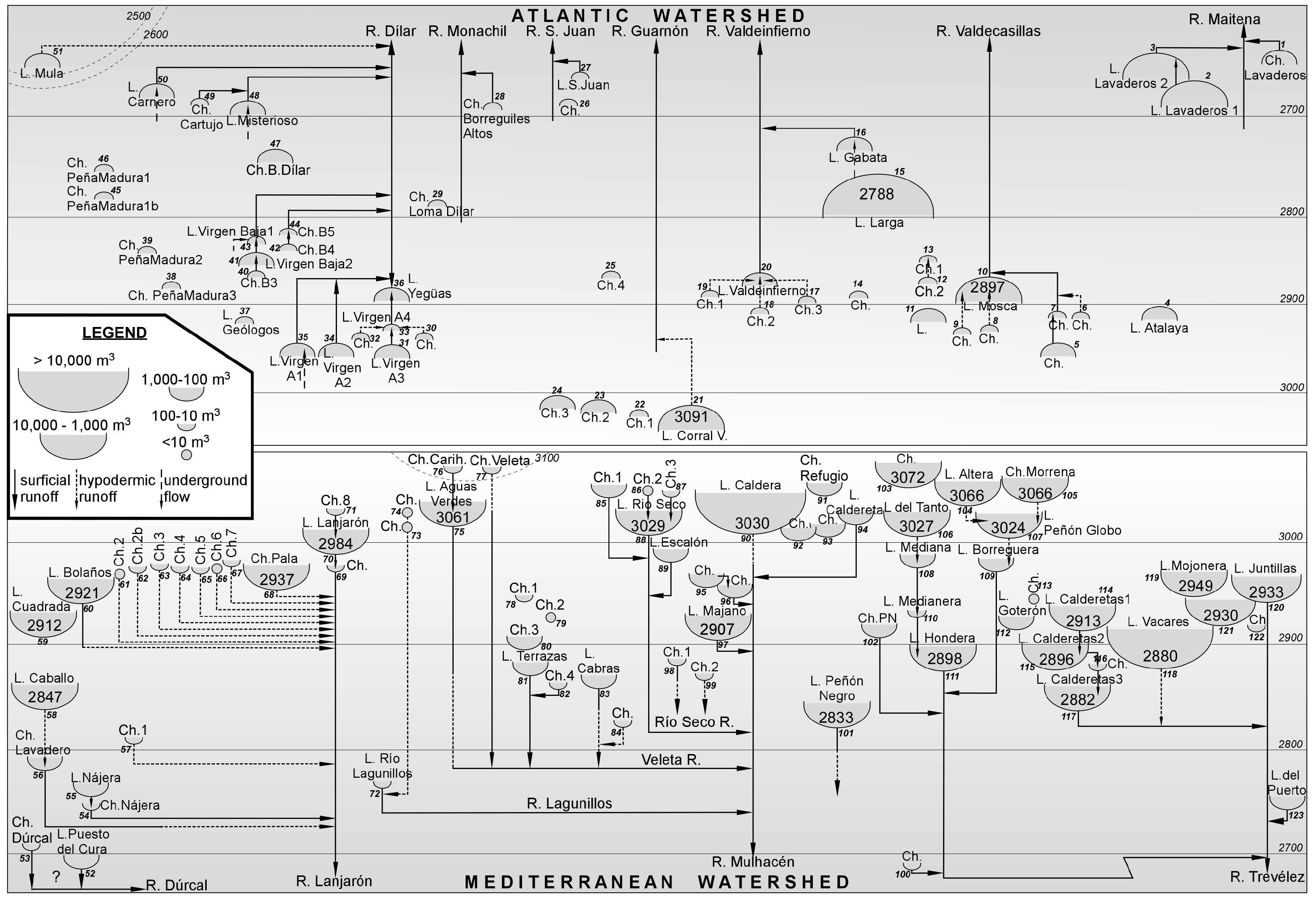
Figure 4.
Sketch showing the positional relationships between the water-bodies of the Sierra Nevada massif, ordered by watersheds and headwaters. Heights (m a.s.l.) of main water-bodies are specified (numbers included in the larger bodies), as well as classification by volume (Legend). Also shown are potential underground flows in the water-bodies (springs) and infiltrations occurring in the effluents. The lowest water-bodies, such as Laguna Seca and Loma de las Cunas (<2500 m a.s.l.) are not included. Small numbers near each water-body indicate the order number.
Figure 5.
(a) Histogram showing the number of water-bodies distribution (N) by height (m a.s.l.) at 40 m intervals: (a1) throughout the entire Sierra Nevada. (a2) Idem on the Mediterranean watershed. (a3) Idem on the Atlantic watershed. Nt = total number of water-bodies. (b) Histogram showing the skewed distribution of water volumes (m3) at intervals of 200 m3: (b1) throughout the Sierra Nevada massif. (b2) Idem on the Mediterranean watershed. (b3) Idem on the Atlantic watershed. Nt = total number of water-bodies.
Figure 6.
Upper file: relationships between water-bodies and water volumes between 2700 and 3200 m a.s.l. (at 100 m intervals) regarding: (a) total massif; (b) Mediterranean watershed; (c) Atlantic watershed. Abbreviations: %Wb = percentage of water-bodies; %Wv = percentage of water volumes. Lower file: relationships between green fringes (both the number of cases and their surfaces) and associated water-bodies between 2700 and 3200 m a.s.l. (100 m intervals) regarding: (d) total massif; (e) Mediterranean watershed; (f) Atlantic watershed. Abbreviations: %Gf = percentage of number of green fringes; %GfS = percentage of green fringes (surface area); %WsS = percentage of water-sheet (surface area).
Figure 7.
(a) Monthly evolution of rainfall (bars) and water-flow (continuous line) during the period 1999–2017 for the Canales hydrological station (Genil River, Atlantic watershed). Annual precipitations are indicated by the numbers between dashed lines. (b) Hydrograms for the Canales hydrological station (1999–2009) obtained from hourly data. Arrows highlight the moment of maximum snowmelt discharge. Numbers on left indicate precipitation (Pp) in the hydrological year.
Figure 8.
Mean hydrogram for 2000–2009 for the head of the Genil River showing daily water-flow (fine line) re-calculated as hm3 in each month (underlying table), and precipitation (thick line with filled triangles). T = Thaw contribution; Ss = Sub-surface contribution.
Figure 8.
Mean hydrogram for 2000–2009 for the head of the Genil River showing daily water-flow (fine line) re-calculated as hm3 in each month (underlying table), and precipitation (thick line with filled triangles). T = Thaw contribution; Ss = Sub-surface contribution.
Figure 9.
Geomorphological cross-section of two representative valleys of Sierra Nevada: Mulhacén River (Mediterranean watershed; slope stretches indicated by Roman numbers) and Guarnón River (Atlantic watershed; slope stretches indicated by Greek letters). The number (N) of water-bodies in each stretch is also indicated. Numbers in brackets (adjoining tables) indicate: for the global slope, the quotient between altitude/length; for other areas, range of altitudes in which the slope is defined. Vertical scale = Horizontal scale.
Table 1.
Climatic data from three meteorological stations in the study area, for the period 2000–2017.
Table 1.
Climatic data from three meteorological stations in the study area, for the period 2000–2017.
| Station | Altitude (m) | Watershed | Pp Mean (mm) |
|---|
| Canales [22] | 959 | Atlantic | 540 |
| Univ. Hostel [23] | 2507 | Atlantic | 710 |
| Capileira [22] | 1588 | Mediterranean | 507 |
Table 2.
General features of the headwaters of western Sierra Nevada containing water-bodies *.
Table 2.
General features of the headwaters of western Sierra Nevada containing water-bodies *.
| | Headwater | Height (m a.s.l.) | Surface | Perimeter | Water-Bodies | Water | Green Fringes |
|---|
| | Max | Min | S (km2) | P (km) | Ner. | V (m3) | S m2 |
|---|
| Atlantic watershed | Dílar | 3396 | 2250 | 13.1 | 15.4 | 22 | 5600 | 18,000 |
| San Juan | 3100 | 2200 | 3.1 | 7.6 | 2 | 300 | 700 |
| Guarnón | 3396 | 2500 | 2.6 | 6.0 | 5 | 2000 | 0 |
| Valdeinfierno | 3327 | 2500 | 1.4 | 4.8 | 7 | 600 | 900 |
| Puntal Caldera | 3222 | 2500 | 1.0 | 4.1 | 3 | 51,100 | 2700 |
| Valdecasillas | 3479 | 2800 | 1.0 | 3.6 | 7 | 14,100 | 5700 |
| Maitena | 3143 | 2500 | 3.0 | 7.0 | 3 | 600 | 3500 |
| total | | | 25.2 | 48.5 | 49 | 74,300 | 31,500 |
| Mediterranean watershed | Dúrcal | 3152 | 1950 | 9.3 | 12.7 | 2 | 300 | 2100 |
| Lanjarón | 3193 | 2500 | 6.9 | 13.0 | 18 | 17,600 | 17,500 |
| Lagunillos | 3206 | 2500 | 1.3 | 5.0 | 3 | 80 | 7000 |
| R. Veleta | 3396 | 2500 | 5.3 | 9.0 | 10 | 3000 | 11,700 |
| Río Seco | 3183 | 2800 | 1.9 | 5.6 | 5 | 5200 | 7100 |
| Mulhacén | 3479 | 2900 | 1.2 | 4.4 | 10 | 51,700 | 37,800 |
| Culo de Perro | 3479 | 2500 | 3.1 | 7.0 | 10 | 21,500 | 54,000 |
| B. Valdeinfierno | 3350 | 2800 | 4.4 | 8.8 | 6 | 8700 | 2400 |
| Juntillas | 3182 | 2500 | 6.3 | 10.0 | 4 | 4700 | 7100 |
| Puerto de Jeres | 3182 | 2500 | 5.5 | 9.4 | 1 | 700 | 1650 |
| total | | | 45.2 | 84.9 | 69 | 113,500 | 148,350 |
| | | | height m | S km2 | P km | P/S | | |
| | Specific surface (P/S) | 2900 | 45.0 | 92.1 | 2.0 | | |
| | of the Western sector | 2700 | 98.1 | 115.2 | 1.2 | | |
| | of the massif at: | 2500 | 170.3 | 148.3 | 0.9 | | |
Table 3.
Estimate of the volumes (V) of melt water (T) and sub-surface water (Ss) in Sierra Nevada based on data obtained at the Canales reservoir and comparison (%) with water stored in water-bodies (Wb) of the massif *.
Table 3.
Estimate of the volumes (V) of melt water (T) and sub-surface water (Ss) in Sierra Nevada based on data obtained at the Canales reservoir and comparison (%) with water stored in water-bodies (Wb) of the massif *.
| | Headwater | Snow | Thaw | Sub-Surf. | Water-Bodies | % W Stored in Wb |
|---|
| S (km2) | V (hm3) | V (hm3) | V (hm3) | T (V) | Ss (V) |
|---|
| 2500 m a.s.l. | Genil R. | 32.3 | 10.0 | 2.0 | 0.068948 | 0.69 | 3.45 |
| Monachil R. | 5.3 | 1.6 | 0.3 | 0.000119 | 0.01 | 0.04 |
| Dilar R. | 10.8 | 3.3 | 0.7 | 0.005654 | 0.17 | 0.85 |
| | total | 48.4 | 15.0 | 3.0 | 0.074721 | 0.87 | 2.50 |
| | Watershed | | | | | | |
| 2500 m a.s.l. | Atlantic | 48.4 | 15.0 | 3.0 | 0.074721 | 0.50 | 2.50 |
| Mediterranean | 121.9 | 37.7 | 7.5 | 0.140341 | 0.37 | 1.86 |
| Massif | 170.3 | 52.7 | 10.5 | 0.215062 | 0.41 | 2.04 |
| | | Surface | Thaw | Sub-surf. | | | |
| | | watershed | V (hm3) | V (hm3) | | | |
| | Genil R. | 176.5 | 10.0 | 2.0 | | | |
Table 4.
General features of water bodies and associated green fringes in the entire Sierra Nevada massif, andon its Atlantic and Mediterranean watersheds *.
Table 4.
General features of water bodies and associated green fringes in the entire Sierra Nevada massif, andon its Atlantic and Mediterranean watersheds *.
| | Sierra Nevada Massif | Atlantic Watershed | Mediterranean Watershed | Ratio |
|---|
| | Total | N | Average | Watersh. | N | Average | Watersh. | N | Average | Med/Atl |
|---|
| Total water volume (m3) | 215,062 | 123 | 1748.474 | 74,721 | 51 | 1465 | 140,341 | 72 | 1949 | 1.9 |
| Surface green fringes (m2) | 186,470 | 84 | 2219.887 | 37,683 | 26 | 1449 | 148,788 | 58 | 2565 | 3.9 |
| No green fringes | | 39 | | | 25 | | | 14 | | |
| Water volume | | | | | | | | | | |
| (>5000 m3) (WV>) | 134,676 | 6 | 22,446 | 56,388 | 2 | 28,194 | 78,288 | 4 | 19,572 | 1.4 |
| With green fringes | | | | | | | | | | |
| (surface m2) (GbS>) | 7426 | 3 | 2475.452 | 6797 | 2 | 3399 | 629 | 1 | 629 | 0.1 |
| With no green fringes | | 3 | | | 0 | | | 3 | | |
| Water volume | | | | | | | | | | |
| (<5000 m3) (WV<) | 80,386 | 117 | 602.7 | 18,334 | 49 | 374 | 62,053 | 68 | 913 | 3.4 |
| With green fringes | | | | | | | | | | |
| (surface m2) (GbS<) | 179,044 | 81 | 2210.421 | 30,885 | 24 | 1287 | 148,159 | 57 | 2599 | 4.8 |
| With no green fringes | | 36 | | | 25 | | | 11 | | |
| Water Eficiency: | GfS/WV | | | GfS/WV | | | GfS/WV | | | |
| Large water bodies (LWb) | 0.06 | | | 0.12 | | | 0.01 | | | |
| Small water bodies (SWb) | 2.23 | | | 1.68 | | | 2.39 | | | |
| SWb/LWb | 40.4 | | | 14.0 | | | 297.2 | | | 21.3 |
© 2019 by the authors. Licensee MDPI, Basel, Switzerland. This article is an open access article distributed under the terms and conditions of the Creative Commons Attribution (CC BY) license (http://creativecommons.org/licenses/by/4.0/).


