1. Introduction
It is estimated that more than half of the global population currently resides in cities, and it is expected that by the year 2050, at least 66% of the world’s population will be urban [
1]. The process of urbanization presents significant changes to the natural hydrological paths of an area. By turning natural soil into impervious surfaces (roads, parking lots, buildings, and sidewalks), urbanization reduces rainfall infiltration and decreases runoff time. This in turn significantly alters the peak discharge of storm drainage from the area and usually results in flooding [
2].
Urban flooding presents a great challenge for the management of urban water systems, not only because it requires an interdisciplinary approach, but also because flooding in the city usually results in significant human and/or economic losses [
3]. For these reasons, urban flash flood warning systems need to quickly forecast which streets and areas will be flooded at any instance during a severe rainstorm. The real-time forecast of areas expected to be flooded within an urban district needs to be quick and easily applicable enough to assist authorities in any decision-making process.
Available flash flood modeling systems can be classified into three broad categories: physical, semi-physical and image processing. Physical systems usually couple meteorological data, overland physical parameters, and the underground sewage flow system [
4]. There are various physical models currently available, one of them is the Penn State Urban Runoff Model (PSURM), a system that simulates sewage pipe sizes and uses nonlinear reservoir routing systems to determine flooding. Another system, the MIKE URBAN, was designed from water distribution networks and stormwater systems. Also, the Distributed Routing Rainfall-runoff Model (DR3M-QUAL), a model that incorporates soil moisture, evaporation, pervious and impervious areas amongst other parameters to determine rainfall excess [
5]. Nevertheless, these models are dependent on the availability of accurate mapping or simulation of the underground storm drainage systems. The issue is that this type of information usually does not exist, or it is not completely digitized for older or larger cities.
Semi-physical systems like the cellular-automata (CA) approach relies on the cell computation of a discretized space that encompasses a cell state, a time step, and a set of transition rules to other neighboring cells [
6]. There are several noteworthy and accessible to the public CA flooding systems such as the Cellular Automata Dual-Drainage Simulation (CADDIES), which couples a series of CA models to simulate surface and subsurface flow [
7]; the LISFLOOD-FP model is another CA system that simulates dynamic flood grid cells; the LISFLOOD-FP model also has the capability of assimilating topological information derived from laser or radar [
8]. However, the accuracy of these methods depends on the high resolution of time steps and grid cell sizes, these conditions, in turn, require massive CPU parallelism and computer power [
6].
Any system that relies on the continuous input of real-time Closed-Circuit Television (CCTV), satellite or radar images are referred to as image processing methods. Such information can assist in characterizing anomalous water level fluctuations. Lo et al. 2015 for example developed an automated remote analysis for monitoring urban floods where CCTV images are automatically monitored to determine flooding areas [
9]. In another study, Mason et al. combined Synthetic Aperture Radar (SAR) sensors and Light Detection Ranging (LiDAR) in order to generate map features that can be compared to an electromagnetic scattering model. The image classification system was very successful in differentiating flooded from non-flooded images [
10]. Although very successful methodologies, these image-processing methods require either the adaptation of devices such as CCTV equipment, or access to high resolution remotely sensed data, which is in both instances potentially very expensive.
These three types of systems are challenged by either data availability or associated time and expense. Existing rainfall forecasting models also, are challenged as alert systems because they lack the geographical component. They may provide a way to determine the amount of rain during extreme rainfall events, but they do not provide insight into the geographical area expected to be flooded. For these reasons, we propose a system that couples a rainfall-runoff model with a flood map database. Working in conjunction, these two systems can reduce computational time and provide an estimate of flood locality, hence expediting the alert system process.
Initially, we take a 0.30-m horizontal resolution Digital Elevation Model (DEM) representation of our area of study, Manhattan, and divide it into 140 sub-basins. For each sub-basin, we remove all building structures so they do not interfere with either our elevation values or our rainfall-runoff model computations. Then, starting at the lowest topographic value and with a step increment, we generate several flood-level maps at each location assuming full routing of the runoff water. All the maps are then assembled into a map database. Consequently, we introduce a rainfall-runoff model that estimates the expected runoff volume at different times during any storm interval.
The model works with the predicted rainfall intensity and duration of any given storm. It simulates rainfall, infiltration, and inlet-flow processes. It also estimates the runoff volume at any time during the storm time interval. With the known runoff volume, the system searches for the map that reflects the flood area. This approach reduces computational time because the database already contains thousands of maps that can reflect how each locality can be affected. If the predicted area is large, authorities can determine whether or not to make changes to local traffic patterns for example. City planners can also potentially benefit from knowing in advance what urban areas are more likely to be flooded. Actions that improve runoff infiltration can be taken at these specific locations, hence reducing the effects of urban flooding.
2. Materials and Methods
In this study, we take Manhattan Island, New York City (NYC) as our megacity area of study. NYC is among the 10 most populated cities in the world [
11]. With around 1,664,727 people living in a 59.13 km
2 area [
12], Manhattan Island is considered to be the most densely populated city of the United States and the world. It is important to note that this population density does not account for the influx of people commuting into the island every day.
Often described as the cultural and financial capital of the world, Manhattan is host to the United Nations Headquarters, the New York Stock Exchange, and the NASDAQ. Geographically, the East, Harlem and Hudson rivers surround Manhattan, and the city is informally divided into Upper Manhattan, Midtown, and Lower Manhattan. Manhattan averages an elevation of 9.1 m over sea level with the highest point at 81 m, located in Upper Manhattan. The lowest point is located in Downtown Manhattan at 1 m.
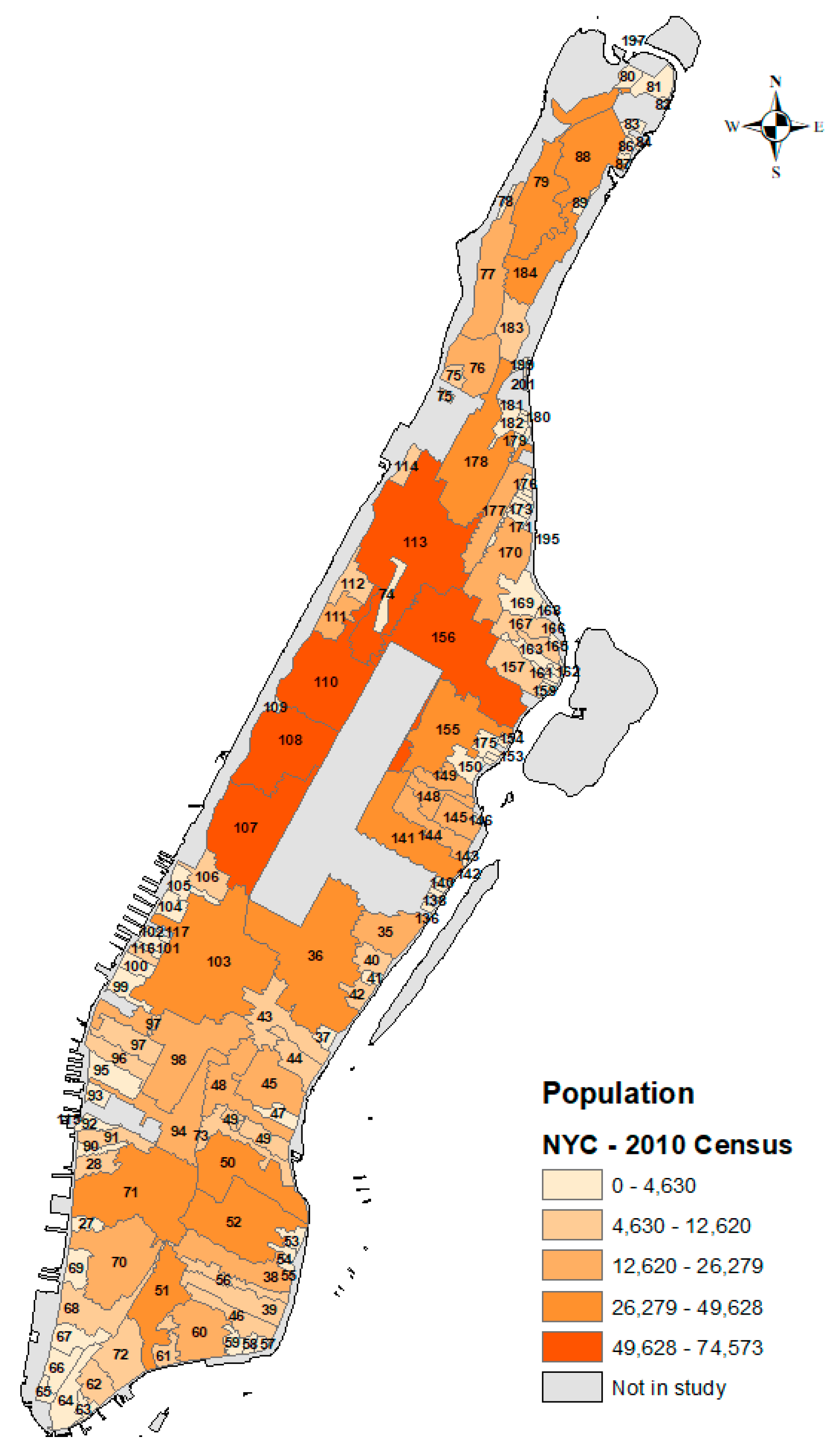
We base this work on the 140-stormwater sub-basins designed by the New York Environmental Protection Agency (NYEPA) [
13]. We use a DEM derived from the 2010 Light Detection and Ranging (LiDAR) data at a 0.30-m horizontal resolution with a vertical RMSE between 9.5 cm and 33.08 cm [
14].
Figure 1 shows the 140 sub-basins and population densities of each of the areas.
2.1. Flood Map Database
The database is a collection of flood maps for each one of the 140 sub-basins of our study area. This map collection provides a geographical approximation of flooded areas at different rainfall volumes. It also reduces computational time because most possible flooding scenarios have already been pre-prepared.
In order to build this database, we acquired elevation, man-made structures (buildings, streets, sidewalks), and land cover information from the NYC Open Data repository [
14]. All data were processed in ArcGIS 10.4 and Python to facilitate automation. We created separate elevation, structures and land cover raster files for each of our sub-basins. In this manner, each sub-basin can be treated as a sub-area of study.
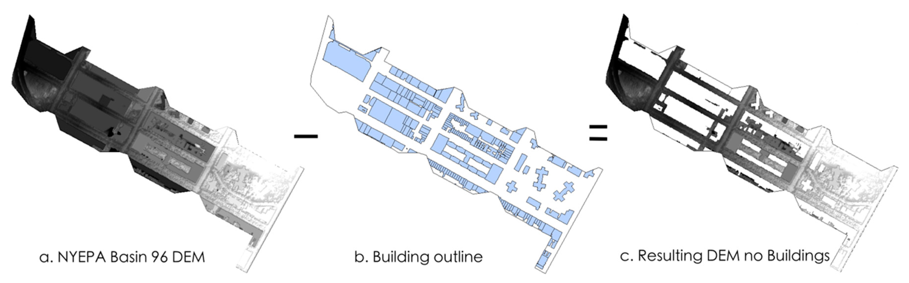
The original DEM contains elevation values of all buildings and structures, but our hydrological analysis is limited to that of the land surfaces other than buildings. Therefore, we subtracted the building footprint for all 140 sub-basin DEM files. We also assumed that the rainwater on the rooftops is collected through the building storm drainage and directly transferred to the stormwater system.
Figure 2 depicts a sub-basin DEM before and after building/structure subtraction.
We calculated the total sub-basin area
; the length of the streets
LSi; the land cover types (impervious
, bare soil
, and green areas
; and the lowest and highest topographical points in each sub-basin. The approximate number of storm sewer inlets
NCi was derived using Equation (1) below, where
S is the spacing between storm inlets in the catch basin and NB is the number of sub-basins in the study area (NB = 140). It is important to note that for our particular area of study, S is based on the NYEPA sewage layout, which includes one inlet at each corner of major intersections and equally spaced inlets along streets. However, we used Equation (1) below to estimate the number of inlets in the area. Then, all information for each sub-basin was transferred to an Excel file.
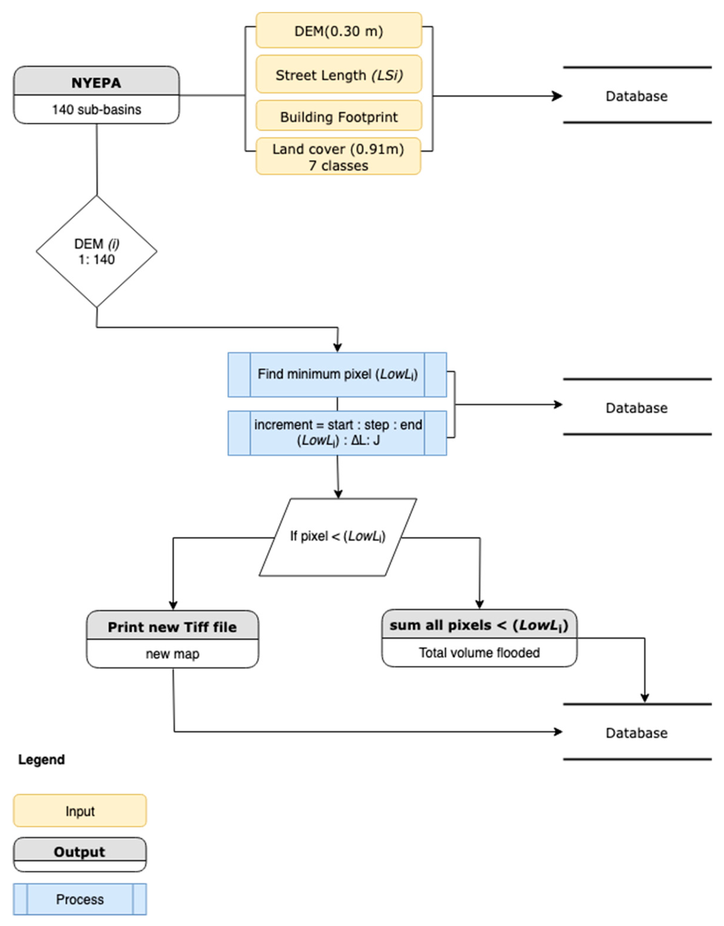
Starting at the lowest topographic points for each sub-basin DEM file (i), each elevation increment (ΔL) is considered a new flood level Li,j. For example, the lowest DEM topographic pixel point at NYEPA Basin-96 is 2.12 m, this is,
. At an interval
= 15.25 cm, the next level,
is 2.27 m,
is 2.42 m, and so on. We calculated flooding volumes (V) and the total flooded area for each flood level in a new map. In our example above, the total flooded area at
= 68.5 m
2,
= 577 m
2,
= 1,260 m
2, etc. Equation (2) explains the computations in this process.
where
represents the number of pixels in the sub-basin,
is the pixel level,
the pixel area, and
where
is the lowest topographic point at sub-basin
i,
Li, j.
The final database is then composed of a table of records containing descriptive information about each sub-basin (permeable, not permeable, land cover, etc.), corresponding flood levels, flooded area, runoff volume, and a resultant flood map. The flow chart in
Figure 3 shows the complete process implemented for building the database.
2.2. Rainfall-runoff Model
The rainfall-runoff model presented here follows the concept of mass balance in a catchment area and includes physical processes of rainfall, infiltration, and storm inlet flow. Here, this concept is applied to each pixel of the DEM raster. The volume of rainfall received at each pixel within a time period represents the inputs. The outflows are represented by infiltration and street inlet flows but exclude evaporation. Input and outflows are subtracted to determine the remaining flooding volume at the end of the storm period. The total flooding volume for the area is the sum of the runoff volume for all pixels.
The use of pixel-based mass balance allows for temporal and spatial rainfall intensity variations. It also allows for infiltration differentiation according to land cover type. For pixels containing inlets, we determined storm street inlet flow by incorporating Armal and Al-Suhili 2019 [
15] proposed methodology. This methodology accounts for inlet blockages and it is explained below. In addition, we used Horton’s infiltration model to determine the time effect from initial infiltration until threshold rate.
The innovative approach presented here relies on the coupling of the model and the flood map database. The flood maps are easily accessible throughout the storm event as well as during the recession period. We implemented the following steps for the creation of model:
- (1)
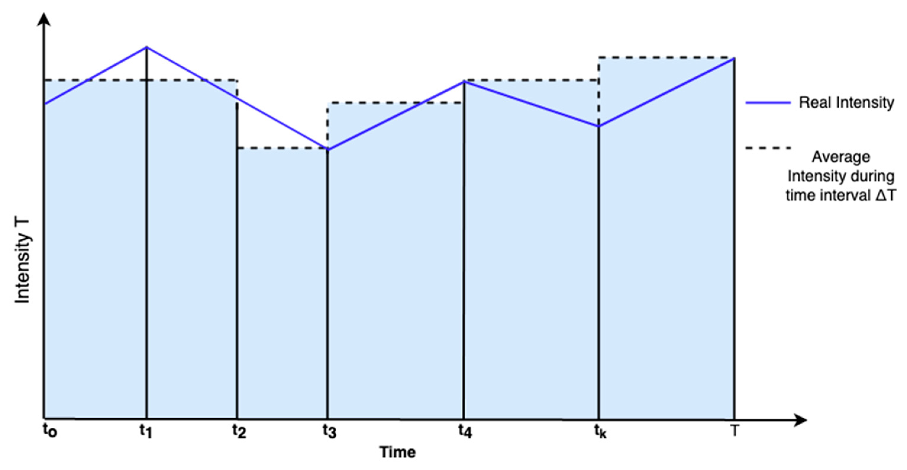
For any expected rainfall event, the total period of storm T and its rainfall intensity
time variation is shown on the storm hyetograph in
Figure 4.
- (2)
The user selects time interval
ΔT, which in turn selects the number of time steps
and flood maps as per Equation (3).
Maps are displayed for each time interval as shown in Equation (4).
where
tk represents time from the beginning of the storm event up to
k intervals of
ΔT.
The flooding event simulation can be extended to cover the storm recession period (i.e., the period after the rainstorm ends, up to the time where the runoff water is fully drained by the storm sewer network). In this case, Equation (4) is extended as follows:
where,
is the number of time steps
, for the recession period, i.e., after the rain stops, as selected by the user.
- (3)
The rainfall intensity during any period,
is obtained by averaging the intensities at those times. The following equation can be used for the rainfall intensity during the total time of the storm event and recession period.
where
Rk is the average intensity over time (
tk,
tk-1).
- (4)
Using rainfall, infiltration and the storm inlet flow processes, runoff volume at any time
is estimated using the following equation:
where V
k, and V
k-1 are runoff volumes at time intervals t
k and t
k-1 respectively, D
k represents the volume of water drained through the street inlets of the storm sewer system during time interval
, as per Liu et al. 2015 [
16], and Inf
k represents the infiltrated volume during the time interval as:
where f
b and f
g are the average infiltration rates for bare soils and green areas.
The equation below is used for calculating the inlet flow as water intake rate:
In order to simulate inlet flow partial blockage, and its resulting backflow, we modified Equation (9) into Equation (10) by introducing the
factor as proposed in Armal and Al-Suhili 2019 [
15]. Here,
fluctuates between −1 and 1 during the simulation time interval. 1 represents a full inlet, at full inlet inflow capacity. A partial blockage results in a number between (1 and 0). 0 represents a full blockage, and values between (−1 and 0) represent a partial backflow while a value of −1 represents full backflow. A linear beta-time variation is assumed with negative trend (slope) and an initial value of 1, (i.e., beta decreases from 1 to −1 with time). The slope value is first assigned according to the topography of the area and the location of the inlet. We verified the assigned slope value using the head variation with time in the pixels that include an inlet. We assumed that the inlet starts back flowing when there is an increase on the head (flood depth) that is not related to the amount of rainfall.
where
Q is the inlet discharge flow m
3s
−1,
w is the area of the inlet m
2 C represents the orifice coefficient,
g is the gravitational acceleration,
h is the allowed water storage head of an inlet, and
k is orifice obstruction coefficient to account for interception of outlet screen racks. With this equation, then we can estimate the inlet volume D:
- (5)
The simulation starts by setting the initial runoff volume, i.e., at t = 0, as V0 = 0. The system proceeds to estimate Vk for different k-values. Then, at each appraised volume, the model calls the map database and displays the map that closely matches the projected runoff volume.
The rainfall-runoff model simulation process uses the above calculations at selected time intervals during the storm. Infiltration rates are determined using Equation (12), Horton’s equation. The storm sewer inlets are determined using Equation (10). The initial value of is 1, and it is assumed to reduce with time during the simulation period. A negative value is adopted if the total storm interval lasts long enough to produce backflow. The inlet flow head, h, is assumed to increase linearly with time. Accuracy of the simulation is, of course, affected by time variations of these factors. The actual and the simulated runoff depths are expected to have small differences, but they do not affect our objective of pre-identifying flood areas. The expected damages and consequences of severe floods, i.e., 40 cm or higher, will not be much affected by a few centimeters of flood depth.
3. Results
In this work, the sub-basin database and the rainfall-runoff model work together to reduce computational time and provide a map of the flood area. The database informs the model about the specific conditions (paved areas, permeable areas, land cover type, total area, etc.) of each sub-basin and subsequently delivers the appropriate flood map of the area.
In the following pages, we assess the capability of the rainfall-runoff model to forecast flooding areas in an extreme rainfall event. We evaluate the efficacy of the pre-prepared database in relation to the rainfall-runoff model and its capability to select the best suitable flood map and last, we apply the system functionality to a case study in the area.
3.1. Database
The full assembly of the database results in a set of tabulated information as shown in
Table 1 and a set of corresponding maps as shown in
Figure 5.
Figure 5 below shows four levels corresponding to basin number 53 located on the lower East side of Manhattan, each one of these maps corresponds to the first four rows of information in
Table 1.
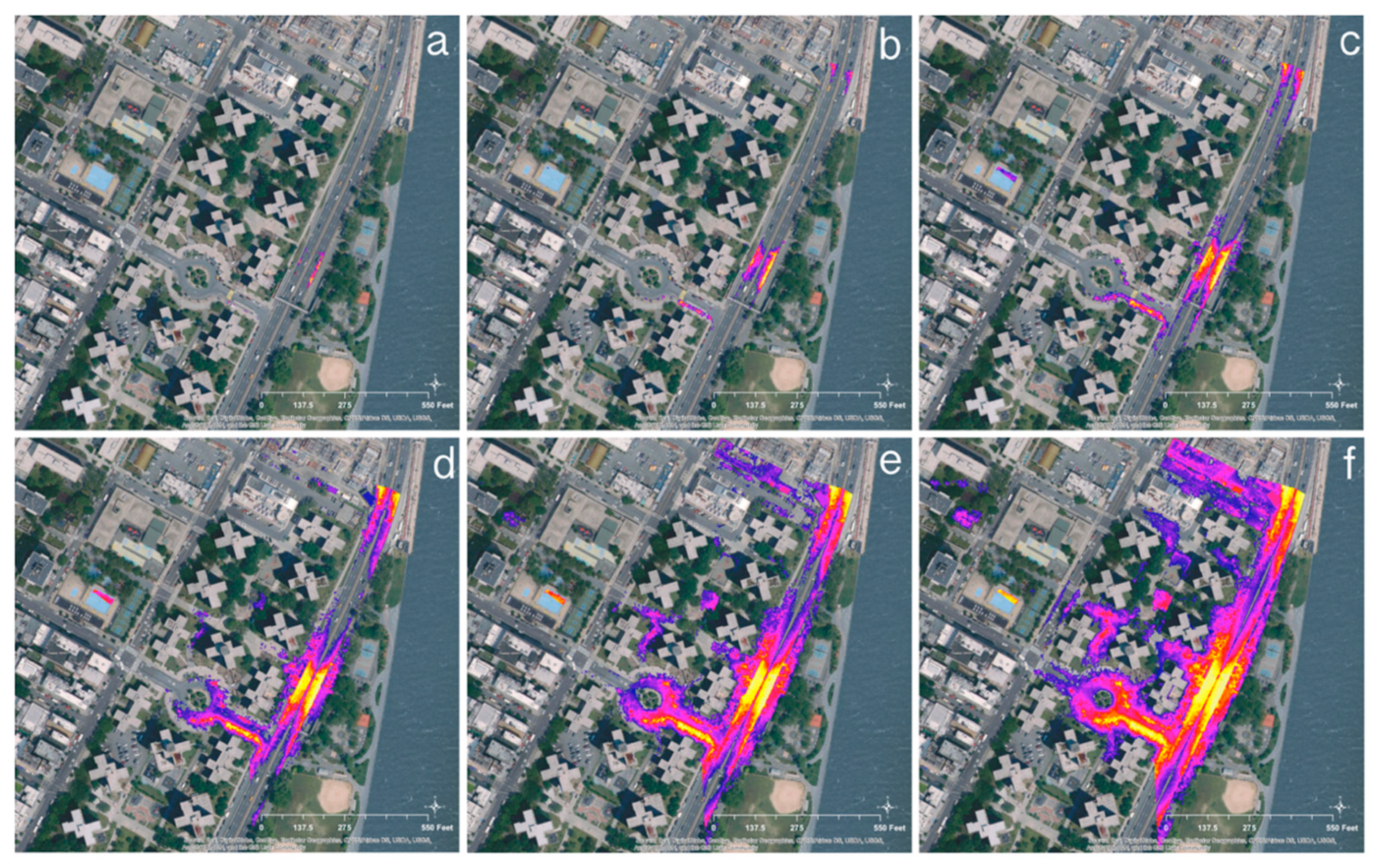
As the user selects the sub-basin of interest and inputs the expected amount of rainfall and it’s duration, several maps in pdf format are displayed or printed for the area as shown in
Figure 6 below.
3.2. Case Study—Extreme Rainfall Event May 5, 2017
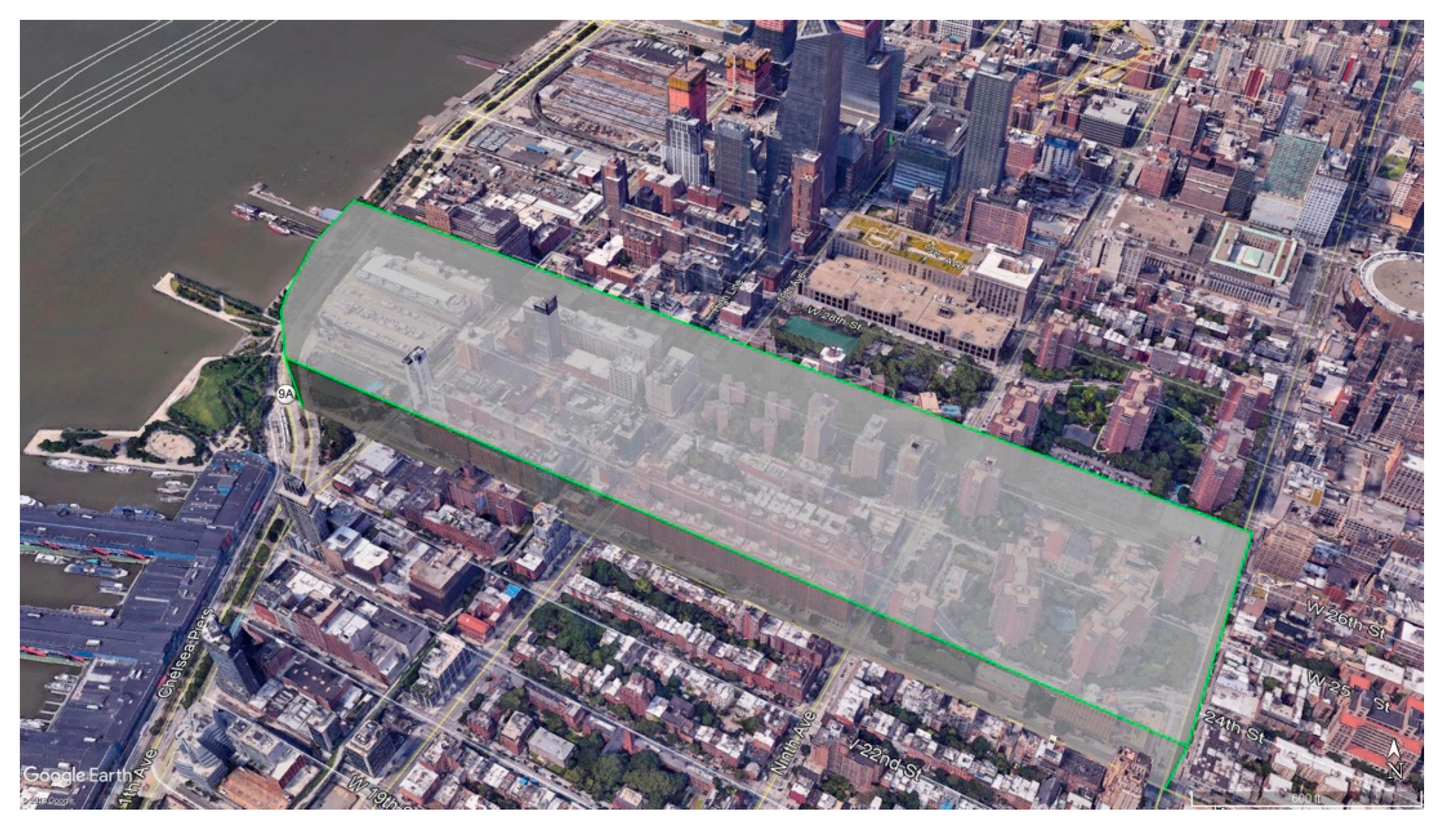
The May 05, 2017 storm and the corresponding flood that affected Manhattan Island, NY, is used as a case study for the model. The estimated average intensity of the storm was 15.3 cm/hour. This averaged intensity is distributed over a 15-min duration. The specific sub-basin location in Manhattan is identified as Basin-96 in the NYEPA designation. The basin encompasses the area between 12th Avenue in the West, 8th Avenue in the East, 23st in the South and 26st in the North.
Figure 7 below shows the total basin area.
The basin total area is 244,713 m
2, the pervious area is 15,623 m
2, and the total street length is 5124 m. The soil type of this area indicates the following Horton’s infiltration parameters for the application of time variant infiltration rate: fo = 0.1423 cm/min, ff = 0.0021 cm/min, and k = 0.07 1/min.
where
is the infiltration rate at time t;
is the initial infiltration capacity,
is the final infiltration (threshold value) capacity,
is the decay constant, and
is time. There are 34 estimated storm sewer inlets in the basin. The head of each inlet is assumed to be 0.05 m at the start of the storm and increase at a linear rate to a threshold value of 0.1 m. The inlet flow was deduced using the reduction factor
as mentioned above. With this information, the model application resulted in the outputs shown in
Table 2 below.
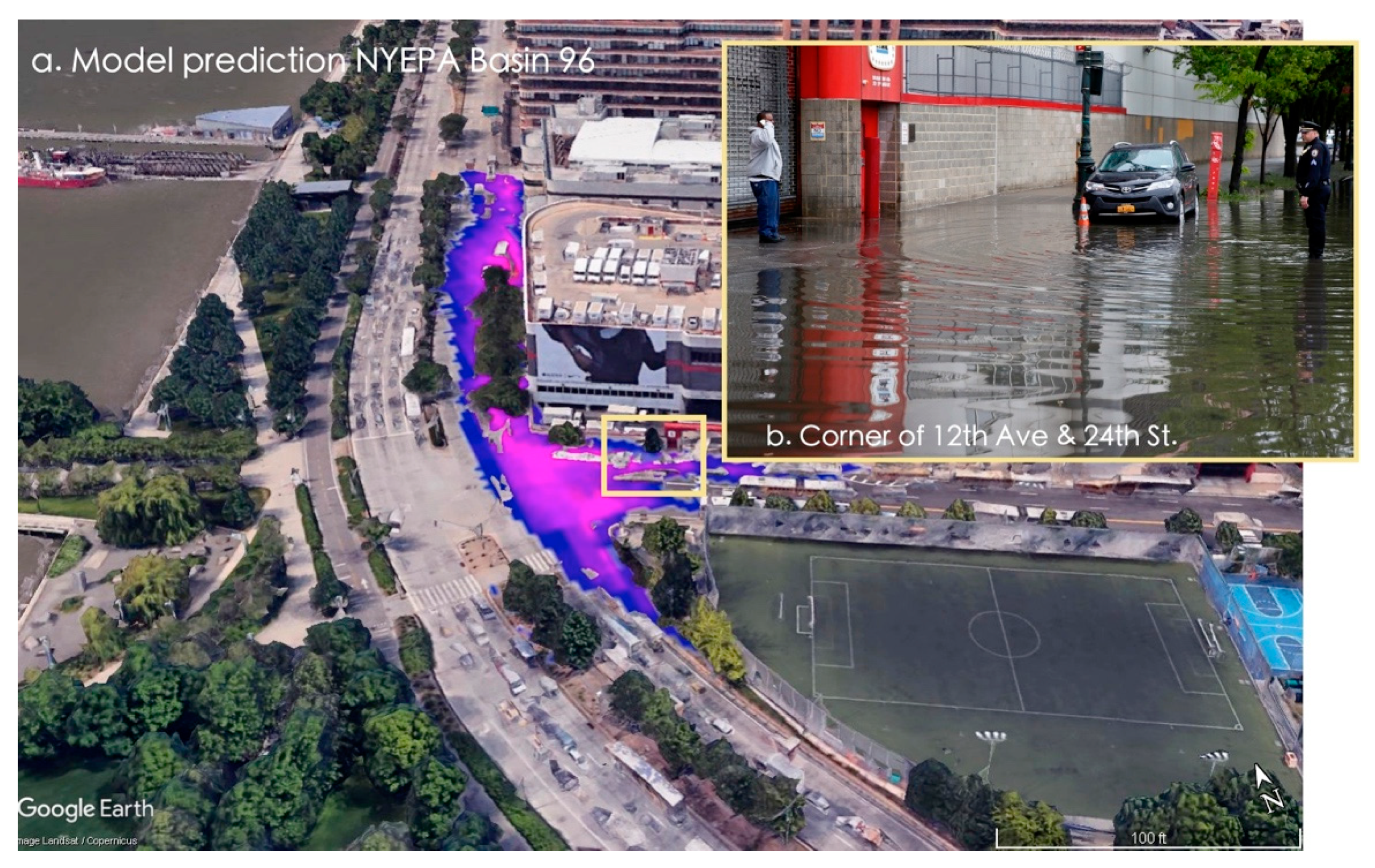
The model searches the database to find the closest flooding map that represents the actual runoff volume. For our case study,
Figure 8a. shows the map corresponding to the rainfall event. A picture of the corner of 24th St and 12th Avenue (area within NYEPA Basin 96) shows actual flooding during the May 5th storm in
Figure 8b. This area corresponds to the West Side Highway (12th Avenue), a major transportation way in Manhattan. As reported by numerous media outlets [
17,
18] the heavy downpour caused several road closures around the metropolitan area. The National Weather Service reported closures between 20th and 30th streets on the West Side Highway at around 1:40 PM due to flooding [
19].
The study case shows that the system can generate several flood level maps that are congruent with actual flooding. The picture taken of the flooded area at the moment after the storm coincides with the area assigned as flooded by the model. The case study also shows that the system is consistent with mass conservation at reasonable computational time.
As the average intensity of the storm is an estimate, its value may impact the model’s precision. Nevertheless, since our goal is to quickly determine the area that is most likely to be flooded, the system rapidly computes volumes and chooses the corresponding flood map. Results for this case study show that for a 15-min storm period, subdivided at 5-min intervals, the total computational time is 3 min.
3.3. Parameter Sensitivity Analysis
Sensitivity analysis is useful for finding the percentage change variation in the estimated volume. It helps us define the level of accuracy required for setting temporal and spatial variations of parameters in the model. Specifically, to detect whether their variation is linear or non-linear and if these changes are relatively high or low.
Table 3 below shows percentage reductions in runoff volume at the end of the storm due to variations of different parameters.
Parameter sensitivity analysis showed the following. With respect to the low head time variation for the storm inlets, the change in head variation was set at 0.01 cm/min as reference value and time interval was set at 5-min. We tried different variations at 0.015, 0.02 and 0.025 cm/min. Results showed an approximate linear variation at a rate of approximately 3.4 percent increase. Regarding variation of the threshold infiltration rate, the reference value was set to 0.048 cm/min and it was reduced to 0.04, 0.032 and 0.26 cm/min. The time interval was also set at 5-min. Results indicated a non-linear variation of runoff flow with a small (0.76 to 0.52) percent increase. With respect to the effect of the number of storm inlets, we used 34 as reference value and reduced it by 2 at each 5-min interval. We also observed a non-linear variation in this parameter. The percentage increase in runoff flow ranged between 6.25% and 5.55%. Finally, concerning the storm inlet flow reduction factor effect, time variation was found to be non-linear with a range between 11.7 and 8.33. This indicates that variations of this parameter are very sensitive and need further investigation for future applications.
4. Discussion
This paper introduces a coupled GIS-based model and map database that simultaneously works to facilitate the urban flooding management process. The purpose of this coupling is so that potential flooded geographically areas can be determined before the storm. Given the complexity of all model types (physical, semi-physical, image processing, etc.), this approach was developed with some simplified assumptions. Evaporation, for example, is not considered as a variable in the model since its value during a storm event is not significant.
We underline that various assumptions and variations of the many parameters in the model will affect accuracy. The accuracy of inundation depths in this model for example, relies solely on the calculation of the rainfall amount, infiltration rate, and the storm inlet flow processes. In addition, the extent of the flooded area is considered to decrease with distance from the maximum head or inundation depth. Nevertheless, we achieve our objective to present a system that can quickly simulate flooded areas before the storm.
Our study case demonstrates that computational time is relatively short. The system took 3 min to complete calculations for three time intervals of a 15-min storm. We also tried five different intervals, at 3 min each, for a 15-min storm. The system completed all the calculations in 4 min. The interval time and the processing time are not linearly correlated, but overall, compared to other available systems, this model can be used as a quick reference.
4.1. Limitations
(1) Verification limitations: depth verification is not presented in this document and is needed for future fine-tuning of the model. At this time, the model is devoted to finding areas prone to urban flooding and their extent.
(2) Homogeneous rainfall: as spatial variations of rainfall must be considered, the system here presented is completely reliant on the availability of detailed rainfall forecasts and rain gauges.
(3) Temporal rainfall distribution: the rainfall time-intensity variation is not considered, and consistent average rainfall intensity is assumed during the storm time interval.
(4) Data limitations: the presented model is a data driven system that relies on the accuracy of data inputs. In this case, we have used a 0.30 m resolution LiDAR DEM of NYC but other relevant information such as land use and land cover types are not yet available at such resolution.
(5) Sub-basin-based inundation: in this study, flooding is calculated separately for each sub-basin. Uneven or unrealistic flooding conditions may be encountered at each sub-basin boundary area.
(6) River flooding: based on the limitations and criteria that the system is built on, the system is not appropriate to use for river flooding.
4.2. Future Directions
Validation with a future rainfall event needs to be studied to compare model results to real flood depth spatial distribution. Furthermore, as sensitivity analysis demonstrates, the reduction factor variation needs further analysis as it exhibited a high non-linear variability. As we fine-tune the system, it will be extended to the other boroughs of New York City.
5. Conclusions
We propose an urban flash flood alert tool that couples a rainfall-runoff model with a flood-level map database that expedites the alert system process. The pre-prepared flood maps database can be used for a quick identification of the areas prone to flooding when coupled with the rainfall-runoff model, with very short processing computer time compared to other models. Our approach presents reasonable flooding results for the sake of quick preparedness. We expect that the resultant maps can inform authorities and citizens about expected conditions in the streets and on the roads in the city as a storm approaches. It is our hope that decisions, such as closing traffic in a particular area, can be aided by this system.
The spatial flood depth distribution of the flooded area can be estimated at any time within the storm interval using ArcGIS. Unfortunately, this flood runoff depth spatial distribution cannot be verified due to the lack of spatial depth measurements during the storm event of the case study, and hence left for future research. As for the current document, the objective is only to develop a model for identifying areas prone to flooding and the extent of the flood regardless of the depth, i.e., any area covered by residual water.
Sensitivity analysis of the model showed that the storm inlet flow parameter exhibits a linear variation of (3.4%). The threshold infiltration rate, the number of storm inlets and the storm inlet reduction factor showed a non-linear variation. However, the reduction factor variation showed a high non-linear variation, as it is a very sensitive parameter. For this reason it is necessary to further research the effects of this factor in relation to the overall model. Perhaps in the future, with the acquisition of real-time depth data from satellites, this factor can be calculated with more precision.
Lastly, in spite of the limitations posed by the rainfall spatial and temporal variations, the model was developed in such a way that these variables could easily be included using GIS-Excel data files in future work.


