Article

Effects of Bias-Correcting Climate Model Data on the Projection of Future Changes in High Flows

Department of Hydrology, Water Resources Management and Water Protection, Leichtweiß-Institute for Hydraulic Engineering and Water Resources, Technische Universität Braunschweig, Beethovenstr. 51a, D-38106 Braunschweig, Germany
*
Author to whom correspondence should be addressed.
Hydrology 2019, 6(2), 46; https://doi.org/10.3390/hydrology6020046
Submission received: 23 April 2019 / Revised: 24 May 2019 / Accepted: 28 May 2019 / Published: 4 June 2019

Abstract

:
Bias-correction methods are commonly applied to climate model data in hydrological climate impact studies. This is due to the often large deviations between simulated and observed climate variables. These biases may cause unrealistic simulation results when directly using the climate model data as input for hydrological models. Our analysis of the EURO-CORDEX (Coordinated Downscaling Experiment for Europe) data for the Northwestern part of Germany showed substantial biases for all climatological input variables needed by the hydrological model PANTA RHEI. The sensitivity for climatological input data demonstrated that changes in only one climate variable significantly affect the simulated average discharge and mean annual peak flow. The application of bias correction methods of different complexity on the climate model data improved the plausibility of hydrological modeling results for the historical period 1971–2000. The projections for the future period 2069–2099 for high flows indicate on average small changes for representative concentration pathway (RCP) 4.5 and an increase of approximately 10% for RCP8.5 when applying non-bias corrected climate model data. These values significantly differed when applying bias correction. The bias correction methods were evaluated in terms of their ability to (a) maintain the change signal for precipitation and (b) the goodness of fit for hydrological parameters for the historical period. Our results for this evaluation indicated that no bias correction method can explicitly be preferred over the others.

1. Introduction

An intensification of the hydrological cycle due to climate change is likely, but varies in dependence of the geographic region and spatial scale [1]. This implies precipitation, flood intensities and frequencies as well as the occurrence and magnitude of droughts and low water situations. Changes in intensities and frequencies of precipitation related to global warming investigated both on the global [2] and regional scale [3,4,5] compared climate impact projections of river floods in Europe under climate change. They concluded that flood risk will consistently increase in most of Central and Western Europe. But in addition to this, investigations on smaller spatial scales are needed to identify flood endangered areas due to regional varying effects of climate change [6]. These studies are necessary in order to develop specific adaptation measures of public authorities and local governments [7].
When assessing the impacts of global change on mesoscale catchments, the general procedure is the application of a chain of several models/steps: (1) general circulation models (GCM), (2) regional climate models (RCMs) or statistical downscaling, (2b) bias-correction (BC) and (3) hydrological models. Due to the coarse spatial resolution of GCMs of 1–2° [1], the direct application of these data for hydrological models is only useful in large-scale catchments. At mesoscale level, step (2) is necessary in order to consider local climate variability. The background of BC is the often large deviation between RCM output and locally observed values for historical periods. Concerning precipitation, which is the main driver of hydrological processes [8], there are large deviations in the simulated intensity and frequency of precipitation events [9]. In general, BC methods are transfer functions with different complexity based on statistical analyses [10,11]. A comprehensive overview of various BC methods is given by [12].
Within the framework of the German research project “KliBiW” (Global Climate Change—Consequences for the inland water resources management) possible future changes in discharge in the federal state of Lower Saxony are quantified. The ensemble of climate model data comprises projections based on the SRES A1B scenario and on the RCP (representative concentration pathway) scenario RCP8.5. The previous results of this on-going project showed an increase in both flood risks and low flow events in the course of the 21st century [7,13]. The results of the project raised the question of the contribution of BC on the future projections for hydrological parameters. For this reason, additional analyses were carried out applying different BC methods.
The advantage of bias-correcting climate model data prior to using them as input for hydrological models is the improved representation of observed hydrological variables such as discharge or groundwater recharge by model simulations. Applying non-corrected climate model data often leads to the simulation of hydrological processes in unrealistic magnitudes. On the other hand, it is argued that BC adds another source of uncertainty to the model chain. Furthermore, BC mostly impairs the alteration of the relations among climate variables and feedback mechanisms. The application of BC for the historical period as well as for a future period assumes that the bias is constant over time in a changing climate, which is not assured [8]. Lafon, T. et al. [14] investigated the robustness and the effectiveness of different BC methods. They found that the parameters of the BC may be sensitive to the time period for which the BC parameters were calibrated.
Huang et al. [15] investigated the performance and impacts of BC on flood projections in Germany. They applied the distribution mapping method on two different RCMs. In their study, 75% of the change directions (positive/negative) of flood discharge were not influenced by BC. Teng et al. [16] applied four different BC methods on precipitation. Their results showed that BC did not affect the signals in precipitation means, but could generate additional uncertainty on change signals of high precipitation, which influences simulated discharge. Most studies focus on the two variables temperature and precipitation when bias-correcting climate model data for hydrological impact studies [12,15].
The aim of the study at hand is the contribution to the following key points:
  • Sensitivity analysis for assessing the necessity of bias correcting various climate variables when using climate scenario data as input for hydrological models.
  • Projecting future changes in high flow parameters in six medium-scale catchments in the Northwestern part of Germany.
  • Evaluating the performance of BC methods of different complexity.

2. Data and Study Area

2.1. Climatological Data

2.1.1. Observational Data

The observed meteorological input data (precipitation, mean, minimum and maximum temperature, relative humidity, global radiation and wind speed) was available on a daily time step for the period 1951–2015 from the Lower Saxony Water Management, Coastal Defence and Nature Conservation Agency (NLWKN). Data from 771 stations for precipitation and 123 stations for the other meteorological variables was used to generate 1 × 1 km gridded data fields for Lower Saxony by means of geo-statistical analyses. This was executed by Institute of Water Resources Management, Hydrology and Agriculture (WAWI) of the Leibniz University of Hannover in the framework of the research project KliBiW. These fine-resolution grids were used as input data for the calibration and validation of the hydrological model.
For the comparison with the RCM data for the historical period 1971–2000, the observational 1 × 1 km grid was aggregated to a 10 × 10 km grid. In the following, this grid data is referred to as observational data Xobs.
Observed discharge data, Qobs, was available on a daily basis for at least the year 1977 up to 2011 from the NLWKN.

2.1.2. Coordinated Downscaling Experiment for Europe (CORDEX) Data

The RCM data were obtained from the CORDEX (Coordinated Downscaling Experiment for Europe) project [17]. The 17 GCM/RCM combinations, hereafter referred to as climate scenarios, were composed of six different GCMs and six different RCMs (Table 1).
In this study, two RCP scenarios were considered: RCP4.5 and RCP8.5. The name of the RCP refers to the projected additional radiative forcing in W/m2 [18]. Additionally, historical runs for the climate scenarios were also available. All climate scenarios have a spatial resolution of 0.11° (about 12.5 km) and a temporal resolution of one day.
Most of the climate variables needed by the hydrological model were available from the CORDEX project. Relative humidity was not provided by all climate scenarios. It was generally calculated in dependence of specific humidity and daily mean temperature [19] as the ratio of actual water vapor pressure to saturated water vapor pressure. Before further processing, a reprojection of the CORDEX data was necessary in order to comply with the coordinate system and resolution of Xobs (see Figure 1). This was done using the inverse distance method with the consideration of three neighbours.

2.2. Study Area

The study area comprises six mesoscale catchments with spatial extends of 309 to 1731 km2 in the Northwestern part of Germany (see Figure 1). The region is mostly flat with a mean elevation of the catchments between 45 and 210 m above sea level.
The annual precipitation for the period 1971–2000 varies between 620 and 820 mm for the six catchments. The annual mean of temperature is similar in all catchments (8.6–9.6 °C).
The texture of the soil in the catchments Emlichheim and Hellwege is sandy whereas in the catchments of Derneburg and Wunstorf, the soil texture is dominated by silt. In Harxbüttel and Bramsche, loams with both fine and coarse texture size can be found.
The catchment land use is mainly agricultural with winter crops and corn being the predominant crop types.

3. Methods

3.1. General Procedure

Projections of 17 climate scenarios and two RCP scenarios for the future period 2070–2099, Xfut, as well as corresponding data for the historical period 1971–2000, Xhist, were used as input for the hydrological model PANTA RHEI in order to identify hydrological climate change signals with a focus on high flow parameters. High precipitation values being a crucial factor for high flows are also investigated in terms of climate change signals. All time periods are based on the hydrological year and comprise 30 years (e.g., 11/1970–10/2000). The influence of BC was assessed by correcting climate variables with different methods and comparing the resulting parameters for the historical period and the climate change signals with those obtained by non-corrected climate scenario data. Non-corrected climate scenario data are referred to as Xhist,orig/Xfut,orig, bias-corrected data are Xhist,bc/Xfut,bc.
For the computation of climatological parameters and the corresponding climate change signals, all grid cells with the center within the catchment boundaries or within a distance of maximum 5 km from the catchment boundaries were considered. The number of grid cells per catchment varied between 6 and 31. The total number of grid cells for all catchments was 93.
First, the necessity of the application of BC for the different climate variables was identified by comparing Xhist,orig to Xobs in terms of annual mean values and monthly deviations. The number of wet days and parameters for high precipitation events were also considered. In accordance with the majority of studies reviewed [20,21] a threshold of 1 mm/d was applied to define a wet day (WD1). In terms of high precipitation events, the 95% percentile of (a) daily precipitation on wet days (P95) and (b) the 3-day precipitation sum above 3 mm (P95d3) were compared. The overall result of the comparison between Xhist,orig and Xobs is calculated as the average of all 93 grid cells. Simulation results of the calibrated hydrological model forced with both Xobs and Xhist,orig were analysed regarding the deviations in average discharge (MQ) and the mean of annual maximum discharge (MHQ). Hereafter, the simulated discharge applying Xobs/Xhist,orig/Xhist,bc is referred to as Qref/Qhist,orig/Qhist,bc. Discharge simulations for the future period are correspondingly abbreviated with Qfut,orig and Qfut,bc.
The BC effects on the simulation of high flow parameters during the historical period were assessed by comparing the parameters MHQ and flood events with a 100-year return period (HQ100) of Qref and Qhist,bc. The parameter HQ100 is estimated using the Gumbel distribution and L-Moments for the parameter estimation of the function. In terms of the climate change signals, the parameters P95d3 and MHQ were compared. For P95d3, the mean value of all grid cells was used, for MHQ, it is the area-weighted mean of all six catchments.

3.2. Hydrological Model PANTA RHEI

The hydrological model PANTA RHEI has been developed by the Department of Hydrology, Water Management and Water Protection, Leichtweiß Institute for Hydraulic Engineering and Water Resources, University of Braunschweig in cooperation with the “Institut für Wassermanagement IfW GmbH”, Braunschweig [22]. It has been successfully applied for scientific questions in numerous national and international projects [7,23,24]. Furthermore, PANTA RHEI is applied in the operational flood forecast of the Federal State of Lower Saxony, Germany [25].
PANTA RHEI is a deterministic, semi-distributed, physically based hydrological model with a three level spatial disaggregation scheme: catchment, subcatchments and hydrotopes. Within a subcatchment, hydrotopes are homogeneous regarding the soil type and land use type.
The internal temporal discretization of PANTA RHEI is one hour. However, the time step of climatological input data can be different. For this study, discharge data were evaluated on a daily basis. A detailed description of PANTA RHEI is given by [26].

Calibration and Validation

The six catchments of the study area were calibrated and validated with observational climate and discharge data for the period 1971–2011. The first 20 years were used for calibration and the last 20 years for validation. Due to data availability, for the gauges Derneburg and Harxbüttel, a slightly shorter period was used.
The calibration was done semi-automatically applying the lexicographic strategy developed by [26] using four criteria: the percentage deviation of the total discharge volume, the mean monthly deviation of discharge, the Nash–Sutcliffe efficiency [27] and the root mean squared error (RMSE) of the maximum annual discharge (HQa). The mean monthly deviation is calculated by the absolute values of percentage deviations.
The Nash–Sutcliffe efficiencies for both periods range between 0.79 and 0.91 with a mean of 0.83 for calibration as well as for validation, which can be denoted as values of high quality. The deviation in total discharge volume amounts to a maximum of 8.6% during both periods. The mean monthly deviation of discharge varies between 3% and 16% and is slightly higher for the validation period for all catchments.

3.3. Sensitivity Analysis for Climate Variables

The sensitivity of discharge in dependence of climate variables was carried out for all climate variables that serve as input for the hydrological model. The variables of Xobs were altered in order to assess the impact of changes in one variable on the simulation of discharge. The alteration of Xobs was carried out either by multiplication with a factor (wind speed, humidity, radiation, precipitation) or by addition of a value (temperature). The level of change is derived from the deviations between Xhist,orig and Xobs for each variable during the historical period. Therefore, three sensitivity levels (SL) were defined. The SL take into account the mean deviations and the standard deviation of the deviations between Xhist,orig and Xobs (see Equations (1)–(6)) for the two examples of precipitation and temperature).
P S L 1   ( d ) = P o b s   ( d )     μ s   ( P h i s t , o r i g ) μ     ( P o b s )
P S L 2   ( d ) = P o b s   ( d )   (   μ s   ( P h i s t , o r i g )   +   σ s   ( P h i s t , o r i g ) ) μ     ( P o b s )
P S L 3   ( d ) = P o b s   ( d )   (   μ s   ( P h i s t , o r i g )     σ s   ( P h i s t , o r i g ) ) μ     ( P o b s )
T S L 1   ( d ) = T o b s   ( d ) + μ s   ( T h i s t , o r i g )   μ     ( T o b s )
T S L 2   ( d ) = T o b s   ( d ) +   μ s   ( T h i s t , o r i g ) μ   ( T o b s )   + σ s   ( T h i s t , o r i g )
T S L 3   ( d ) = T o b s   ( d ) +   μ s   ( T h i s t , o r i g )   μ   ( T o b s )   σ s   ( T h i s t , o r i g )
where P is precipitation, T is temperature, d is the day, µ is the mean of observational data, µs and σs are the mean and the standard deviation of climate variables of all climate scenarios considered.
The adjustment of the variables wind speed, humidity and radiation was undertaken analogous to that for precipitation. In terms of relative humidity, values that amounted to >100% were set to 100%. The daily minimum and maximum temperature were adjusted with the same deltas as mean temperature, so that the temperature amplitudes of the Xhist,orig were not changed.
One climate variable was altered according to one sensitivity level for each simulation run of the hydrological model, while Xobs was used for the other input variables. In addition to these local sensitivity studies, one global sensitivity simulation run was carried out with alterations of all variables according to SL1.
The sensitivity of discharge in dependence of climate variables was evaluated for the two parameters MQ and MHQ.

3.4. Bias Correction for Hydrological Modeling

The main focus when comparing different BC methods was on precipitation as it is the most critical factor for the deviations between Qref and Qhist,orig (see Section 4.2). Various methods with different complexity were applied to Phist,orig. All other climate variables were corrected with the linear scaling method.
The following short description of BC methods therefore focuses on the adjustment of precipitation although some methods are also applicable to other climate variables. As a part of some methods, the wet-day frequency is adjusted, as it is overestimated by most of the climate scenarios. In this study, this is generally done by applying the approach described by [21] as part of the local intensity scaling (LOCI) method with a 1mm threshold for a wet day. In contrast to a 0 mm threshold, which is used by [12], this also allows the adjustment in case that the wet-day frequency is underestimated by climate scenarios. In our study, this method is part of the BC methods LOCI, power transformation and distribution mapping. For all BC methods applies that Xfut,orig, is corrected the same way as the corresponding data Xhist,orig and all corrections are carried out on a monthly basis.

3.4.1. Linear Scaling

Linear scaling is a well-established BC method. The adjustment is made based on the difference in monthly mean values between Xobs and Xhist,orig. A correction factor calculated out of these differences is applied to Xhist,orig and Xfut,orig either by summation (temperature, Equation (7)) or multiplication (all other variables, see Equation (8) for the example of precipitation):
T b c ( d ) = T o r i g ( d ) + ( μ   ( T o b s ( i ) )   μ ( T h i s t , o r i g ( i ) )   )  
P b c ( d ) = P o r i g ( d ) μ   ( P o b s ( i ) ) μ ( P h i s t , o r i g ( i ) )  
where “bc” indicates the bias corrected data, µ is the mean and i is the month (1…12).

3.4.2. Local Intensity Scaling (LOCI)

The LOCI correction, is described in detail e.g., by [21] and implies the adjustment of the wet-day frequency. This is done by defining a wet-day threshold (WDT) from Phist,orig in such a way that the number of days in that time series matches the number of days in Pobs exceeding 1mm. In a second and third step, rain intensities on wet days is calculated (Equation (9)) and the time series is adjusted (Equation (10)).
s ( i ) =     μ   ( P o b s ( i ) > 1 m m ) 1 m m μ   ( ( P h i s t , o r i g ( i ) > W D T ( i ) ) W D T ( i )
P b c ( d ) = max [ 1 m m + s ( i ) ( P o r i g ( d ) W D T ( i ) ) ,   0 ]  
where s is the scaling factor and WDT is the wet-day threshold.

3.4.3. Power Transformation

Additional to the adjustment of wet days and rain-intensities, the power transformation, described by [28] also addresses the variance of precipitation data. As proposed by [12,29], the wet-day frequency was adjusted in advance. Then, Phist,orig was corrected applying the parameters a and b:
P b c ( d ) =   a ( i )   P h i s t ,   o r i g b ( i ) ( d )
First, the parameter b is determined using a root-finding algorithm so that the coefficient of variance of the adjusted Phist matches the coefficient of variance of Pobs. The parameter a is determined afterwards in order to adjust the mean.

3.4.4. Distribution Mapping

The main principle is the identification of a transfer function in order to adjust the distribution function of Phist. For precipitation, the Gamma distribution is suggested [30]:
f γ ( x | α , β ) = x α 1   1 β α   Γ ( α ) e x β   |   x 0   ;   α , β > 0
where α is the shape parameter and β is the scale parameter. The application of the distribution mapping approach for adjusting climate scenario data is described in detail by [12]. The limitation of this method is that the precipitation data can be well approximated with the chosen distribution function. This should be checked in advance.

3.4.5. Inter-Sectoral Impact-Model Intercomparison Project (ISI-MIP) Approach

This bias correction method was applied within the Inter-Sectoral Impact-Model Intercomparison Project (ISI-MIP) and is described by [31]. Within this method, the daily variability of Phist,orig is adjusted, in addition to the correction of long-term monthly mean values and wet-day frequency. The ISI-MIP approach preserves the relative changes for monthly mean precipitation. Two versions of this BC method are described: the FAST-TRACK approach and the extended approach. In this study, the latter one is applied. This implicates the adjustment of the daily variability by using a nonlinear transfer function. The linear option is chosen, if the non-linear adjustment does not provide better results than a linear fitting. The correction procedure is carried out as follows:
In a first step, the long-term monthly mean values are adjusted in the same way it was done for the linear scaling method.
In the second step, the frequency of wet days is adjusted. A wet-day threshold is defined from Phist,orig analogous to the procedure of the LOCI method, but with the difference that all values below the threshold are set to zero which can reduce monthly precipitation. In order to compensate for that, the amount from dry days of a specific month in a specific year is redistributed uniformly on the wet days.
The steps three and four imply the correction of the precipitation intensity on wet days. Therefore, in step three, the values of a specific month are normalised by the mean of this month:
P ( d ) = P ( d ) ·   P ( d ) μ   ( P ( i , j ) )
where P** is the normalised time series, P* indicates the time series after the adjustments up to the second step and j is the year (1…30). The redistribution of precipitation on dry days as well as the normalisation is also done for Pobs.
In step four of the extended approach a nonlinear transfer function is derived from the normalised values originating from both Pobs and Phist,orig:
g ( P h i s t ( i ) ) = [ a ( i ) + b ( i ) { P h i s t ( i ) min ( P h i s t ( i ) ) } ] [ 1 e P h i s t ( i ) min ( P h i s t ( i ) ) τ ( i ) ]
where P***hist is the rank ordered and normalised data originating from Phist,orig; a is the offset and b is the slope of the linear part of the function, τ is a parameter of the exponential part. All three parameters have to be fitted.
Finally, the correction is completed by multiplying the mean of a specific month with the value from the transfer function for a specific day:
P b c ( d ) =   μ   ( P ( i , j ) )   g ( P h i s t ( d ) )
The above presented procedure of the ISI-MIP method is limited by the requirements that (1) there are not too few rain days of a month in the whole period and (2) it is possible to identify a parameter set of a, b and τ of Equation (14) by the fitting algorithm. If one of these requirements is not fulfilled, simplifications of the method are possible (see [31]).

3.4.6. Delta Change

The delta change method, [32] differs from the previously described bias-correction methods. It is not Phist,orig that is adjusted for a better representation of the dynamics of Pobs. Instead, a climate signal, obtained from Phist,orig and Pfut,orig is used to modify Pobs in order to create a synthetic climatological time series for the future, Pfut,bc. The climate signal is calculated on the basis of monthly mean values:
T f u t , b c ( d ) = T o b s   ( d ) +   μ   ( T f u t , o r i g ( i ) )     +   μ   ( T h i s t , o r i g ( i ) )  
P f u t , b c ( d ) = P o b s   ( d ) μ   ( P f u t , o r i g ( i ) ) μ   ( P h i s t , o r i g ( i ) )
By definition of the method, the ‘corrected’ data Phist,bc equals Xobs and the climate change signals on a monthly basis do not differ from those of the original climate scenario data. Because of the comparatively low performance in terms of the climate change signal for high precipitation events (see Section 4.3), the delta change approach was not considered for the simulation with the hydrological model.

3.5. Evaluation of Bias-Correction Methods

The performances of the different BC methods were evaluated in terms of two objectives: (1) the goodness of fit between Qhist,bc and Qref and (2) the maintenance of climate change signals for precipitation.
For the historical period the different methods were evaluated in terms of the respective ability to reproduce discharge parameters obtained by Qref. The two parameters MMQD (mean monthly deviation of discharge) and MHQD (deviation of MHQ) were evaluated. Within the historical period, there is no deviation between Xobs and Xhist,bc for the delta change method which implies a perfect agreement between Qref and Qhist,bc. Therefore, this method is not considered for the evaluation of discharge.
Evaluation of BC regarding discharge parameters is not feasible for future projections as there is no ‘correct’ climate change signal for discharge on which the evaluation could be based on. For the evaluation regarding future projections, the ability to maintain the precipitation change signal was considered. This is done under the assumption that the climate signal of the bias-corrected climate scenario data should be as close as possible to the signal of the original climate scenario data. Hempel, S. et al. [31] argued that the projected trend, which is a result of the climate models sensitivity, should not be affected by the correction. Cannon, A.J. et al. [33] pointed out that the maintenance of the change signal ensures maintaining the physical relationships of climate variable, e.g., the relationship between projected changes in precipitation and temperature as indicated by the Clausius–Clapeyron equation. It indicates that there is an increase of ca. 7% of column water vapor per K of increase in temperature [34]. While the correction methods linear scaling, delta change and the ISI-MIP approach preserve the relative monthly trend, trend-preserving of extremes is not given for any BC method.
For the evaluation of the change signals for high precipitation values, the parameter P95d3 was chosen as a high correlation between the change signal of this parameter and the change signal for MHQ was identified. The mean of the correlation coefficient for all BC methods, both RCP scenarios and all climate scenarios amounts to 0.77. Furthermore, the maintenance of the monthly change signal is also evaluated. Regarding this criterion, only the methods LOCI, distribution mapping and power transformation were taken into account, as the others, by definition, do not change the monthly signal. Hence the two criteria for the maintenance of the precipitation change signal are the deviation of the P95d3 change signal, P95d3SigD, and the deviation of the monthly signal, MMPSigD.
The performance of BC methods was calculated for each criterion of evaluation by applying a similar approach as [35] used to evaluate the performance of climate scenarios. The method compares the RMSE of a single criterion for one BC method with the median of all methods (Equation (18)). In terms of the signal for P953d, for example, the criterion is the deviation between the change signal of the original climate scenario data and the signal of the bias-corrected data. The performance for discharge parameters is calculated based on the agreement between Qref and the Qhist,bc.
P e r f o r m a n c e ( Y b c ) = R M S E ( Y b c ) m e d ( R M S E ( Y ) )
where Y is one of the criteria MMQD, MHQD, MMPSigD or P95d3SigD and med is the median. The parameters MMQD, MHQD, MMPSigD or P95d3SigD each comprise 17 values, one for every climate scenario. The computation of these parameters is given in Equations (19)–(22).
M M Q D =   1 s   c = 1 n c   s c     1 12       i = 1 12 a b s ( μ ( Q h i s t , b c ( c , i ) )   μ ( Q r e f ( c , i ) )   μ ( Q r e f ( c , i ) ) )  
M H Q D =   1 s c = 1 n c   s c     a b s ( M H Q h i s t , b c ( c ) M H Q r e f ( c ) M H Q r e f ( c ) ) .  
M M P S i g D =   1 2 r = R C P 45 n r 1 n g   g = 1 n g   1 12     i = 1 12 a b s ( S i g P , b c ( r , g , i ) S i g P , o r i g ( r , g , i ) S i g P , o r i g ( r , g , i )   )
P 95 d 3 S i g D = 1 2 r = R C P 45 n r 1 n g   g = 1 n g a b s ( S i g P 95 d 3 , b c ( r , g ) S i g P 95 d 3 , o r i g ( r , g ) S i g P 95 d 3 , o r i g ( r , g )   )
with
S i g P ( i ) =   ( μ ( P f u t , b c ( i ) )   μ ( P h i s t , b c ( i ) ) ) μ ( P h i s t , b c ( i ) )   100
and
S i g P 95 d 3 =   ( P 95 d 3 f u t , b c   P 95 d 3 h i s t , b c ) P 95 d 3 h i s t , b c     100  
where s is the total area of all catchments, c is the catchment (1…6), sc is the catchment size, r is the RCP scenario (RCP4.5 or RCP8.5), g is the grid cell (1…93), abs is the absolute value, SigP and SigP95d3 are the change signals for mean precipitation and P95d3.
The BC method with the lowest performance value for MMQD or MHQD is the one that represents best the monthly discharge dynamics or the MHQ simulated with Xobs, respectively. The method with the lowest value for performance value for MMPSigD or P95d3SigD preserves best the climate signal that is projected by the non-bias corrected climate scenario data. Values < 1 indicate that the method performs better than the median of all methods. A value of 0.9, for example, means that the performance of the method is 10% better than the median of all methods.

4. Results

4.1. Climatological and Hydrological Bias in the Historical Period

The comparison of the historical, non-bias-corrected climate scenario data Xhist,orig and the observational data Xobs for the period 1971–2000 as well as the deviations in corresponding hydrological data Qref and Qhist,orig, are displayed in Table 2.
The degree of agreement between Xobs and Xhist,orig as well as between Qref and Qhist,orig varies considerably among the different climate scenarios. The mean of all climate scenarios shows a cold bias for mean temperature. The mean precipitation and the amount of wet days as well as global radiation are mostly overestimated. However, high precipitation parameters show a good agreement with observations. Wind speed is massively overestimated by all scenarios (approx. +100%). The simulated discharge parameters show a positive bias of 52% for MQ and 43% for MHQ on average. The best agreement for the discharge parameters shows the climate scenario S13, the highest deviations (>100% for MQ or MHQ) are simulated with S3, S5 and S11.
The long-term monthly mean values of the climate variables Xobs and Xhist,orig and discharge Qref and Qhist,orig are displayed in Figure 2 for the catchment Wunstorf. Generally, the seasonality of simulated and observed climate variables shows a good agreement, whereby the absolute values often show large deviations. Discharge is overestimated by most scenarios for most of the year. S10 shows high positive deviations of up to 300% in winter. The analyses of monthly data for the other five catchments led to similar results. Overestimations of discharge in such magnitudes may indicate hydrological characteristics of a catchment that are very different from realistic conditions.

4.2. Sensitivity of Simulated Discharge against Biases in CORDEX Data

The sensitivity analysis was carried out for all climatological variables that were used as input for the hydrological model. The results are shown in Figure 3. The influence of the climate variables on the simulation of the hydrological parameters MQ and MHQ is similar. The applied alterations of precipitation have the greatest influence on the simulated discharge. However, the other variables have an influence on the hydrological simulations that should not be neglected. The deviation of discharge when changing all variables simultaneously is comparable to that of changing precipitation only. First of all, this can be explained by the by far greatest influence of precipitation. But secondly, the deviations of the other climate variables may have opposing effects on discharge and, therefore, they might neutralize each other to a certain extent. The overestimation of radiation and wind speed, for example, leads to an underestimation of discharge, while the overestimation of humidity leads to more discharge.

4.3. Effects of Bias Correction on High Flow Simulation during the Historical Period

The simulated high flow parameters obtained by Qref and Qhist,bc were compared for all six catchments. The deviations for MHQ and HQ100 are displayed in Figure 4.
The agreement between Qhist,bc and Qref for all BC methods is much better than without the application of BC (Section 4.1). The deviations show similar patterns for all catchments. The median of deviations for linear scaling and the ISI-MIP approach shows mostly an underestimation of high flow values, whereas for LOCI, power transformation and distribution mapping, the deviations are smaller. Further, it can be concluded, that the range among the different climate scenarios is high for all catchments and methods. The range is even larger for HQ100 than for MHQ.

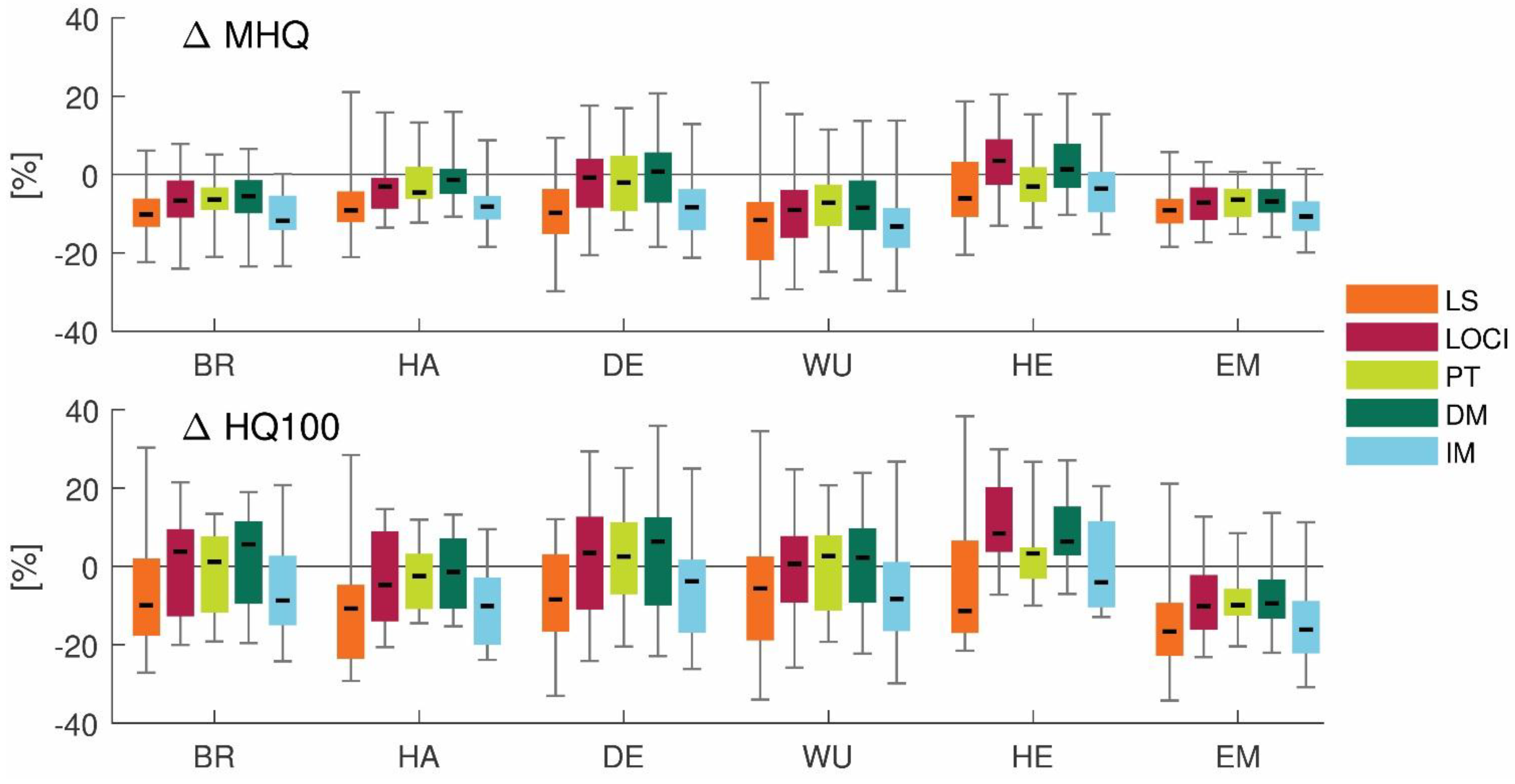
4.4. Impact of Bias Correction on the Future Projections of Precipitation and Discharge

Figure 5 shows the climate change signals for P95d3 and for MHQ for bias-corrected and non-corrected climate scenario data. In terms of P95d3, an increase was simulated by all climate scenarios and both RCP scenarios. These climate change signals are generally higher for RCP8.5 than for RCP4.5 and mostly they are higher for the bias-corrected data. The deviations between the signals of corrected and non-corrected data are higher for the BC methods power transformation, distribution mapping or LOCI than for linear scaling and the ISI-MIP approach.
In terms of MHQ, the climate change signals projected by non-corrected data show on average only small changes for RCP4.5 and an increase of ca. 10% for RCP8.5. BC mostly leads to higher change signals in case the signal of non-corrected data was positive. In case of a negative signal obtained by non-corrected data, the BC led to either a smaller negative or even positive signal. Typically, for MHQ the deviations of the signals among the different BC methods are smaller than the difference between the signals of one BC method and non-corrected data for one climate scenario and one RCP scenario.
The deviations in climate change signals are higher for MHQ than for P95d3.

4.5. Evaluation of Climate Scenarios

The results for the evaluation of BC methods for both objectives, the agreement of Qhist,bc with Qref and the maintenance of the climate change signal obtained by non-corrected data Porig by the corrected data Pbc are shown in Figure 6.
The methods do not show great differences regarding monthly mean discharge, MMQD, but there are differences regarding the performance for the simulated MHQ. Power transformation, distribution mapping and LOCI perform better than linear scaling and the ISI-MIP approach.
For the evaluation of MMPSigD, the methods delta change, linear scaling and ISI-MIP are not included, because of the perfect agreement with the signal obtained from non-bias-corrected data (see Section 3.5). LOCI performs better than distribution mapping and power transformation. For P95d3SidD, the performance of the ISI-MIP approach and linear scaling is significantly better than the other methods, whereas delta change shows a much lower performance.

5. Discussion and Conclusions

The comparison of observed and simulated climate variables showed a significant bias in climate scenario data. When applying this data to hydrological models, significant impacts on hydrological parameters are the consequence. Substantial differences in the discharge volume indicate fundamentally changed hydrological processes, e.g., an altered ratio of discharge and infiltration due to much higher water saturation of the soil or a significantly higher groundwater recharge. Therefore, applying bias-correction on climate model data prior to the use as input data for hydrological models seems necessary as it leads to simulations of hydrological processes that correspond much better to observed conditions.
The sensitivity analysis showed that deviation in precipitation of the climate scenario data are by far the most critical factor with respect to the simulated discharge. Therefore, the variable precipitation should be bias-corrected for a plausible simulation of discharge. Besides, temperature is often bias-corrected in hydrological climate impact studies. Our findings moreover suggest investigating biases in all climate variables that are used as input for the hydrological model as they can cause substantial deviations in discharge (mean flows and high flows) as well.
Higher climate change signals for high precipitation parameters were calculated for bias-corrected climate scenario data than for non-corrected data. The deviations for the climate change signals for high flow parameters are even larger than those for high precipitation parameters when using the corrected/non-corrected climate scenario data as input for the hydrological model. In most cases when the signal for the high flow parameter MHQ obtained by non-corrected climate scenario data was positive, the application of BC led to higher signals. In case the signal with non-corrected climate scenario data was negative, the signal with bias-corrected data was lower or even positive.
It could be argued that in climate change studies the most relevant result is the climate change signal and not absolute values, e.g., of discharge. However, it should be considered that signals that are based on simulations are supposed to represent the process dynamics of a certain region. If these processes significantly differ from realistic conditions, because of high deviations in input data, the magnitude of climate change signals obtained by these simulations have to be critically questioned. Therefore, BC should be applied when climate scenario data significantly differ from observations.
The evaluation results also showed that no BC method is clearly better than the others in terms of all evaluated criteria. While power transformation, LOCI and distribution mapping led to a more sophisticated representation of high flows during the reference period, linear scaling and ISI-MIP were better capable of maintaining the projected changes of the non-corrected data in terms of monthly precipitation and high precipitation values.
An assumption of BC in general is that the deviations found for the reference period remain constant over time. This can be doubted, as it was shown, for example by [14], that BC procedure may be sensitive to the choice of the reference period. Lafon, T. et al. [14] found less complex methods to be more robust and less vulnerable to over-tuning. From this study covering the historic period it cannot be concluded that the less complex methods lead to more realistic corrections of the simulations of future climate as variations between slightly modified reference periods can be expected to be smaller than the variations between future climate, especially at the end of the 21st century, and the reference period. Due to the projected changes in climate variables, the reliability of the calibrated BC procedure for all BC methods may decline in the course of the century.
When investigating climate change impacts on hydrological parameters on a regional scale, the additional source of uncertainty of BC to the entire model chain uncertainty should not be neglected. In case only one BC method can be applied, the performance of the selected method related to the study objective should be evaluated for the study area in advance.

Author Contributions

Conceptualization V.W. and P.K.; methodology V.W.; software V.W. and P.K.; validation, P.K.; formal analysis V.W. and P.K.; investigation V.W.; resources V.W.; data curation V.W.; writing—original draft preparation, V.W.; writing—review and editing P.K. and G.M.; visualization V.W.; supervision G.M.; project administration P.K.; funding acquisition G.M.

Funding

This research received no external funding.

Acknowledgments

We acknowledge the World Climate Research Programme’s Working Group on Regional Climate, and the Working Group on Coupled Modelling, former coordinating body of CORDEX and responsible panel for CMIP5. We also thank the climate modelling groups (listed in Table 1 of this paper) for producing and making available their model output. We also acknowledge the Earth System Grid Federation infrastructure an international effort led by the U.S. Department of Energy’s Program for Climate Model Diagnosis and Intercomparison, the European Network for Earth System Modelling and other partners in the Global Organisation for Earth System Science Portals (GO-ESSP).

Conflicts of Interest

The authors declare no conflict of interest.

References

  1. IPCC. Climate Change 2014: Synthesis Report. Contribution of Working Groups I, II and III to the Fifth Assessment Report of the Intergovernmental Panel on Climate Change; Core Writing Team, Pachaur, R.K., Meyer, L.A., Eds.; Intergovernmental Panel on Climate Change: Geneva, Switzerland, 2014; ISBN 978-92-9169-143-2. [Google Scholar]
  2. Pendergrass, A.G.; Hartmann, D.L. Changes in the Distribution of Rain Frequency and Intensity in Response to Global Warming. J. Clim. 2014, 27, 8372–8383. [Google Scholar] [CrossRef]
  3. Dai, A.; Rasmussen, R.M.; Liu, C.; Ikeda, K.; Prein, A.F. A new mechanism for warm-season precipitation response to global warming based on convection-permitting simulations. Clim. Dyn. 2017, 321, 1481. [Google Scholar] [CrossRef]
  4. Prein, A.F.; Rasmussen, R.M.; Ikeda, K.; Liu, C.; Clark, M.P.; Holland, G.J. The future intensification of hourly precipitation extremes. Nat. Clim. Change 2017, 7, 48–52. [Google Scholar] [CrossRef]
  5. Alfieri, L.; Dottori, F.; Betts, R.; Salamon, P.; Feyen, L. Multi-Model Projections of River Flood Risk in Europe under Global Warming. Climate 2018, 6, 6. [Google Scholar] [CrossRef]
  6. Hattermann, F.F.; Kundzewicz, Z.W.; Huang, S.; Vetter, T.; Gerstengarbe, F.-W.; Werner, P. Climatological drivers of changes in flood hazard in Germany. Acta Geophys. 2013, 61, 463–477. [Google Scholar] [CrossRef]
  7. NLWKN. Globaler Klimawandel—Wasserwirtschaftliche Folgen für das Binnenland. Gesamtbericht des Projektes KliBiW Themenbereich Hochwasser; NLWKN: Norden, Germany, 2017. [Google Scholar]
  8. Ehret, U.; Zehe, E.; Wulfmeyer, V.; Warrach-Sagi, K.; Liebert, J. HESS Opinions “Should we apply bias correction to global and regional climate model data?”. Hydrol. Earth Syst. Sci. 2012, 16, 3391–3404. [Google Scholar] [CrossRef]
  9. Rauscher, S.A.; Coppola, E.; Piani, C.; Giorgi, F. Resolution effects on regional climate model simulations of seasonal precipitation over Europe. Clim. Dyn. 2010, 35, 685–711. [Google Scholar] [CrossRef]
  10. Piani, C.; Weedon, G.P.; Best, M.; Gomes, S.M.; Viterbo, P.; Hagemann, S.; Haerter, J.O. Statistical bias correction of global simulated daily precipitation and temperature for the application of hydrological models. J. Hydrol. 2010, 395, 199–215. [Google Scholar] [CrossRef]
  11. Jakob Themeßl, M.; Gobiet, A.; Leuprecht, A. Empirical-statistical downscaling and error correction of daily precipitation from regional climate models. Int. J. Climatol. 2011, 31, 1530–1544. [Google Scholar] [CrossRef]
  12. Teutschbein, C.; Seibert, J. Bias correction of regional climate model simulations for hydrological climate-change impact studies: Review and evaluation of different methods. J. Hydrol. 2012, 456–457, 12–29. [Google Scholar] [CrossRef]
  13. NLWKN. Globaler Klimawandel—Wasserwirtschaftliche Folgen für das Binnenland. Niedrigwasser; NLWKN: Norden, Germany, 2014. [Google Scholar]
  14. Lafon, T.; Dadson, S.; Buys, G.; Prudhomme, C. Bias correction of daily precipitation simulated by a regional climate model: A comparison of methods. Int. J. Climatol. 2013, 33, 1367–1381. [Google Scholar] [CrossRef]
  15. Huang, S.; Krysanova, V.; Hattermann, F.F. Does bias correction increase reliability of flood projections under climate change? A case study of large rivers in Germany. Int. J. Climatol. 2014, 34, 3780–3800. [Google Scholar] [CrossRef]
  16. Teng, J.; Potter, N.J.; Chiew, F.H.S.; Zhang, L.; Wang, B.; Vaze, J.; Evans, J.P. How does bias correction of regional climate model precipitation affect modelled runoff? Hydrol. Earth Syst. Sci. 2015, 19, 711–728. [Google Scholar] [CrossRef] [Green Version]
  17. Jacob, D.; Petersen, J.; Eggert, B.; Alias, A.; Christensen, O.B.; Bouwer, L.M.; Braun, A.; Colette, A.; Déqué, M.; Georgievski, G.; et al. EURO-CORDEX: New high-resolution climate change projections for European impact research. Reg. Environ. Change 2014, 14, 563–578. [Google Scholar] [CrossRef]
  18. Moss, R.H.; Edmonds, J.A.; Hibbard, K.A.; Manning, M.R.; Rose, S.K.; van Vuuren, D.P.; Carter, T.R.; Emori, S.; Kainuma, M.; Kram, T.; et al. The next generation of scenarios for climate change research and assessment. Nature 2010, 463, 747–756. [Google Scholar] [CrossRef] [PubMed]
  19. Bolton, D. The Computation of Equivalent Potential Temperature. Mon. Wea. Rev. 1980, 108, 1046–1053. [Google Scholar] [CrossRef] [Green Version]
  20. Smiatek, G.; Kunstmann, H.; Senatore, A. EURO-CORDEX regional climate model analysis for the Greater Alpine Region: Performance and expected future change. J. Geophys. Res. Atmos. 2016, 121, 7710–7728. [Google Scholar] [CrossRef]
  21. Schmidli, J.; Frei, C.; Vidale, P.L. Downscaling from GCM precipitation: A benchmark for dynamical and statistical downscaling methods. Int. J. Climatol. 2006, 26, 679–689. [Google Scholar] [CrossRef]
  22. Riedel, G.; Lichtenberg, T. Panta Rhei User Manual; Department of Hydrology, Water Management and Water Protection of TU Braunschweig: Braunschweig, Germany; Institut für Wassermanagement IfW: Braunschweig, Germany, 2017. [Google Scholar]
  23. Kreye, P. Mesoskalige Bodenwasserhaushaltsllierung mit Nutzung von Grundwassermessungen und satellitenbasierten Bodenfeuchtedaten. Ph.D. Thesis, University of Braunschweig, Braunschweig, Germany, 2015. [Google Scholar]
  24. Meon, G.; Pätsch, M.; van Phuoc, N.; Hong Quan, N. EWATEC-COAST: Technologies for Environmental and Water Protection of Coastal Regions in Vietnam. Contribution to 4th International Conference for Environment and Natural Resources – ICENR, Ho-Chi-Minh City, Vietnam, 17–18 June 2014; Cuvillier: Göttingen, Germany, 2014. [Google Scholar]
  25. Riedel, G.; Anhalt, M.; Meyer, S.; Weigl, E.; Meon, G. Erfahrung mit Radarprodukten bei der operationellen Hochwasservorhersage in Niedersachsen. KW - Korrespondenz Wasserwirtschaft 2017, 11, 664–671. [Google Scholar]
  26. Gelleszun, M.; Kreye, P.; Meon, G. Representative parameter estimation for hydrological models using a lexicographic calibration strategy. J. Hydrol. 2017, 553, 722–734. [Google Scholar] [CrossRef]
  27. Nash, J.E.; Sutcliffe, J.V. River flow forecasting through conceptual models part I—A discussion of principles. J. Hydrol. 1970, 10, 282–290. [Google Scholar] [CrossRef]
  28. Leander, R.; Buishand, T.A. Resampling of regional climate model output for the simulation of extreme river flows. J. Hydrol. 2007, 332, 487–496. [Google Scholar] [CrossRef]
  29. Teutschbein, C.; Seibert, J. Is bias correction of regional climate model (RCM) simulations possible for non-stationary conditions? Hydrol. Earth Syst. Sci. 2013, 17, 5061–5077. [Google Scholar] [CrossRef] [Green Version]
  30. Piani, C.; Haerter, J.O.; Coppola, E. Statistical bias correction for daily precipitation in regional climate models over Europe. Theor. Appl. Climatol. 2010, 99, 187–192. [Google Scholar] [CrossRef]
  31. Hempel, S.; Frieler, K.; Warszawski, L.; Schewe, J.; Piontek, F. A trend-preserving bias correction—The ISI-MIP approach. Earth Syst. Dynam. 2013, 4, 219–236. [Google Scholar] [CrossRef]
  32. Räty, O.; Räisänen, J.; Ylhäisi, J.S. Evaluation of delta change and bias correction methods for future daily precipitation: Intermodel cross-validation using ENSEMBLES simulations. Clim. Dyn. 2014, 42, 2287–2303. [Google Scholar] [CrossRef]
  33. Cannon, A.J.; Sobie, S.R.; Murdock, T.Q. Bias Correction of GCM Precipitation by Quantile Mapping: How Well Do Methods Preserve Changes in Quantiles and Extremes? J. Clim. 2015, 28, 6938–6959. [Google Scholar] [CrossRef]
  34. O’Gorman, P.A.; Muller, C.J. How closely do changes in surface and column water vapor follow Clausius–Clapeyron scaling in climate change simulations? Environ. Res. Lett. 2010, 5, 25207. [Google Scholar] [CrossRef]
  35. Kling, H.; Fuchs, M.; Paulin, M. Runoff conditions in the upper Danube basin under an ensemble of climate change scenarios. J. Hydrol. 2012, 424–425, 264–277. [Google Scholar] [CrossRef]
Figure 1. Grid cell centers of the original Coordinated Downscaling Experiment for Europe (CORDEX) grid, the interpolated 10 × 10 km grid and the location of the six catchments.
Hydrology 06 00046 g001
Figure 2. Mean values of climatological and hydrological variables for the catchment Wunstorf for the historical period 1971–2000 for all climate scenarios and observations (Xobs). For discharge, the results of the hydrological modeling with climate scenario data and observational data (Qref) are shown.
Hydrology 06 00046 g002
Figure 3. Result of the sensitivity analysis for climate variables. The bars represent the deviations in MQ and MHQ for the simulation runs with altered climate variables (Wind = wind speed, Hum = relative humidity, Rad = global radiation, T = temperature and P = precipitation) according to the three sensitivity levels compared to Qref.
Hydrology 06 00046 g003
Figure 4. Percentage deviations for MHQ and HQ100 between the simulations with bias corrected climate scenario data and observed climate data for the historical period 1971–2000 for six catchments (Bramsche-BR, Harxbuettel-HA, Derneburg-DE, Wunstorf-WU, Hellwege-HE and Emlichheim-EM) applying different bias-correction (BC) methods (linear scaling (LS), local intensity scaling (LOCI), power transformation (PT), distribution mapping (DM) and Inter-Sectoral Impact-Model Intercomparison Project (ISI-MIP) approach (IM)) for precipitation and linear scaling for the other climate variables.
Hydrology 06 00046 g004
Figure 5. Climate change signals for P95d3 and MHQ for 17 climate scenarios for the non-corrected climate scenario data and differently bias-corrected data as mean of the grid cells for the whole area (P95d3) or as weighted mean by catchment size (MHQ) for the period 2070–2099 compared to the historical period 1971–2000. The correction methods are: linear scaling (LS), power transformation (PT), distribution mapping (DM), LOCI and the ISI-MIP approach (IM).
Hydrology 06 00046 g005
Figure 6. Performance of different bias correction methods in terms of (upper charts): MHQ and monthly mean values of discharge and (lower charts): the climate change signals for the 95% percentile of 3-day precipitation sum, P95d3SigD, and for the monthly mean precipitation MMPSigD. Evaluated BC methods: LS = linear scaling, PT = power transformation, DM = distribution mapping, IM = the ISI-MIP approach, DC = delta change and LOCI.
Hydrology 06 00046 g006
Table 1. General circulation model/regional climate model (GCM/RCM) combination matrix. S7 and S8, as well as S16 and S17 are combinations of the same GCM and RCM. They are different in terms of the GCM run with which the RCM was driven.
Institution →SMHIIPSL-INERISKNMIDMICLMcomMPI-CSC
GCM ↓ RCM →RCA4WRF331FRACMO22EHIRHAM5CCLMREMO2009
CNRM_CM5S1 S12
EC-EarthS2 S7, S8S10S13
IPSL-CM5A-MRS3S6
HadGEM2-ESS4 S9 S14
MPI-ESM-LRS5 S15S16, S17
NorESM1-M S11
Table 2. Deviations of climate variables and simulated discharge parameters between climate scenario data and observational data for the period 1971–2000. Climate variables: temperature (T), precipitation (P), 95% percentile of precipitation/3-day precipitation sum (P95/P95d3), number of wet days >1 mm (WD1), wind Speed (Wind), global radiation (Rad) and relative humidity (Hum); hydrological parameters: mean discharge (MQ) and mean annual peak flow (MHQ).
Scenario∆T [°C]∆P [%]∆P95 [%]∆P95d3 [%]∆WD1 [%]∆Wind [%]∆Rad [%]∆Hum [%]∆MQ [%]∆MHQ [%]
S1−1.338.13.28.133.094.131.36.867.439.9
S2−1.640.64.210.734.5105.829.36.174.452.5
S3−1.454.7−1.45.252.1112.222.57.3122.972.5
S4−0.329.90.65.825.7100.830.74.860.040.4
S5−0.256.77.613.342.9103.224.58.7110.265.6
S6−1.130.5−0.31.428.1143.236.40.852.467.1
S7−2.110.3−14.2−9.820.1122.012.52.824.833.0
S8−1.610.0−15.5−10.520.0123.614.22.026.626.3
S9−1.012.0−10.0−7.418.0122.515.12.336.944.9
S10−1.122.31.34.418.8101.73.51.656.363.8
S110.048.56.411.238.1106.4−2.53.7121.4105.1
S12−1.43.6−9.0−10.410.795.713.72.711.516.1
S13−1.4−3.9−7.9−9.33.4107.014.51.0−4.63.7
S14−0.3−14.6−12.6−13.7−6.2105.319.2−2.8−3.018.9
S15−0.622.6−5.6−5.124.5112.34.16.852.618.4
S160.320.3−5.4−2.022.693.40.94.434.528.4
S170.622.3−6.9−1.625.294.90.84.244.338.5
Mean−0.823.8−3.9−0.624.2108.515.93.752.343.2

