Abstract
Construction of flow duration curves (FDCs) is a challenge for hydrologists as most streams and rivers worldwide are ungauged. Regionalization methods are commonly followed to solve the problem of discharge data scarcity by transforming hydrological information from gauged basins to ungauged basins. As a consequence, regionalization-based FDC predictions are not very reliable where discharge data are scarce quantitatively and/or qualitatively. In such a scenario, it is perhaps more meaningful to use a calibration-free rainfall‒runoff model that can exploit easily available meteorological information to predict FDCs in ungauged basins. This hypothesis is tested in this study by comparing a well-known regionalization-based model, the inverse distance weighting (IDW) model, with the recently proposed calibration-free dynamic Budyko model (DB) in a region where discharge observations are not only insufficient quantitatively but also show apparent signs of observational errors. The DB model markedly outperformed the IDW model in the study region. Furthermore, the IDW model’s performance sharply declined when we randomly removed discharge gauging stations to test the model in a variety of data availability scenarios. The analysis here also throws some light on how errors in observational datasets and drainage area influence model performance and thus provides a better picture of the relative strengths of the two models. Overall, the results of this study support the notion that a calibration-free rainfall‒runoff model can be chosen to predict FDCs in discharge data-scarce regions. On a philosophical note, our study highlights the importance of process understanding for the development of meaningful hydrological models.
1. Introduction
Sustainable water resources management and the designing of numerous hydraulic infrastructure schemes require flow duration curves (FDCs), which can be obtained using historical streamflow information. FDC encodes complex hydrological information in terms of a simple numerical expression, the complement of cumulative probability distribution of streamflow [1,2]. However, unavailability of discharge data is a major challenge for hydrologists as most rivers and streams in the world are either ungauged or poorly gauged [3,4,5,6]. Therefore, hydrologists have developed several regionalization methods to predict FDCs in ungauged basins by transferring information from gauged basins to ungauged basins [6,7,8,9,10,11,12,13,14,15]. Typically, FDCs are predicted in ungauged basins by regionalizing flow quantiles using discharge data from ‘hydrologically similar’ gauged basins [16,17,18,19,20]. The reasoning is that if two basins possess similar physical and climatological characteristics, they are likely to exhibit a similar hydrological response.
Construction of FDC in an ungauged basin with the help of a regionalization-based FDC model thus requires discharge data from hydrologically similar gauged basins [6,8,13]. Since there is no objective way to quantify how similar two basins are, a regionalization-based FDC model’s performance is expected to be sensitive to the availability of discharge data from gauged basins [21]. Conversely, we cannot reliably predict FDC in the ungauged basin if the gauged basins are not adequately similar to it. This problem is more likely to occur in a region with low streamflow gauging station density [22,23,24]. We need discharge data from a large number of gauged basins to predict FDC in an ungauged basin, and the available discharge data must be accurate [25]. However, to our knowledge, there are no clear guidelines in the hydrologic literature on how to predict FDCs in ungauged basins when discharge data (from gauged basins) are not only quantitatively inadequate but also qualitatively poor. Furthermore, the FDC predicted for an ungauged basin with the help of a regionalization-based FDC model will not be useful for a future time period if the local climate undergoes significant changes [23].
In contrast to the situation of discharge data scarcity in most parts of the world, it is becoming easier to obtain meteorological information everywhere, mainly due to advancements in satellite remote sensing and numerical weather forecasting [26,27,28,29,30,31]. Thus to address the issue of discharge data scarcity, many hydrologists have suggested the use of process-based models that can effectively exploit easily available meteorological data to predict FDCs for ungauged basins. One possibility is to employ a process-based rainfall‒runoff model to obtain discharge time series for ungauged basins using meteorological data and then construct FDCs [22]. However, traditional rainfall‒runoff models have multiple free parameters. They can be used for prediction in ungauged basins only after regionalizing the model parameters using discharge data from gauged basins [32,33,34,35], which implies that FDC prediction in ungauged basins with the help of a rainfall‒runoff model with regionalized parameters may not be very reliable in discharge data-scarce regions.
One way to address the above issue is to develop a rainfall‒runoff model that does not even have a single free parameter, i.e., an inherently calibration-free rainfall‒runoff model. Such a model will not be affected by discharge data scarcity as it will not need discharge data in the first place. In an ideal world, we would expect every hydrological model to be purely physics-based and to deliver accurate predictions without any calibration (e.g., [21]). In reality, very little research has been devoted towards developing calibration-free hydrological models as it is generally believed that no hydrological model can perform reasonably well without calibration. In this study, we argue that a calibration-free rainfall-runoff model can be used to predict FDC in regions where observed discharge data are inadequate both quantitatively and qualitatively. In particular, we, for the first time, use the recently developed calibration-free dynamic Budyko model to predict FDCs in totally ungauged basins. To assess the usefulness of the calibration-free model, we compare it with a well-known regionalization-based FDC model in south India. Furthermore, we perform a detailed analysis to understand how errors in input data and drainage area affect the performance of the two models. Our aim is to objectively assess the relative merits and demerits of the two models. In the next section, we provide details about the methods that are employed for this study.
2. Data and the FDC Models
2.1. The Study Basins and Preliminary Data Processing
The numerical experiments in this study are carried out using discharge time series data from Central Water Commission (CWC) gauging stations that are situated in the Krishna and the Godavari river basins, the two main river basins in south India. Large basins (basins with drainage area greater than 21,000 km2) are excluded as the dynamic Budyko model does not account for flow routing in channel networks. In total, 50 basins are selected for the preliminary analysis. For each basin five years of continuous discharge observations (in mm/day) are considered for model evaluation. The study basins have drainage areas ranging between 550 km2 and 20,967 km2. Gridded daily mean rainfall (from 1901 to 2015 at 0.25-degree resolution) and temperature (maximum, minimum, and average temperatures from 1951 to 2014 at 0.5-degree resolution) datasets are obtained from the Indian Meteorological Department, IMD (http://www.imdpune.gov.in/). The gridded datasets were prepared by IMD using ground-based observations and following an interpolation technique [36]. We use the temperature time series to compute potential evapotranspiration at subgrid scale following the method proposed by Hargreaves and Samani [37]. Then, for each basin, we obtain rainfall and potential evapotranspiration time series (in mm/day) by performing spatial averaging of the gridded time series data.
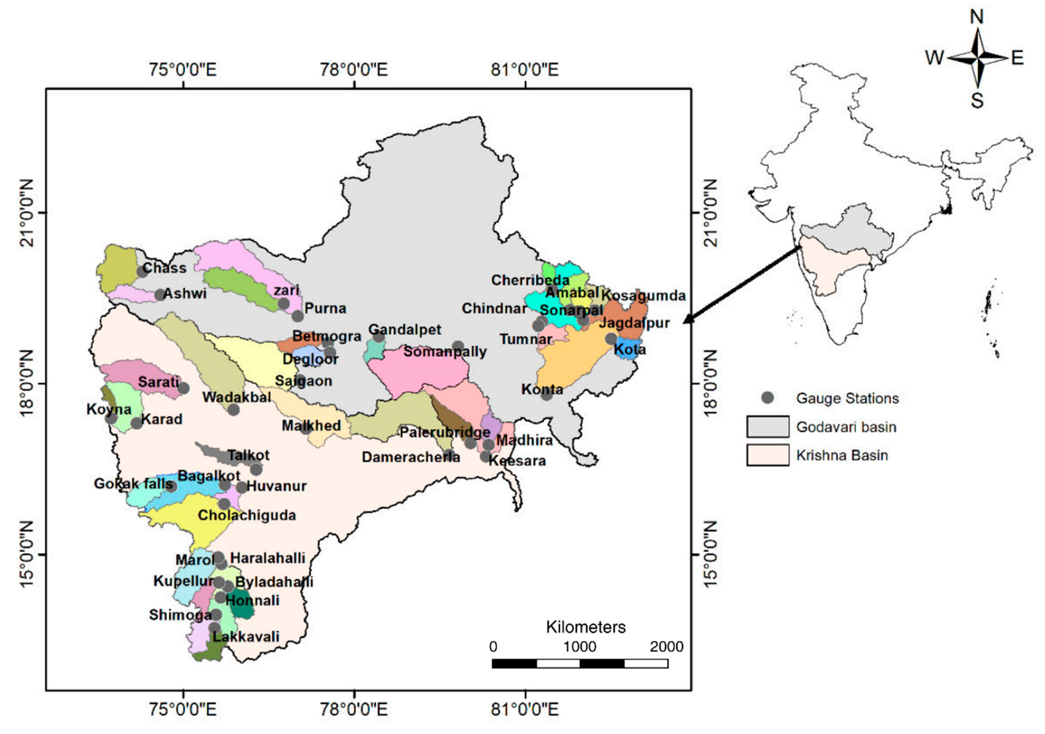
It should be noted that hydrological measurements are often associated with significant errors [38,39,40,41,42,43,44]. Often simple criteria are followed to discard erroneous data. In this study, we discarded basins with a runoff ratio greater than 1 because it is highly unlikely for a basin to have a mean runoff that is greater than the mean rainfall, particularly in south India, where mean potential evapotranspiration is quite high (Table S1). We also discarded basins with a runoff ratio less than 0.1 as it is known that basins with a very low runoff ratio are likely to be associated with significant observational errors [45]. The remaining basins (40 in total, see Figure 1) were then considered for FDC model evaluation.

Figure 1.
Map showing the locations of the 40 study basins considered for evaluating the two FDC models.
First, the observed discharge time series data were considered for constructing FDCs following Weibull’s plotting position formula [46]. For a study basin, say the th basin, discharge quantiles are obtained by simply ranking the observed discharge () values. The total number of discharge quantiles () is thus equal to the total number of data point in the discharge time series. Note that here always equals since we considered five years of discharge data for every basin. The probability (in percentage) of a randomly chosen discharge value exceeding the th observed discharge quantile ()) of the th basin is computed here following Weibull’s plotting position formula:
The observed flow duration curve for the basin is constructed by computing the exceedance probability of each discharge quantile following Equation (1) and then plotting the vs. curve. The above steps are followed to obtain observed FDCs for all the 40 study basins (Figure 2).
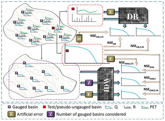
Figure 2.
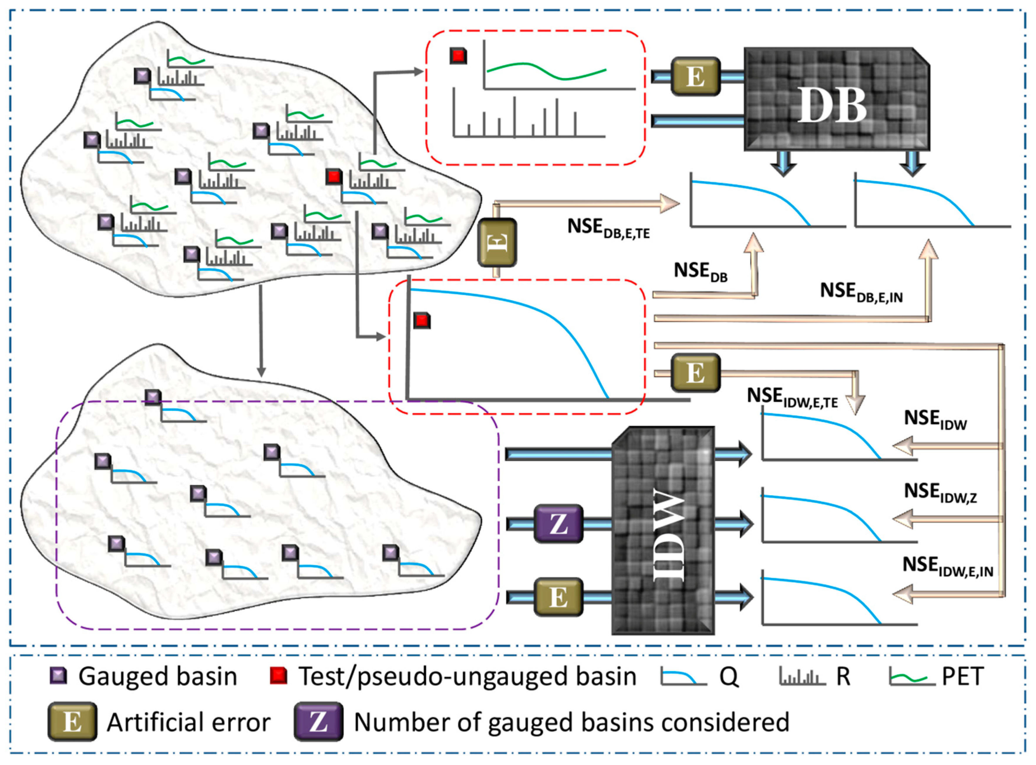
Schematic diagram depicting the model evaluation exercise performed in this study. Let us consider a hypothetical case of a region with data from basins to evaluate the two FDC models (DB and IDW). Each basin has observed discharge time series from which flow duration curve (FDC) is obtained. Also, each basin has rainfall and PET time series data. Consider one of the basins (say the th basin) as the test/pseudo-ungauged basin whose FDC is now the ‘test data’ (see the legend). Its R and PET time series are now the ‘input data’ for the DB model. For the IDW model, however, FDCs from the remaining basins are considered as the input dataset. The FDC from the test (th) basin is then compared separately with the FDCs generated by the two models and and are computed for the test basin. We also test the IDW model in different discharge data availability scenarios by using FDCs only from number of randomly selected basins (from the input basins) and compute for the test basin. Furthermore, we analyse how the two models are sensitive to errors in the observed data by adding artificial error () into the input data (the rainfall and PET time series in case of the DB model and the FDCs from the ‘gauged basins’ for the IDW model) as well as the test data (the FDC of the test basin) and report the s. All the above steps are repeated considering every other study basin as the test basin. Note that in our study.
2.2. Two Models for Predicting FDCs in Ungauged Basins
The two models used in this study for simulating FDCs are: the dynamic Budyko (DB) model [47] and the inverse distance weighted (IDW) model [9,13,46]. The DB model is a process-based dynamic rainfall‒runoff model that uses rainfall and potential evapotranspiration data as inputs to simulate discharge (Figure 2). Since the model does not have a single free parameter, it can be applied in a completely ungauged region to construct FDCs using only meteorological data. On the other hand, the IDW model is a regionalization-based statistical FDC model. To apply it for predicting FDC in an ungauged basin, one needs to have adequate discharge data from hydrological similar basins. In the following subsections, we provide a brief overview of the structures of the two models.
2.2.1. The DB Model
The model mainly consists of two conceptual zones that are responsible for partitioning rainfall (R) and solar energy, expressed as potential evapotranspiration (PET). The model adopts a two-stage partitioning scheme. In stage one rainfall needs to satisfy evapotranspiration demand of the basin, which is equal to the PET at that time. If R > PET, the remaining water (W) enters into stage two. Similarly, if R < PET, the remaining solar energy (H) enters into stage two. The interaction between W and H determines the partitioning of W into effective rainfall (ER), the fraction of W that eventually transforms into streamflow, and rainfall loss (RL), the fraction of rainfall that eventually exit the basin as evapotranspiration. It is hypothesized that at any point of time the partitioning of W into ER and RL is primarily determined by the instantaneous dryness-index () of the basin [47]:
is the original Budyko function, which, for a given instantaneous dryness-index, can be expressed as . It is assumed that is a function of antecedent W and H inputs. The effect of input W or H on basin dryness decreases with time following an empirically derived ‘universal’ decay function [47], where is the effect of at time . The decay function is the main building block of the model. The model essentially assumes that basins across geographical and climatic regions can be characterized by a single decay function. This is akin to saying all the real basins are similar to each other in the way they transform rainfall into streamflow. Although a detailed discussion of this subject is beyond the scope of this article, analogous arguments can be found elsewhere in the hydrologic literature (e.g., [48,49]).
One can now define functional W (FW) and functional H (FH) affecting the dryness state of the basin at a given time: and , where is a dummy variable. is the number of days for which the effect of and last, and its value is fixed at 365 [47]. Similar to the definition of the dryness index, the instantaneous dryness index is then defined as: . Finally, discharge at any point of time is computed considering the same decay function [47]:
The model is used to simulate discharge at a daily time step by discretizing the equations (for details, see [47]). The DB model-based FDC for the th study basin can then be easily constructed by first obtaining the discharge quantiles (s) and then plotting vs. following Equation (1) (see Figure 2). FDCs can be obtained similarly for all the other 39 study basins.
2.2.2. The IDW Model
The IDW model is a frequently used for predicting FDCs in ungauged basins [9,13,50,51,52]. Its main appeal is its simplicity [50]. Here we follow a leave-one-out-type cross-validation approach to predict FDC for each of the 40 () study basins by employing the IDW model [53]. The entire method is discussed in the following steps. Observed flow quantiles (s) of the th basin are kept aside as test data for evaluating the model. Observed discharge quantiles from the remaining 39 ( basins are considered as ‘input data’, and the IDW model is employed to predict discharge quantiles for the th basin:
where is the geographical distance between the outlets of the th basin and the th basin. Equation (4) essentially suggests that hydrological similarity weakens with geographical distance [51]. The above step was repeated for all the values of . The IDW model-based FDC for the th basin is constructed by plotting vs. following Equation (1) (Figure 2). All the above steps were then repeated for each of the remaining 39 study basins.
2.3. Model Performance Evaluation
We evaluated the two models by comparing modelled and observed/test discharge quantiles in terms of NSE [54]. For the th basin, the NSEs were computed as: and , where is the mean of the observed discharge quantiles of the basin (Figure 2). NSE values were similarly computed for the remaining 39 study basins. We then focussed on studying how sensitive the models are to discharge data scarcity and to observational errors.
2.3.1. How Sensitive Is the IDW Model to Discharge Data Scarcity?
Since the DB model requires only meteorological information for predicting FDC for any basin, its performance is totally insensitive to discharge data availability. On the other hand, the IDW model requires input (discharge) data from gauged basins to predict FDC for an ungauged basin, and thus its performance is expected to be sensitive to discharge data availability [22,23]. To test the IDW model’s performance in different data availability situations, we systematically remove study basins from the input database. The analysis is performed as described in the following steps. For the th selected basin, discharge quantiles are again kept aside as test data. From the remaining 39 basins, we randomly select number of basins and use their discharge quantiles as input data and predict discharge quantiles for the test (th) basin using the IDW model as discussed in Section 2.2.2 (see also Figure 2). We then compare the observed discharge quantiles (test data) and the discharge quantiles predicted by the IDW model using data from the basins in terms NSE. To make our analysis robust, we repeated the above steps 10 times (i.e., 10 random groups each with number of randomly selected basins) and considered the mean of the NSEs as the representative NSE () for the test basin. We performed this experiment for the following values of : 36, 28, 20, and 12. Then, for each of the remaining 39 study basins, all the above steps were repeated and for each was obtained.
2.3.2. How Do Errors in Data Influence Model Performance?
NSE ranges between and ; the higher its value, the better, we consider, is the model performance. However, how errors in input data as well as in test data influence model performance is less frequently discussed [55,56,57,58,59]. This discussion is relevant here, particularly because the two models require entirely different input datasets. Here, we investigated the effect of data errors on model performance by artificially introducing errors in both input data and test data (see Figure 2). Assuming that the percentage errors in any of the time series here constitute uniformly distributed random numbers between two given numbers, which is represented by the function (each time is recalled, it returns a random number between the two numbers). If we introduce to a certain time series (), the modified value of the th element in the time series () will be equal to .
In this study we considered three types of error distributions: unskewed, positively skewed, and negatively skewed. We selected two unskewed type uniform error distributions with ranges from −40 to 40 () and from −80 to 80 (). Similarly, we chose two positively skewed uniform distributions with ranges from 0 to 40 () and from 0 to 80 () and two negatively skewed distributions with ranges from −40 to 0 () and from −80 to 0 (). We considered all the six error distributions and investigated how errors in input data influence model performance. Thus for the DB model, we applied each of the six error distributions separately to the rainfall and PET time series data (input data) and recalculated NSE () for the test basin. In the case of the IDW model, however, the analysis was quite different. For each selected basin the test discharge quantiles were left untouched, while errors were introduced to the input discharge quantiles from the reaming 39 study basins. We recalculated NSE () for the test basin, considering error in the input dataset separately for each of the six error distributions. We then focussed our attention on investigating the impact of errors in test data on model performance. We thus recalculated NSE by applying each of the six error distributions to the test basin’s observed discharge quantiles separately for both the DB model () and the IDW model ().
3. Results and Discussion
3.1. Model Performance Comparison
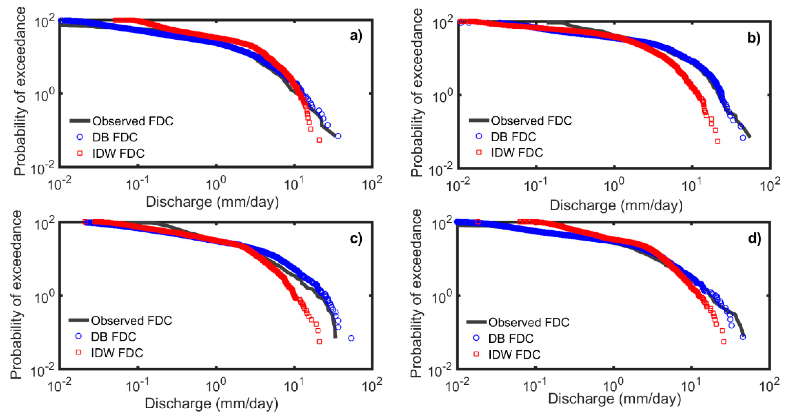
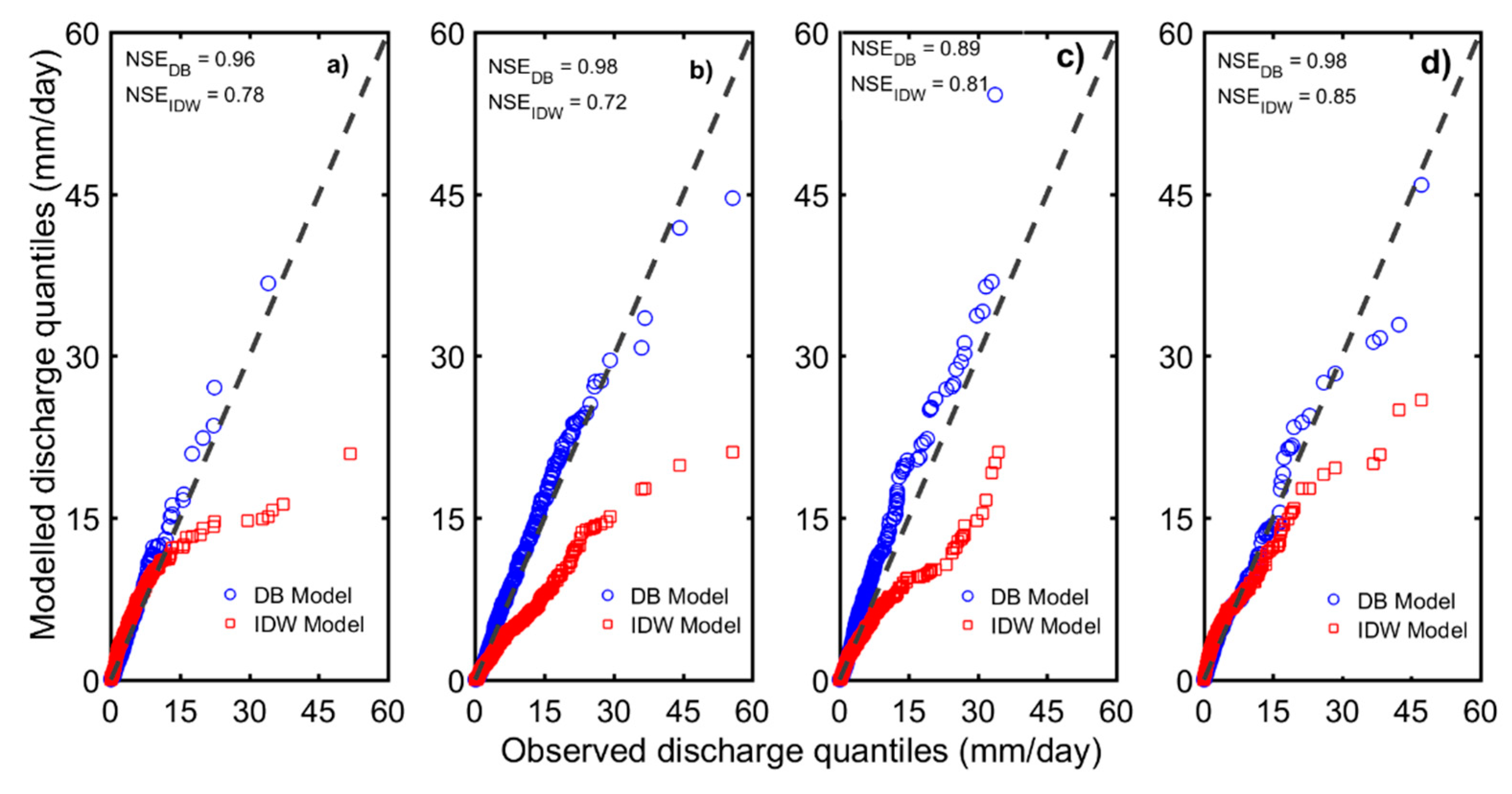
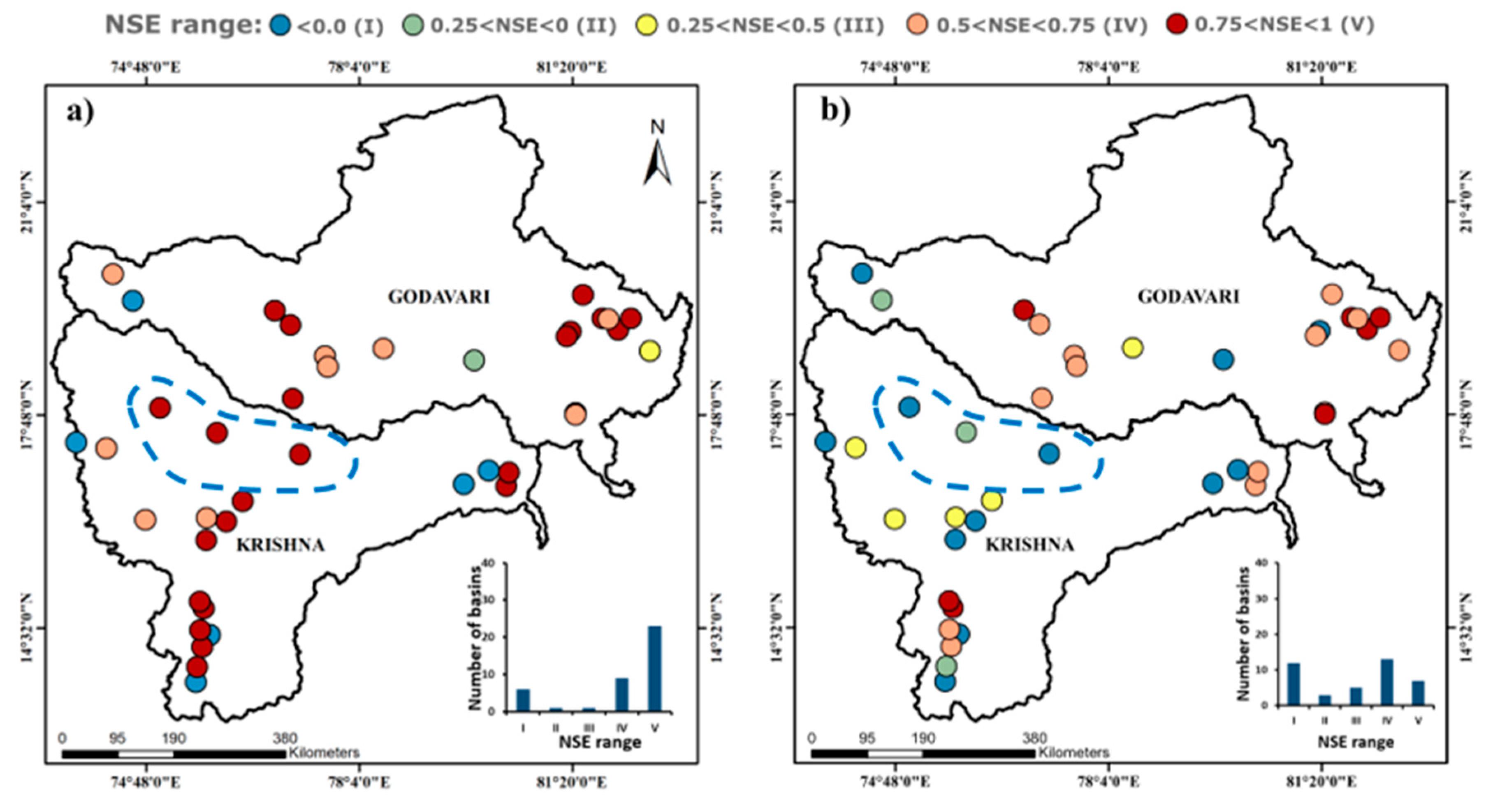
Figure 3 displays the FDCs predicted by the two models along with the observed FDCs for four sample basins (Ambabal, Honnali, Jagdalpur, and Kosagumda). It can be observed that for each of the four basins the FDC predicted by the DB model is closer to the observed FDC. In other words, as shown in Figure 4, discharge quantiles are usually better predicted by the DB model, which is highlighted by the fact that for all four basins is greater than . Figure 3 and Figure 4 give a general overview of the relative performances of the two models. is greater than in 33 out of the 40 study basins (see Figure 5 and Table S1). Furthermore, the 25th, 50th and 75th percentiles of and , considering the results from all 40 basins, are (0.61, 0.77, 0.89) and (−0.70, 0.48, 0.66), respectively. While these numbers indicate that the DB model is better than the IDW model at predicting FDCs in south India, an in-depth analysis is required to understand why the IDW model performed poorly. The IDW model has been applied to other datasets with better success rates (e.g., [9,52]).

Figure 3.
Comparison of observed and modelled FDCs for four sample basins: Ambabal (a), Honnali (b), Jagdalpur (c), and Kosagumda (d). It can be observed that for each of the four basins the DB model is better than the IDW model in predicting FDC.
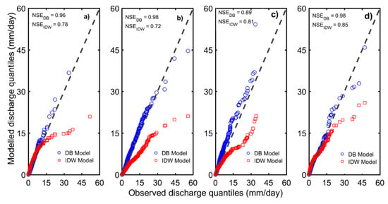
Figure 4.
Q‒Q plots for the four sample basins: Ambabal (a), Honnali (b), Jagdalpur (c), and Kosagumda (d). Observed discharge quantiles and modelled discharge quantiles are compared to evaluate the two models (the DB and the IDW) in terms of NSE. The four representative plots in the figure give an overall comparative assessment of the two models for the entire study region—the DB model is generally more reliable than the IDW model.
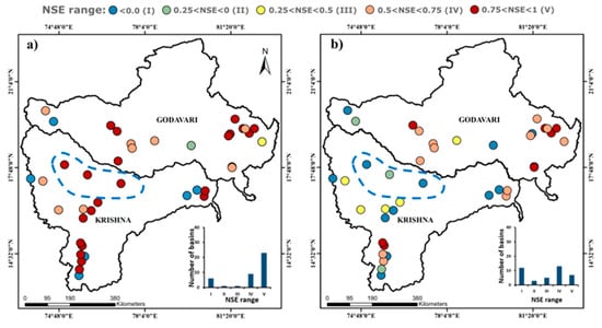
Figure 5.
Maps showing spatial distribution of (a) and (b), considering the results from all 40 study basins. The IDW model gives poor performance, particularly in places with low discharge gauging station density (compare the highlighted portions of the two maps), supporting the notion that regionalization models are unreliable in discharge data-scarce regions. The two insets are plots showing NSE range (see the legend on the top) vs. number of study basins, which provides a comparative assessment of the two models.
3.2. The IDW Model in Discharge Data-Scarce Situations
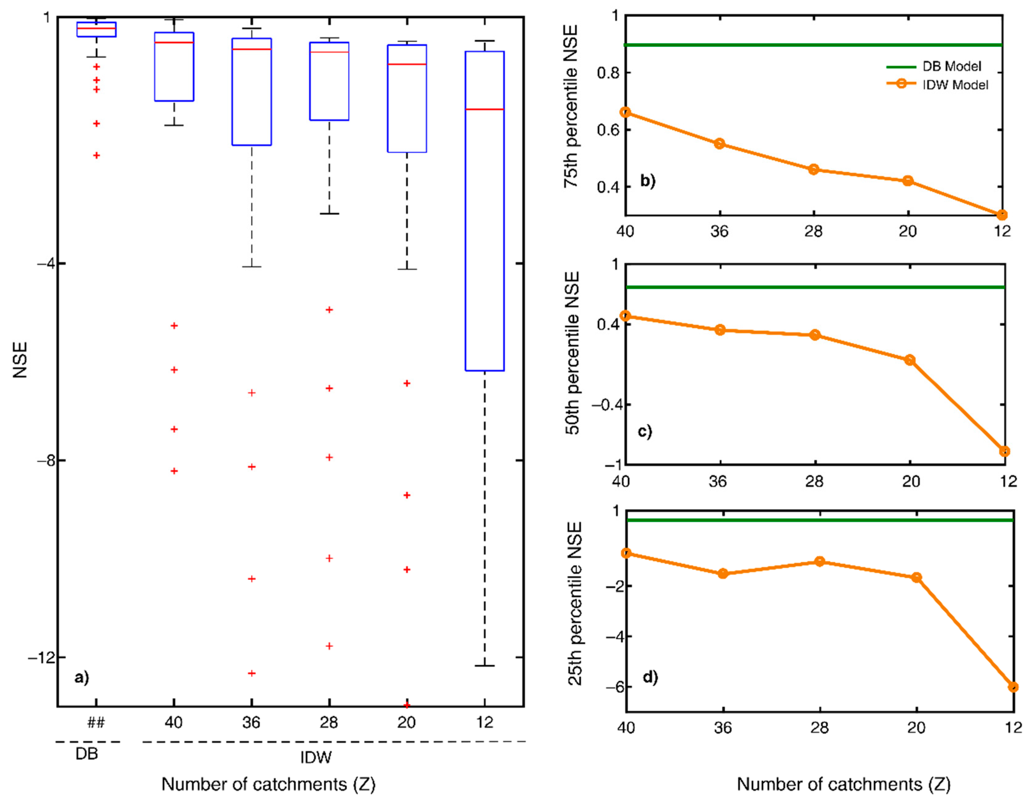
One reason behind the poor performance of the IDW model in the study region could be unavailability of adequate discharge data, as it is well known that regionalization method-based FDC models do not perform very well in regions with low discharge gauging station density [21]. The gauging station density in the study region (considering the 40 gauging stations) is approximately one gauging station per every 14,292 km2, in comparison to the global average of one station per 10,000 km2 [60]. It can be observed that in our study region is particularly low for the isolated gauging stations (see the highlighted portion in Figure 5b). Furthermore, the IDW model’s performance sharply declined as we removed gauging stations from input datasets, i.e., decreased with decreasing , the number of gauged basins considered for each test basin (Figure 6; for detailed methodology, see Section 2.3.1). Note that when . Figure 6b–d highlight how the 75th, 50th and 25th percentiles of decrease with decreasing . The results here thus reinforce the existing notion that regionalization method-based FDC models are unreliable in discharge data-scarce situations [22,23,24,50].
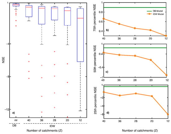
Figure 6.
Plots in this figure show the sensitivity of the IDW model’s performance () to discharge data scarcity. (a) Box plots of s for different values of , the number of gauged basins randomly selected for implementing the IDW model, considering results from all 40 study basins. For a comparison, the box plot also shows for the 40 study basins. The symbol ## in (a) corresponds to the fact that the DB model’s performance does not depend on . The remaining three plots show how the 75th percentile (b), 50th percentile (c) and 25th percentile (d) decline with (orange line). For comparison, each plot displays the corresponding values for the DB model (green lines). Overall, the figure suggests that regionalization models are unreliable in discharge data-scarce situations and that a calibration-free rainfall‒runoff model may be used in such situations.
We would also like to note that not all the basins have data for the same time period. One may thus argue this might be one of the reasons why the IDW model’s performance is not very satisfactory. However, we could not find a common time period for which all the study basins have discharge data. This, in fact, further strengthens our argument that the IDW model is sensitive to discharge data availability. On the other hand, the DB model’s performance is completely independent of discharge data availability as it does not require observed discharge data for predicting FDCs (see Figure 6). It can be applied in an ungauged basin using available meteorological information. For example, IMD provides gridded meteorological data for entire India for more than 100 years. Thus, a calibration-free rainfall‒runoff model may be preferred to predict FDCs in ungauged basins in regions such as India where discharge data are scarce but meteorological data are abundant. This argument is particularly relevant because streamflow gauging station density is currently in decline all over the globe, whereas it is becoming easier to obtain meteorological data even for the remotest locations due to advances in satellite remote sensing [26,27,28,29,30,31,61].
3.3. Influence of Observational Uncertainties on Model Performance
The unavailability of adequate observed discharge data may not be the only reason for the poor performance shown by the IDW model, as the quality of input data (discharge time series) also impacts performance of regionalization-based FDC models [21,25,62,63]. It is widely acknowledged that hydrological fluxes, measured using the most sophisticated instruments, can have significant error [41,43,64]. In this regard, it is noteworthy that the runoff ratio is greater than 1 for eight basins (not considered in the main analysis here; see Table S1) in the study region, which possibly indicates that data from these basins are highly erroneous, because the mean discharge does not exceed the mean rainfall in normal conditions. It is possible that some of the study basins satisfying our runoff ratio criteria (runoff ratio greater than 0.1 and less than 1) are also associated with significant observational errors. We would also like to mention here that the DB model’s performance is also expected to be sensitive to the quality of rainfall and PET data (the input data for the model), as gridded rainfall and PET data products are known to be associated with high observational errors [31,65,66,67]. In fact, it is also possible that some of the discarded basins (Table S1) did not satisfy our runoff ratio criteria because of significant errors in their rainfall time series. Another point that needs to be clarified here is that we have not considered anthropogenic activities in this study. Since activities such as construction of dams and barrages have the potential to alter streamflow patterns significantly, human influence might be one of the reasons the models did not perform optimally, particularly because most of our study basins are densely populated (e.g., [68]).
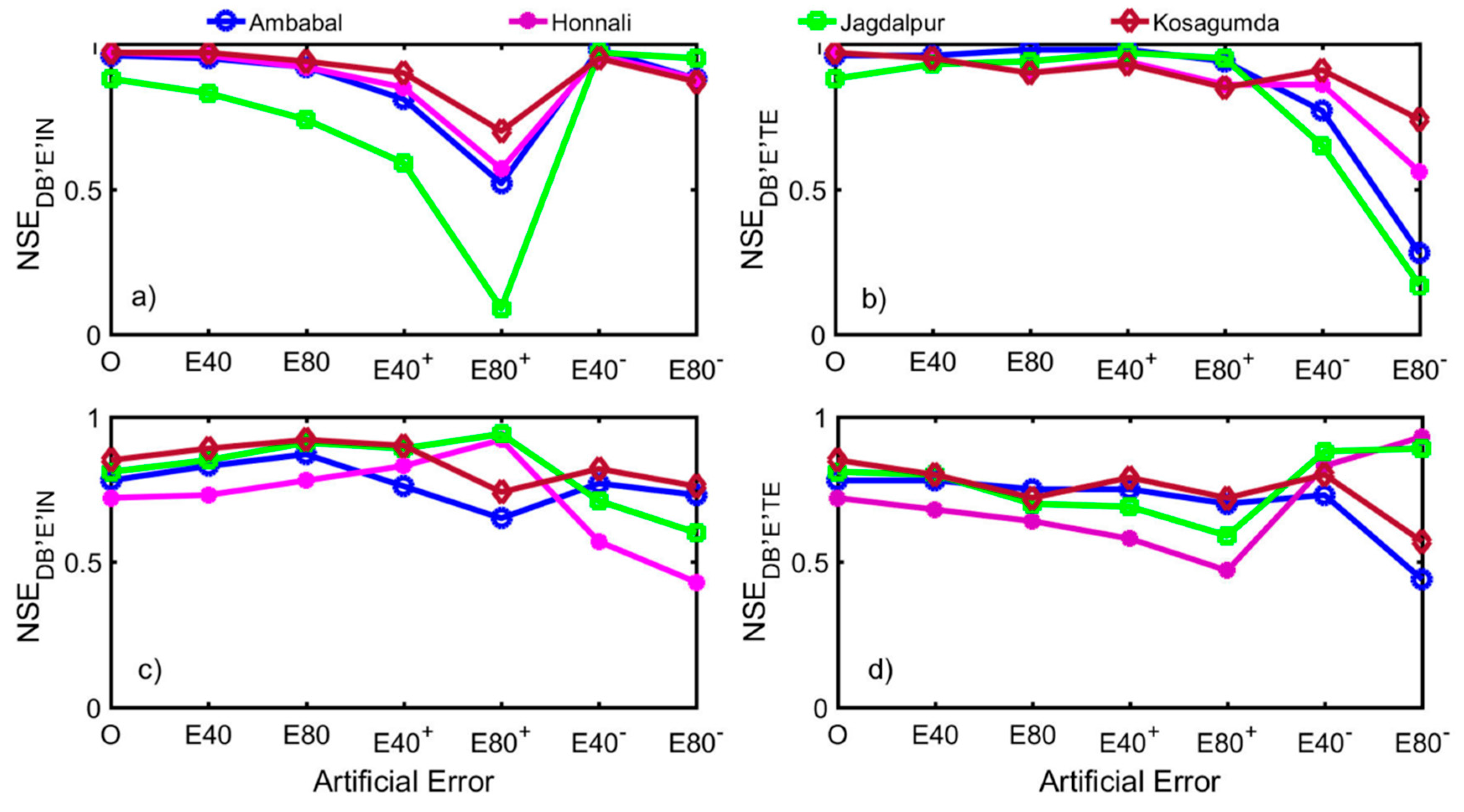
Although errors in input data influence the performance of both the models (Figure 7), it should be kept in mind that the two models use entirely different input datasets (the DB model requires only meteorological inputs, whereas the IDW model requires only discharge inputs). Thus, our observation—the overall performance of the DB model being better than that of the IDW model (Figure 3, Figure 4, Figure 5 and Figure 6)—might suggest that the discharge datasets are more erroneous than the meteorological datasets in our study region. This also means that the DB model is a better choice than the IDW model in regions where the meteorological datasets are less erroneous than the discharge datasets. Our analysis provides additional insight into how observational errors impact model performance. Firstly, how errors in input data will influence a model’s performance is quite unforeseeable (see how and respond to different error distributions in panels Figure 7a,c). We found that in certain cases model performance actually improves after the introduction of errors into input data (Figure 7). When a model’s baseline performance is low, it is more likely to be positively influenced by a skewed error distribution (see Figure 7). Perhaps when a model systematically underpredicts or overpredicts, errors in input data act as correction factors. Nevertheless, model performance cannot be improved by blindly introducing errors in input data as errors also influence model performance negatively. We would like to emphasize here that errors in test/validation data can also significantly influence model performance (Figure 7b,d), which also means that a low NSE does not necessarily imply poor model performance. The two models may have performed poorly in some of the study basins because of the poor quality of discharge data (test data) used for model evaluation. However, this is not a real concern for the DB model since it does not require discharge observations to predict FDCs in ungauged basins.
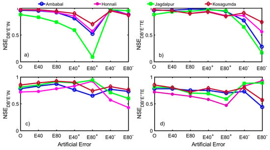
Figure 7.
Model performance is sensitive to observational errors for four sample catchments. (a,b) show DB model performance due to error () in input data () and test data (). Similarly, (c,d) show how and are sensitive to error in observed test data (discharge time series). For each experiment, six error distributions were considered (, , , , , and ). Each sample basin reacted to error distributions uniquely. Other basins of the study region displayed similar behaviour. Although errors in input data can negatively impact model performance, it should be noted that the two models used entirely different input datasets, and thus the choice of a particular model may be decided based on the quality of the available datasets. The figure also shows that a low NSE may not always imply poor model performance.
3.4. The Effect of Drainage Area on Model Performance
Drainage area can have a significant influence on model performance [69]. This phenomenon became apparent here when we divided the study basins into three groups according to their drainage area (each group having 10 study basins) and then viewed the s and s in box plots (Figure 8).

Figure 8.
Plots showing NSE box plots for the three groups of basins: small, medium and large. NSE box plots for the DB model (a) and the IDW model (b). The study basins are sorted into groups according to their drainage area, and each group has nearly the same number of basins. Note that basins with NSE less than −1 are not included in the plots as they are likely associated with significant observational errors. Although the patterns are not very clear, the two plots seem to offer some contrasting perspectives: the DB model’s performance improves with basin size, whereas the IDW model’s performance declines with drainage area.
Note that Figure 8 does not include basins for which both and are less than −1, as these basins are likely to be associated with observational errors significant enough to mask the NSE-drainage area relationships. The DB model’s performance was found to improve with catchment area (Figure 8a), which supports the earlier notion that continuous rainfall‒runoff models generally perform better in larger catchments [66]. This is likely because errors in input/meteorological data are smaller for larger basins due to the spatial aggregation effect [66,70,71,72]. This argument seems to be supported by the observation that the runoff ratio is greater than 1 for the two smallest basins (see Vandur and Ghargaon in Table S1). On the other hand, the IDW model’s performance declines with drainage area (Figure 8b). Again, this should not come as a surprise because, for a large basin, the discharge gauging station will be farther away from runoff source areas. Thus, as a cautionary note, the above observations suggest that the DB model’s advantage over the IDW model may diminish below a certain drainage area.
3.5. The Key to Better Hydrological Prediction: Process Understanding
There are many other regionalization-based models that one can use to predict FDC in an ungauged basin [14,15,52,59,73,74,75,76,77]. Some of them are arguably more powerful than the IDW model [9,13,51,52]. One may thus argue it is possible to find a regionalization-based FDC model that can predict FDCs more accurately in our study basins than the IDW model. However, our main argument is that regionalization-based FDC models may not be very useful when the discharge data are inadequate both quantitatively and qualitatively. In such a discharge data-scarce scenario, it will be more meaningful to use a calibration-free rainfall‒runoff model that predicts FDC using only meteorological information. This can, of course, be achieved if we have a calibration-free model that properly accounts for the hydrological processes responsible for transforming rainfall into streamflow. In this regard, it should be noted that many regionalization-based FDC models exploit meteorological information (along with discharge observations) for predicting FDCs in ungauged basins [76,78]. Nevertheless, we maintain that a calibration-free rainfall‒runoff model will still be more robust in cases of discharge data scarcity as it does not require discharge data in the first place. Furthermore, it is not very sensible to use regionalization models for predicting future FDCs when the climate is changing significantly, as the past discharge observations may not be useful anymore. A calibration-free model has an advantage in this scenario as it can directly utilize information provided by global circulation models to predict FDC. However, for accurately predicting the impact of climate change on a basin’s FDC, we may need to properly account for the vegetation dynamics caused due to climate change (e.g., [79,80]).
It is not a new practice to predict FDCs by explicitly accounting for hydrological processes (e.g., [1,23,81,82]). In fact, the DB model is not the only process-based calibration-free model capable of predicting FDCs in ungauged basins. Doulatyari et al. [1] developed a framework to predict FDCs without using observed discharge data by combining the following three models: the stochastic soil‒water balance model proposed by Botter et al. [81], the zero-parameter Budyko model [83] and the channel network morphology-based recession flow model proposed by Biswal and Marani [48]. Although a detailed assessment of the relative merits and demerits of these process-based FDC models is beyond the scope of this study, it should be emphasized here that this study employs a calibration-free dynamic rainfall‒runoff model for FDC prediction in ungauged basins for the first time. Our study stands apart even further if we consider the fact that attempts to exploit dynamic rainfall‒runoff models for FDC prediction in ungauged basins are “conspicuously absent” [22]. This is perhaps because there is no clear advantage of regionalizing the parameters of a typical dynamic rainfall‒runoff model, required for constructing FDCs in ungauged basins using meteorological data, over directly regionalizing flow quantiles. Lastly, the DB model may not be the ideal calibration-free dynamic rainfall‒runoff model. Future research may focus on developing more powerful calibration-free dynamic rainfall‒runoff models to predict FDCs in ungauged basins more accurately.
4. Summary and Conclusions
The construction of FDC is often a challenging task due to the unavailability of discharge data. The traditional answer to this problem is to transfer of information from gauged basins to ungauged basins following a regionalization method. However, it is widely known that regionalization method-based FDC models are not very reliable in regions with low gauging station density. Also, a regionalization-based FDC model is not expected to be effective when available discharge observations are poor in quality. In addition, regionalization-based FDC prediction is not very meaningful for a region witnessing significant climatic changes. Here we argue that the abovementioned challenges can be addressed, at least in part, by using a calibration-free dynamic rainfall‒runoff model that effectively utilizes available meteorological data to predict FDCs in ungauged basins. We test this hypothesis by comparing a recently proposed calibration-free dynamic rainfall‒runoff model (the DB model) with a well-known regionalization-based model (the IDW model) in south India, where discharge observations are not only inadequate quantitatively but also seem to be associated with significant errors.
The DB model outperformed the IDW model in 33 of the 40 study basins. The 25th, 50th and 75 percentile NSEs of the DB model, are 0.61, 0.77 and 0.89, respectively, which are significantly higher than those of the IDW model (−0.70, 0.48 and 0.66). Furthermore, the IDW model’s performance steeply declined as we randomly removed gauging stations from the input datasets to evaluate its performance in different discharge data scarcity scenarios. We also performed a detailed investigation on how the performance of the two models is affected by errors in data. Although in certain cases errors in data can actually influence model performance positively, data errors can have a strong negative impact on model performance (true for both models). Thus, the DB model may have a clear advantage over the IDW model only when the meteorological observations are less erroneous than the discharge observations. This scenario is now very common because it is becoming easier to obtain meteorological data even for remote regions due to advances in satellite remote sensing and numerical weather forecasting. We also found that the DB model’s performance improves with drainage area, while the IDW model’s performance declines with drainage area. Thus, caution should be exercised while selecting the DB model for predicting FDCs in smaller basins. Overall, our results suggest that the DB model is expected to be superior to the IDW model in regions where discharge data are inadequate not only quantitatively but also qualitatively. Some of the implications of our study are given as follows. We can predict FDCs for totally ungauged basins in discharge data-scarce regions using only meteorological data. The DB model provides a simple, yet effective, approach to explain hydrological processes occurring in drainage basins. Lastly, our study further strengthens the notion that the age-old Budyko framework is quite robust for modelling hydrological processes even at daily timescales (see [47]).
Supplementary Materials
The following are available at https://www.mdpi.com/2306-5338/6/2/32/s1. Table S1: Summary of the results from the study basins.
Author Contributions
Conceptualization, A.N. and B.B.; Data curation, A.N.; Formal analysis, A.N.; Investigation, A.N. and B.B.; Validation, A.N. and B.B.; Writing—original draft preparation, A.N.; Writing—review and editing, A.N. and B.B.; Supervision, B.B.
Acknowledgments
The authors would like to thank the Ministry of Human Resource Development (MHRD), India for funding Anita Nag’s doctoral research. Gridded meteorological rainfall and temperature datasets were obtained from the Indian Meteorological Department (IMD), Pune (detailed information on how to purchase the datasets is given at http://www.imd.gov.in/advertisements/20170320_advt_34.pdf). Discharge datasets were obtained from Krishna & Godavari Basin Organization (KGBO), Central Water Commission (CWC), Hyderabad (freely available on the India-WRIS website: (http://india-wris.nrsc.gov.in/wris.html). Digital elevation model data (DEM) for the basins were collected from the Consortium for Spatial Information (http://srtm.csi.cgiar.org/). The computer program to obtain spatial average rainfall and PET for the study basins from gridded IMD data was provided by Swagat Patnaik. The basin boundary shape files were prepared by Vimal Chandra Sharma.
Conflicts of Interest
The authors declare no conflict of interest.
References
- Doulatyari, B.; Betterle, A.; Basso, S.; Biswal, B. Predicting streamflow distributions and flow duration curves from landscape and climate. Adv. Water Resour. 2015, 83, 285–298. [Google Scholar] [CrossRef]
- Vogel, R.M.; Fennessey, N.M. Flow Duration Curves II: A Review of Applications in Water Resources Planning. J. Am. Water Resour. Assoc. 1996, 3, 1029–1039. [Google Scholar] [CrossRef]
- Mishra, A.K.; Coulibaly, P. Developments in hydrometric network design: A Review. Rev. Geophys. 2009, 47, 1–24. [Google Scholar] [CrossRef]
- Perumal, M.; Moramarco, T.; Sahoo, B.; Barbetta, S. A methodology for discharge estimation and rating curve development at ungauged river sites. Water Resour. Res. 2007, 43, 1–22. [Google Scholar] [CrossRef]
- Sivapalan, M.; Takeuchi, K.; Franks, S.W.; Gupta, V.K.; Karambiri, H.; Lakshmi, V.; Liang, X.; McDonnell, J.J.; Mendiondo, E.M.; O’connell, P.E.; et al. IAHS Decade on Predictions in Ungauged Basins (PUB), 2003–2012: Shaping an exciting future for the hydrological sciences. Hydrol. Sci. J. 2003, 48, 857–880. [Google Scholar] [CrossRef]
- Young, A.R. Stream flow simulation within UK ungauged catchments using a daily rainfall-runoff model. J. Hydrol. 2006, 320, 155–172. [Google Scholar] [CrossRef]
- Archfield, S.A.; Vogel, R.M. Map correlation method: Selection of a reference streamgage to estimate daily streamflow at ungaged catchments. Water Resour. Res. 2010, 46, 1–15. [Google Scholar] [CrossRef]
- Bloschl, G.; Sivapalan, M. Scale issues in hydrological modelling: A review. Hydrol. Process. 1995, 9, 251–290. [Google Scholar] [CrossRef]
- Castiglioni, S.; Castellarin, A.; Montanari, A. Prediction of low-flow indices in ungauged basins through physiographical space-based interpolation. J. Hydrol. 2009, 378, 272–280. [Google Scholar] [CrossRef]
- Hannaford, J.; Holmes, M.G.R.; Laizé, C.L.R.; Marsh, T.J.; Young, A.R. Evaluating hydrometric networks for prediction in ungauged basins: A new methodology and its application to England and Wales. Hydrol Res. 2013, 44, 401–418. [Google Scholar] [CrossRef][Green Version]
- He, Y.; Bárdossy, A.; Zehe, E. A review of regionalisation for continuous streamflow simulation. Hydrol. Earth Syst. Sci. 2011, 15, 3539–3553. [Google Scholar] [CrossRef]
- Razavi, T.; Coulibaly, P. Streamflow Prediction in Ungauged Basins: Review of Regionalization Methods. J. Hydrol. Eng. 2013, 18, 958–975. [Google Scholar]
- Samuel, J.; Coulibaly, P.; Metcalfe, R.A. Estimation of Continuous Streamflow in Ontario Ungauged Basins: Comparison of Regionalization Methods. J. Hydrol. Eng. 2011, 16, 447–459. [Google Scholar] [CrossRef]
- Shu, C.; Ouarda, T.B. Improved methods for daily streamflow estimates at ungauged sites. Water Resour. Res. 2012, 48, 1–15. [Google Scholar] [CrossRef]
- Waseem, M.; Ajmal, M.; Kim, T. Ensemble hydrological prediction of streamflow percentile at ungauged basins in Pakistan. J. Hydrol. 2015, 525, 130–137. [Google Scholar]
- Kokkonen, T.S.; Jakeman, A.J.; Young, P.C.; Koivusalo, H.J. Predicting daily flows in ungauged catchments: Model regionalization from catchment descriptors at the Coweeta Hydrologic Laboratory, North Carolina. Hydrol. Process. 2003, 17, 2219–2238. [Google Scholar] [CrossRef]
- Kumar, R.; Livneh, B.; Samaniego, L. Toward computationally efficient large-scale hydrologic predictions with a multiscale regionalization scheme. Water Resour. Res. 2013, 49, 5700–5714. [Google Scholar] [CrossRef]
- Seibert, J. Regionalisation of parameters for a conceptual rainfall-runoff model. Agric. For. Meteorol. 1999, 98, 279–293. [Google Scholar] [CrossRef]
- Yadav, M.; Wagener, T.; Gupta, H. Regionalization of constraints on expected watershed response behavior for improved predictions in ungauged basins. Adv. Water Resour. 2007, 30, 1756–1774. [Google Scholar] [CrossRef]
- Yokoo, Y.; Kazama, S.; Sawamoto, M.; Nishimura, H. Regionalization of lumped water balance model parameters based on multiple regression. J. Hydrol. 2001, 246, 209–222. [Google Scholar] [CrossRef]
- Hrachowitz, M.; Savenije, H.H.G.; Blöschl, G.; McDonnell, J.J.; Sivapalan, M.; Pomeroy, J.W.; Arheimer, B.; Blume, T.; Clark, M.P.; Ehret, U.; Fenicia, F. A decade of predictions in Ungauged Basins (PUB)—A review. Hydrol. Sci. J. 2013, 58, 1198–1255. [Google Scholar] [CrossRef]
- Castellarin, A.; Botter, G.; Hughes, D.A.; Liu, S.; Ouarda, T.B.M.J.; Parajka, J.; Post, D.A.; Sivapalan, M.; Spence, C.; Viglione, A.; et al. Prediction of Flow Duration Curves in Ungauged Basins. Runoff Prediction in Ungauged Basins: Synthesis Across Processes, Places and Scales; Cambridge University Press: Cambridge, UK, 2013; pp. 135–162. [Google Scholar]
- Müller, M.F.; Thompson, S.E. Comparing statistical and process-based flow duration curve models in ungauged basins and changing rain regimes. Hydrol. Earth Syst. Sci. 2016, 20, 669–683. [Google Scholar] [CrossRef]
- Patil, S.; Stieglitz, M. Controls on hydrologic similarity: Role of nearby gauged catchments for prediction at an ungauged catchment. Hydrol. Earth Syst. Sci. 2012, 16, 551–562. [Google Scholar] [CrossRef]
- Visessri, S.; McIntyre, N. Regionalisation of hydrological responses under land-use change and variable data quality. Hydrol. Sci. J. 2016, 61, 302–320. [Google Scholar] [CrossRef]
- Grimes, D.I.F.; Pardo-Iguzquiza, E.; Bonifacio, R. Optimal areal rainfall estimation using raingauges and satellite data. J. Hydrol. 1999, 222, 93–108. [Google Scholar] [CrossRef]
- Hou, A.Y.; Kakar, R.K.; Neeck, S.; Azarbarzin, A.A.; Kummerow, C.D.; Kojima, M.; Oki, R.; Nakamura, K.; Iguchi, T. The global precipitation measurement mission. Am. Meteorol. Soc. 2014, 95, 701–722. [Google Scholar] [CrossRef]
- Hughes, D.A. Comparison of satellite rainfall data with observations from gauging station networks. J. Hydrol. 2006, 327, 399–410. [Google Scholar] [CrossRef]
- Skofronick-Jackson, G.; Petersen, W.A.; Berg, W.; Kidd, C.; Stocker, E.F.; Kirschbaum, D.B.; Kakar, R.; Braun, S.A.; Huffman, G.J.; Iguchi, T.; Kirstetter, P.E. The global precipitation measurement (GPM) mission for science and society. Am. Meteorol. Soc. 2017, 98, 1679–1696. [Google Scholar] [CrossRef]
- Kummerow, C.; Barnes, W.; Kozu, T.; Shiue, J.; Simpson, J. The Tropical Rainfall Measuring Mission (TRMM) Sensor Package. J. Atmospheric Ocean. Technol. 1998, 15, 809–817. [Google Scholar] [CrossRef]
- Ward, E.; Buytaert, W.; Peaver, L.; Wheater, H. Evaluation of precipitation products over complex mountainous terrain: A water resources perspective. Adv. Water Resour. 2011, 34, 1222–1231. [Google Scholar] [CrossRef]
- Athira, P.; Sudheer, K.P.; Cibin, R.; Chaubey, I. Predictions in ungauged basins: An approach for regionalization of hydrological models considering the probability distribution of model parameters. Stoch. Environ. Res. Risk Assess. 2016, 30, 1131–1149. [Google Scholar] [CrossRef]
- Cutore, P.; Cristaudo, G.; Campisano, A.; Modica, C.; Cancelliere, A.; Rossi, G. Regional models for the estimation of streamflow series in ungauged basins. Water Resour. Manage. 2007, 21, 789–800. [Google Scholar] [CrossRef]
- McIntyre, N.; Lee, H.; Wheater, H.; Young, A.; Wagener, T. Ensemble predictions of runoff in ungauged catchments. Water Resour. Res. 2005, 41, 1–14. [Google Scholar] [CrossRef]
- Wagener, T.; Wheater, H.S. Parameter estimation and regionalization for continuous rainfall-runoff models including uncertainty. J. Hydrol. 2006, 320, 132–154. [Google Scholar] [CrossRef]
- Rajeevan, M.; Bhate, J.; Jaswal, A.K. Analysis of variability and trends of extreme rainfall events over India using 104 years of gridded daily rainfall data. Geophys. Res. Lett. 2008, 35, 1–6. [Google Scholar]
- Hargreaves, G.H.; Samani, Z.A. Reference Crop Evapotranspiration from Temperature. Appl. Eng. Agric. 1985, 1, 96–99. [Google Scholar] [CrossRef]
- Alexandersson, H. Korrektion av Nederbörd Enligt Enkel Klimatologisk Metodik: Correction of Precipitation According to Simple Climatological Principles; SMHI Meteorologi: Northkoping, Sweden, 2003. [Google Scholar]
- Baldassarre, G.D.; Montanari, A. Uncertainty in river discharge observations: A quantitative analysis. Hydrol. Earth Syst. Sci. 2009, 13, 913–921. [Google Scholar] [CrossRef]
- Dottori, F.; Martina, M.L.V.; Todini, E. A dynamic rating curve approach to indirect discharge measurement. Hydrol. Earth Syst. Sci. 2009, 13, 847–863. [Google Scholar] [CrossRef]
- Mcmillan, H.; Krueger, T.; Freer, J. Benchmarking observational uncertainties for hydrology: Rainfall, river discharge and water quality. Hydrol. Process. 2012, 26, 4078–4111. [Google Scholar] [CrossRef]
- Seibert, J.; Beven, K.J. Gauging the ungauged basin: How many discharge measurements are needed? Hydrol. Earth Syst. Sci. 2009, 13, 883–892. [Google Scholar] [CrossRef]
- Stephens, G.L.; Kummerow, C.D. The Remote Sensing of Clouds and Precipitation from Space: A Review. J. Atmos. Sci. 2007, 64, 3742–3765. [Google Scholar] [CrossRef]
- Viney, N.R.; Bates, B.C. It never rains on Sunday: The prevalence and implications of untagged multi-day-rainfall accumulations in the Australian high quality data set. Int. J. Climatol. 2004, 24, 1171–1192. [Google Scholar] [CrossRef]
- Mcmillan, H.; Freer, J.; Pappenberger, F.; Krueger, T.; Clark, M. Impacts of uncertain river flow data on rainfall-runoff model calibration and discharge predictions. Hydrol. Process. 2010, 24, 1270–1284. [Google Scholar] [CrossRef]
- Nruthya, K.; Srinivas, V.V. Evaluating Methods to Predict Streamflow at Ungauged Sites using Regional Flow Duration Curves: A Case Study. Aquat. Procedia. 2015, 4, 641–648. [Google Scholar] [CrossRef]
- Biswal, B. Dynamic hydrologic modeling using the zero-parameter Budyko model with instantaneous dryness index. Geophys. Res. Lett. 2016, 43, 9696–9703. [Google Scholar] [CrossRef]
- Biswal, B.; Marani, M. Universal’ recession curves and their geomorphological interpretation. Adv. Water Resour. 2014, 65, 34–42. [Google Scholar] [CrossRef]
- Rodriguez-Iturbe, I.; Rinaldo, A. Fractal River Basins: Chance and Self Organization; Cambridge University Press: Cambridge, UK, 1998; Volume 51, pp. 70–71. [Google Scholar]
- Oudin, L.; Andréassian, V.; Perrin, C.; Michel, C.; Le Moine, N. Spatial proximity, physical similarity, regression and ungaged catchments: A comparison of regionalization approaches based on 913 French catchments. Water Resour. Res. 2008, 44, 1–15. [Google Scholar] [CrossRef]
- Parajka, J.; Merz, R.; Blöschl, G. A comparison of regionalisation methods for catchment model parameters. Hydrol. Earth Syst. Sci. 2005, 9, 157–171. [Google Scholar] [CrossRef]
- Swain, J.B.; Patra, K.C. Streamflow Estimation in Ungauged Catchments Using Regional Flow Duration Curve: Comparative Study. J. Hydrol. Eng. 2017, 22, 04017010. [Google Scholar] [CrossRef]
- Shepard, D. A two-dimensional interpolation function for irregularly-spaced data. In Proceedings of the 23rd ACM National Conference, Association for Computing Machinery, New York, NY, USA, 27–29 August 1968. [Google Scholar]
- Nash, J.E.; Sutcliffe, J.V. River flow forecasting through conceptual models Part I-A discussion of principles. J. Hydrol. 1970, 10, 282–290. [Google Scholar] [CrossRef]
- Dulal, K.N.; Takeuchi, K.; Ishidaira, H. Evaluation of the influence of uncertainty in rainfall and discharge data on hydrological modeling. Annu. J. Hydraul. Eng. 2007, 51, 31–36. [Google Scholar] [CrossRef][Green Version]
- Mcmillan, H.; Jackson, B.; Clark, M.; Kavetski, D.; Woods, R. Input Uncertainty in Hydrological Models: An Evaluation of Error Models for Rainfall. J. Hydrol. 2011, 400, 83–94. [Google Scholar] [CrossRef]
- Oudin, L.; Perrin, C.; Mathevet, T.; Andreassian, V.; Michel, C. Impact of biased and randomly corrupted inputs on the efficiency and the parameters of watershed models. J. Hydrol. 2006, 320, 62–83. [Google Scholar] [CrossRef]
- Paturel, J.E.; Servat, E.; Vassiliadis, A. Sensitivity of conceptual rainfall-runoff algorithms to errors in input data- case of the GR2M model. J. Hydrol. 1995, 168, 111–125. [Google Scholar] [CrossRef]
- Zhang, Y.; Vaze, J.; Chiew, F.H.S.; Li, M. Comparing flow duration curve and rainfall–runoff modelling for predicting daily runoff in ungauged catchments. J. Hydrol. 2015, 525, 72–86. [Google Scholar] [CrossRef]
- Global Runoff Data Centre (GRDC) Status Report; World Meteorological Organization: Geneva, Switzerland, 2012; pp. 1–16.
- Woldemeskel, F.M.; Sivakumar, B.; Sharma, A. Merging gauge and satellite rainfall with specification of associated uncertainty across Australia. J. Hydrol. 2013, 499, 167–176. [Google Scholar] [CrossRef]
- Kjeldsen, T.R.; Jones, D.A. Predicting the index flood in ungauged UK catchments: On the link between data-transfer and spatial model error structure. J. Hydrol. 2010, 387, 1–9. [Google Scholar] [CrossRef]
- Merz, R.; Blöschl, G. Regionalisation of catchment model parameters. J. Hydrol. 2004, 287, 95–123. [Google Scholar] [CrossRef]
- Lee, J.; Shin, H.; Ahn, J.; Jeong, C. Accuracy Improvement of Discharge Measurement with Modification of Distance Made Good Heading. Adv. Meteorol. 2016, 2016. [Google Scholar] [CrossRef]
- Fawcett, R.; Trewin, B.; Barnes-Keoghan, I. Network-derived inhomogeneity in monthly rainfall analyses over western Tasmania. In Proceedings of the 17th National Conference of the Australian Meteorological and Oceanographic Society, Canberra, Australia, 27–29 January 2010. [Google Scholar]
- Raimonet, M.; Oudin, L.; Thieu, V.; Silvestre, M.; Vautard, R.; Rabouille, C.; Le Moigne, P. Evaluation of Gridded Meteorological Datasets for Hydrological Modeling. J. Hydrometeorol. 2017, 18, 3027–3041. [Google Scholar] [CrossRef]
- Tozer, C.R.; Kiem, A.S.; Verdon-Kidd, D.C. On the uncertainties associated with using gridded rainfall data as a proxy for observed. Hydrol. Earth Syst. Sci. 2012, 16, 1481–1499. [Google Scholar] [CrossRef]
- Shi, H.; Li, T.; Wang, K.; Zhang, A.; Wang, G.; Fu, X. Physically based simulation of the stream flow decrease caused by sediment-trapping dams in the middle Yellow River. Hydrol. Process. 2016, 30, 783–794. [Google Scholar] [CrossRef]
- Müller, M.F.; Thompson, S.E. TopREML: A topological restricted maximum likelihood approach to regionalize trended runoff signatures in stream networks. Hydrol. Earth Syst. Sci. 2015, 19, 2925–2942. [Google Scholar] [CrossRef]
- Merz, B.; Kreibich, H.; Schwarze, R.; Thieken, A. Review article Assessment of economic flood damage. Nat. Hazards Earth Syst. Sci. 2010, 10, 1697–1724. [Google Scholar] [CrossRef]
- Poncelet, C.; Merz, R.; Merz, B.; Parajka, J.; Oudin, L.; Andréassian, V.; Perrin, C. Process-based interpretation of conceptual hydrological model performance using a multinational catchment set. Water Resour. Res. 2017, 53, 7247–7268. [Google Scholar] [CrossRef]
- Esse, V.W.R.; Perrin, C.; Booji, M.J.; Augustijn, D.C.; Fenicia, F.; Kavetski, D.; Lobligeois, F. The influence of conceptual model structure on model performance: A comparative study for 237 French catchments. Hydrol. Earth Syst. Sci. 2013, 17, 4227–4239. [Google Scholar] [CrossRef]
- Boscarello, L.; Ravazzani, G.; Cislaghi, A.; Mancini, M. Regionalization of Flow-Duration Curves through Catchment Classification with Streamflow Signatures and Physiographic—Climate Indices. J. Hydrol. Eng. 2015, 21, 1–17. [Google Scholar] [CrossRef]
- Castellarin, A.; Vogel, R.M.; Brath, A. A stochastic index flow model of flow duration curves. Water Resour. Res. 2004, 40, 1–10. [Google Scholar] [CrossRef]
- Chokmani, K.; Ouarda, T.B.M.J. Physiographical space-based kriging for regional flood frequency estimation at ungauged sites. Water Resour. Res. 2004, 40, 1–13. [Google Scholar] [CrossRef]
- Mohamoud, Y.M. Prediction of daily flow duration curves and streamflow for ungauged catchments using regional flow duration curves. Hydrol. Sci. J. 2008, 53. [Google Scholar] [CrossRef]
- Skøien, J.O.; Merz, R.; Blöschl, G. Top-kriging—Geostatistics on stream networks. Hydrol. Earth Syst. Sci. 2006, 10, 277–287. [Google Scholar]
- Yaşar, M.; Baykan, N.O. Prediction of Flow Duration Curves for Ungauged Basins with Quasi-Newton Method. J. Water Resour. Prot. 2013, 5, 97–110. [Google Scholar] [CrossRef][Green Version]
- Wang, D.; Tang, Y. A one-parameter Budyko model for water balance captures emergent behavior in darwinian hydrologic models. Geophys. Res. Lett. 2014, 41, 4569–4577. [Google Scholar] [CrossRef]
- Zhang, S.; Yang, H.; Yang, D.; Jayawardena, A.W. Quantifying the effect of vegetation change on the regional water balance within the Budyko framework. Geophys. Res. Lett. 2016, 43, 1140–1148. [Google Scholar] [CrossRef]
- Botter, G.; Porporato, A.; Rodriguez-iturbe, I.; Rinaldo, A. Nonlinear storage-discharge relations and catchment streamflow regimes. Water Resour. Res. 2009, 45, 1–16. [Google Scholar] [CrossRef]
- Ceola, S.; Botter, G.; Bertuzzo, E.; Porporato, A.; Iturbe, I.R.; Rinaldo, A. Comparative study of ecohydrological streamflow probability distributions. Water Resour. Res. 2010, 46, 1–12. [Google Scholar] [CrossRef]
- Budyko, M.I. Climate and Life; Acdemic Press: New York, NY, USA, 1974. [Google Scholar]
© 2019 by the authors. Licensee MDPI, Basel, Switzerland. This article is an open access article distributed under the terms and conditions of the Creative Commons Attribution (CC BY) license (http://creativecommons.org/licenses/by/4.0/).

