A Conceptual Modeling Framework for Hydrologic Ecosystem Services

Abstract

Ecosystem services (ES) help people understand and deal with current environmental situations and problems, and ES-related research has been increasing recently. However, the quantitative evaluations of ES that can be easily understood by decision makers are still in development. Specifically, new methods are needed for hydrologic ES with the requirements of spatially and temporally explicit specification of parameters related to climate, geology, land cover, soil, and topography. This paper presents a conceptual modeling framework that aims to convert hydrologic information to hydrologic ES in fine temporal resolutions by developing a conceptual connection of three modules: data development, hydrologic and ES modeling, and results analysis. Then, the framework was applied to a study basin to demonstrate the importance of hydrologic ES in fine temporal resolutions. Results of water provision ES, flood control ES, and sediment regulation ES were produced at fine temporal resolutions in the framework, which indicates that more timely and relevant policy suggestions can be provided to decision makers. The framework and the methodology are applicable for watersheds of varied sizes and can serve as a template for future coupling of different environmental models.

1. Introduction

Human beings benefit enormously from the functions of ecosystems at various scales; such functions include the provision of food and resources, climate regulation, and recreational amenities [1]. The benefits that human beings obtain from ecosystems are referred to as ecosystem services (ES) [2]. Although studies have been conducted to identify and value ES over the decades, the development of assessment tools such as ES simulation models is still new [3]. Without quantitative evaluations of the actual benefits that can be obtained from ecosystems, the importance of these services does not draw adequate attention from decision makers [4].

Hydrologic ES, a subset of terrestrial ES related to water, are affected by complex interactions of many environmental factors and require a robust understanding and the skills for prediction and assessment [5]. Hydrologic models can simulate spatially and temporally explicit hydrologic processes, capture the heterogeneities in hydrologic and meteorological parameters, and enhance the understanding and prediction of hydrologic processes [6]. However, most hydrologic models are not designed to include functions that convert hydrologic results to the ES as easily understood by decision makers [5]. On the other hand, ES models are still under development, and hydrologic ES simulation is limited [5].

ES models and related quantitative research that have been built and conducted are limited in several ways. For example, the two ES models that have been mostly applied, Integrated Valuation of Ecosystem Services and Tradeoffs (InVEST) [7] and Artificial Intelligence for Ecosystem Services (ARIES) [8], are comprehensive ES models that cover many kinds and aspects of ES. However, neither of these two models uses temporally explicit methods to model the hydrologic ES, nor can they generate temporally explicit results. More importantly, temporal scales and resolution issues with ES modeling have not been studied in detail. The complex hierarchical organization of natural processes and heterogeneity across time and space make the scale of ecological research very important [9]. Furthermore, the beneficiaries of natural ES and their observation systems are in different spatial and temporal scales [10]. Most ecological functions are highly dynamic and nonlinear across space and time; however, such temporal nonlinearity has been ignored by previous studies without considering corresponding temporal scales to simulate the nonlinearity of ES [11].

Combining ES and hydrologic models can improve them both, which would effectively accelerate the ES modeling processes that need fine resolutions. Studies have been conducted to couple different types of hydrologic and ES models for hydrologic ES [12,13]. To achieve the goal of converting hydrologic information to ES with fine resolutions, we designed a conceptual modeling framework in this paper, including a data development function, a modeling function with a hydrologic model and an ES model, and a results analysis function. With this framework, we established procedures for hydrologic ES data preparation, simulation, and analysis supported by national geospatial data products. This framework could help decision makers and even the general public understand hydrologic ES. The framework was applied to a catchment with substantial urban land covers. In this paper, we evaluated three hydrologic ES variables at finer temporal resolutions than previous studies.

The first hydrologic ES variable is water provision ES. Limited studies have been conducted with a focus on water-related ES [14,15,16,17,18], with only a few of them on a seasonal or monthly basis [19,20]. Compared to Notter et al. [19], who used monthly hydrologic results to calculate the ES indices, this study not only uses daily hydrologic data but also produces monthly and seasonal ES indices which can provide more detailed information for decision makers. Similar to Schmalz et al. [20], the seasonal ES has been calculated to capture the high and low water provisions in different seasons. Furthermore, this study also compares annual and monthly changes to highlight the necessity of fine temporal results.

The second hydrologic ES variable is flood regulation ES. Because floods have short time frames, annual results may not be adequate for management activities. With the ability of this framework to simulate monthly and seasonal ES output, these extreme events could be captured and related remedies could be designed. Unlike previous ES studies [16,21], the flooding regulation ES simulated in this study can not only predict the flooding risk per year but also pinpoint the months and seasons when regulation for ES should be applied.

The third hydrological ES variable is sediment regulation ES. When it comes to sediment retention, even if sediment yields were low in a year, they could be quite high in some months; thus, attention should be given to such months. Previous ES studies focused on sediment regulation with annual outputs [14,15,21]. In general, they tested different land-use scenarios on the study areas to calculate different sediment yields for comparison and tradeoff, neither of which captures the seasonal changes in sediment associated with extreme hydrologic events nor provides guidance as in this study and that of Schmalz et al. [20].

In short, this study focused on finding the changes in hydrologic ES at fine temporal resolutions compared to previous hydrologic ES studies. As mentioned earlier, ES models (e.g., InVEST) were limited to the annual scale with their design, and most of the studies focused on the tradeoff of different land use scenarios or mapping the spatial distribution of ES [4,14,15,18]. Other hydrologic models (e.g., Soil & Water Assessment Tool (SWAT)) capable of simulating hydrologic variables at fine temporal resolutions were also utilized in previous studies [19,20,21], but only Schmalz et al. [20] conducted their study at the seasonal scale and the smallest hydrologic unit in SWAT. Thus, further studies at fine temporal resolutions in hydrologic ES are still needed.

The novelty of our work lies in developing the conceptual framework and demonstrating the importance of evaluating hydrological ES at fine temporal resolutions compared to previous studies [20]. The results of the framework showed that hydrologic ES were temporally sensitive, and with this conceptual modeling framework, these fine temporal changes could be captured and relevant management plans and policies could be made accordingly.

The upcoming sections of this article provide details of our framework. In Section 2, we introduce hydrological and ES models used for the framework and explain each function in the framework. We also describe data sources and the study site in Section 2. Results and discussion for each ES variable are provided in Section 3, followed by conclusions in Section 4.

2. Materials and Methods

2.1. Hydrologic Model

The Hydrologic Simulation Program-Fortran (HSPF) [22] was employed in this study to simulate streamflow and sediment yields. HSPF is a comprehensive, physically based, semi-distributed hydrological model [23]. It has been applied to study hydrological variables such as streamflow, sediment yield, and nonpoint source pollution in many projects conducted around the world, e.g., [24,25,26,27,28,29].

In HSPF, the study area is first divided into subbasins according to topography as each subbasin is the smallest catchment that contains a stream channel with no branch [23]. Each subbasin is configured to have three basic components, namely pervious land segments (PERLND), impervious land segments (IMPLND), and stream channel/reservoir (RCHRES) [23]. Land surface processes are simulated for PERLND and IMPLND first. Simulation results from PERLND and IMPLND are then passed to RCHRES for channel/reservoir or hydraulic processes simulation. With land use/cover, imperviousness, climate, reaches, and subbasin data, the hydrologic modeling function will be set up. The PERLND, IMPLND, and RCHRES are assigned based on subbasin delineation, land use/cover types, weather stations, and the ratio of perviousness and imperviousness for each land use/cover type. The geometric and hydraulic properties of an RCHRES are represented in HSPF by an FTABLE, which describes the relationships between stage, surface area, volume, and discharge for the reach segment.

The hydrologic processes of the model are based on the water-balance equation (Equation (1)).

$$SM{C}_t=SM{C}_{t-1}+{{\displaystyle \sum }}_{t=1}^T\left(P_t-R_t-E{T}_t-G_t\right)$$

(1)

where SMC is the soil moisture content, t is time in days, T is the total days, P is the daily amounts of precipitation, R is the runoff, ET is the actual evapotranspiration, and G is the deep groundwater (percolation). All of the units are in mm.

The data products we used for HSPF are listed in

Table 1. Summary of data sets used for hydrological modeling.

Data sets	Spatial Resolution	Source
Digital elevation data	30 m	US Geological Survey (USGS) [30]
Land cover map	30 m	National Land Cover Database (NLCD) [31]
Climate data	8 km	University of Wisconsin-Madison [32]
Streamflow and sediments yield data	N/A	USGS [33]

.

The model parameters were calibrated against the measured streamflow data for the period 1986–1995 and were subsequently validated for the period 1996–2005 in the previous study [21]. The calibration period was selected considering the timing of the National Land Cover Database (NLCD) data and the availability of streamflow data. The comparison with the measured streamflow was conducted in terms of relative error (RE) and the Nash–Sutcliffe Efficiency (NSE). Sediment data have very limited availability; thus, available daily numbers were averaged to monthly ones and compared with simulated results.

2.2. ES Model and Methods

To evaluate ES, quantitative methods created by Logsdon and Chaubey [21] were used with modifications to configure the fine temporal resolution requirement. In this paper, the time step was a day, and the results were analyzed both monthly and seasonally to illustrate the change of water demand throughout the year.

2.2.1. Water Provision ES

The water provision ES was calculated as the index of water provisioning (WPI) (Equation (2)).

$$WP{I}_t= \frac{M{F}_t/M{F}_{EF}}{M{F}_t/M{F}_{EF}+qn{e}_t/n_t}$$

(2)

where WPI is water provision index at time t, MF is the mean flow (m³/s), MF_EF is the long-term environmental flow requirement (m³/s), qne is the number of times the flow is less than environmental flow requirements in the time step, and n is the total number of units in the time step.

The WPI equation adopted in this study does not include water quality index (due to the data scarcity) unlike the original equation developed by Logsdon and Chaubey [21]. The WPI ranges from 0 to 1, where 0 indicates that the provision of water quantity is not met at all, and 1 indicates that the provision of water quantity is met for the entire period of time. Based on Tennant [34], 30% of the average flow for each month was used as MF_EF to sustain good aquatic ecosystem functioning. The qne value was calculated on a daily basis.

We then grouped individual monthly WPI numbers into three categories with respect to the mean and standard deviation to examine the distribution of monthly WPI numbers. Category A is for those above the mean by one standard deviation or more, category B is for those within one standard deviation from the mean, and category C is for those below the mean by one standard deviation or more.

2.2.2. Flood Regulation ES

The flood regulation ES was calculated as the flood regulation index (FRI). FRI incorporates three flood characteristics—quantity, duration, and extent of the flooding [35]—and is calculated according to Equation (3).

$$FRI=\frac{1}{\exp [w_1·\left(DF/D{F}_{LT}\right)+w_2·\left(QF/Q{F}_{LT}\right)+w_3·\left(FE/F{E}_{LT}\right)]}$$

(3)

where DF is the duration of flood events (days), QF is the average magnitude of flooding events (m³/s), FE is the number of flood events per month or year, w₁, w₂, and w₃ are user-designed weights for each component of flooding (the sum of the weights is 1), and the LT subscript represents long-term (historical) data.

The FRI ranges from 0 to 1, with 0 representing the maximum regulation needed and 1 representing no regulation needed. As discussed in the introduction section, flood-regulation ES is time-sensitive. With this adopted method, the FRI will be calculated for each month with daily data to highlight seasonal changes in flood events and their effects. Long-term, observed, streamflow data from the study area were used to determine the flood flow (calculated as the 10th percentile of the flow), which then was used to calculate the long-term values for the average duration of flood events, average magnitude of flood events, and average number of flood events per year.

The individual monthly FRI numbers were then divided into two categories: A (FRI = 1 as no flood) and B (FRI < 1 as flood events) for further analysis.

2.2.3. Sediment Retention ES

The sediment retention ES was calculated as the sediment regulation index (SRI), which is defined in Equation (4):

$$SRI=\exp \left(1-\left(S/S_{max}\right)\right)$$

(4)

where S is the monthly/annual erosion rate (T/ha) and S_max is the monthly/annual maximum allowable (or natural) rate of sediment (T/ha).

The range of SRI is 0 to infinity. When the monthly sediment equals to or is less than the allowable sediment, the SRI is equal to or larger than 1, meaning no regulation is needed. If the sediment is greater than the maximum allowable sediment, the ERI is less than 1, indicating that sediment regulation is needed. The maximum allowable sediment load used was the area-weighted US Department of Agriculture ‘T’ factor for tolerable soil loss [36]. It was determined to be 1.34 T/ha/year and then converted to monthly data, weighted by flow data.

The counts of SRI by month were then grouped into three categories: A is for those above the mean by one standard deviation or more, B is for those within one standard deviation from the mean, and C is for those below the mean by one standard deviation or more.

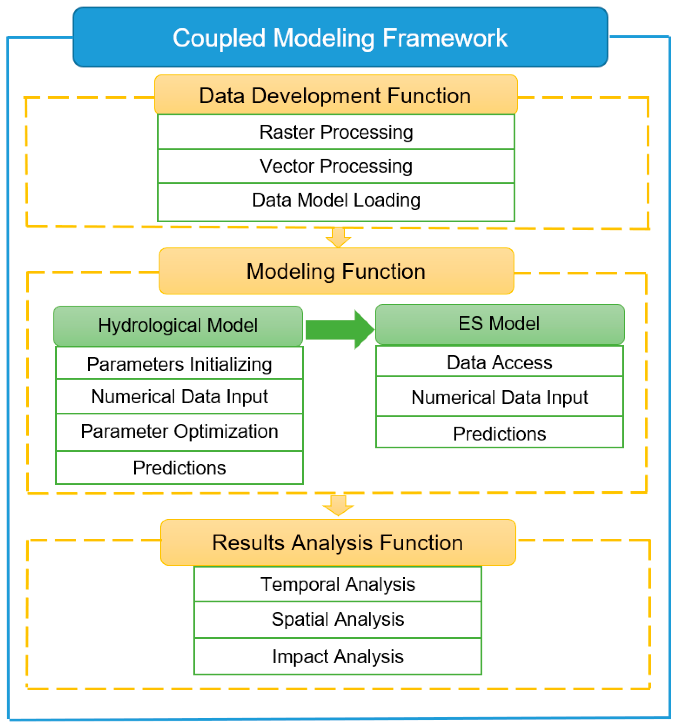
2.3. The Conceptual Framework and Workflow

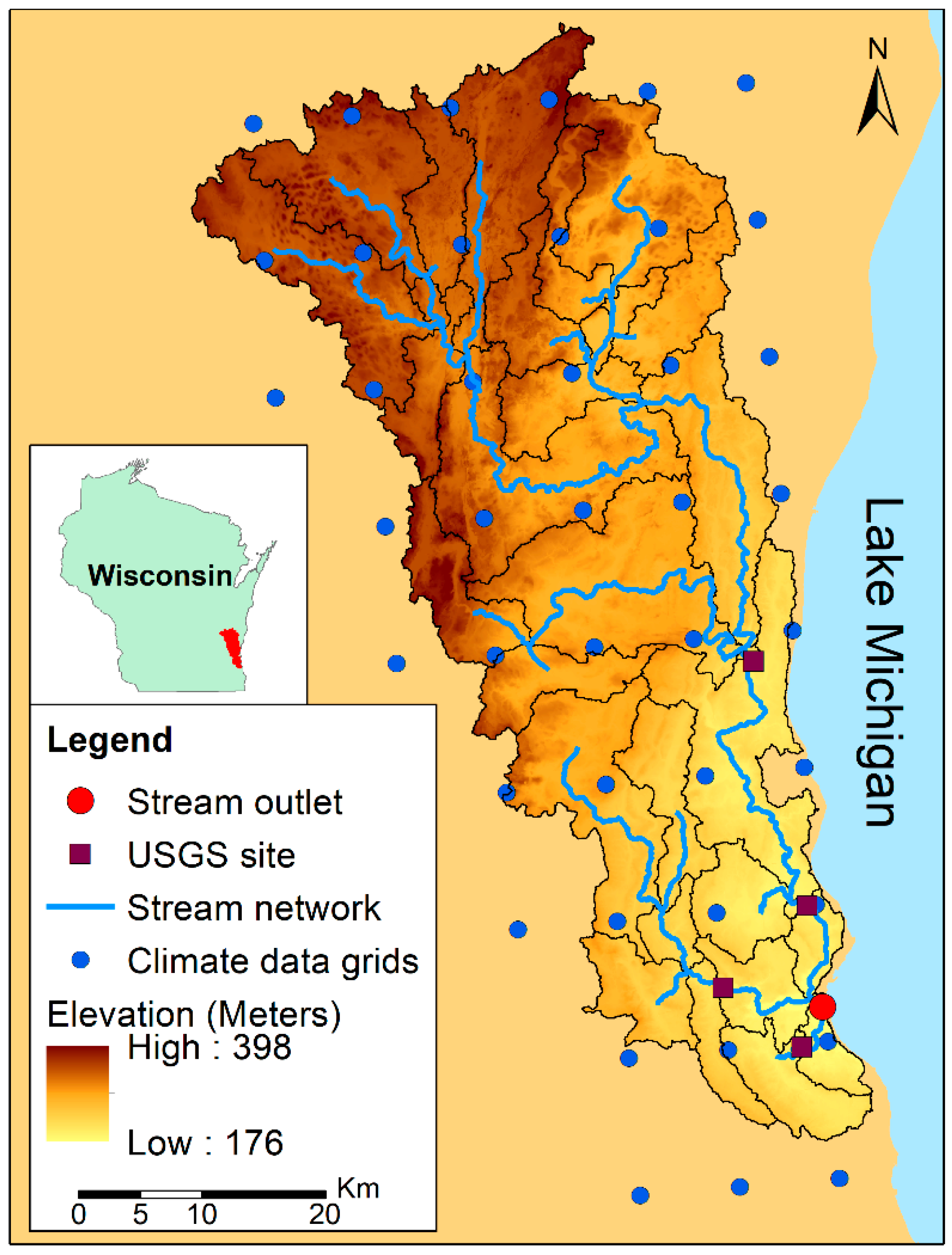
The complete conceptual workflow of the framework is portrayed in Figure 1. The framework consists of three main functions, namely data development, modeling, and results analysis, each of which is further described below.

In the data development function, digital elevation model (DEM) data were used to create a watershed boundary and stream network. Then, the watershed boundary, weather station map, imperviousness map, land use/cover map, and stream network were used to assign properties for each subbasin and stream segment. At the end, all the data were inputted to the data model loader for initializing the hydrologic model.

The modeling function has two components: hydrological and ES models. In this study, hydrological model (HSPF) outputs were fed into the three hydrological ES models described previously. In the hydrologic model, with the data from the data development function, all the parameters were initialized with default values and some numerical data were manually input. Then, the model was calibrated against the observed data by optimizing sensitive parameters, and the simulations were conducted with the best combination of parameters. In the ES model, the three ES were simulated with the hydrologic outputs and other manually inputted data.

In the results analysis function, the hydrologic ES results were produced as grids and then aggregated to subbasin and basin scales for different research purposes. With regard to temporal scales, the results were calculated in daily steps and then aggregated to monthly and annual scales for different purposes. This paper presents an example of results at different temporal scales.

Furthermore, an impact analysis can be conducted by adopting various scenarios such as climate change and land use/cover change.

2.4. Study Area

We tested the framework for the Milwaukee River basin (Figure 2), which includes 13 cities, 32 towns, and 24 villages. The total population of the basin is about 1.3 million, and the basin area is about 2267 km². The southeast part, where the city of Milwaukee is located, is the most densely populated and urbanized area in the state, whereas the land cover in the northern portion consists primarily of agricultural land. Across the basin, predominant land cover types include forest (11%), wetland (12%), planted/cultivated (43%), and urban (32%). The basin has topography comprised of rolling moraine over bedrock, and it slopes downward from northwest to southeast, exiting to Lake Michigan [37].

3. Results and Discussion

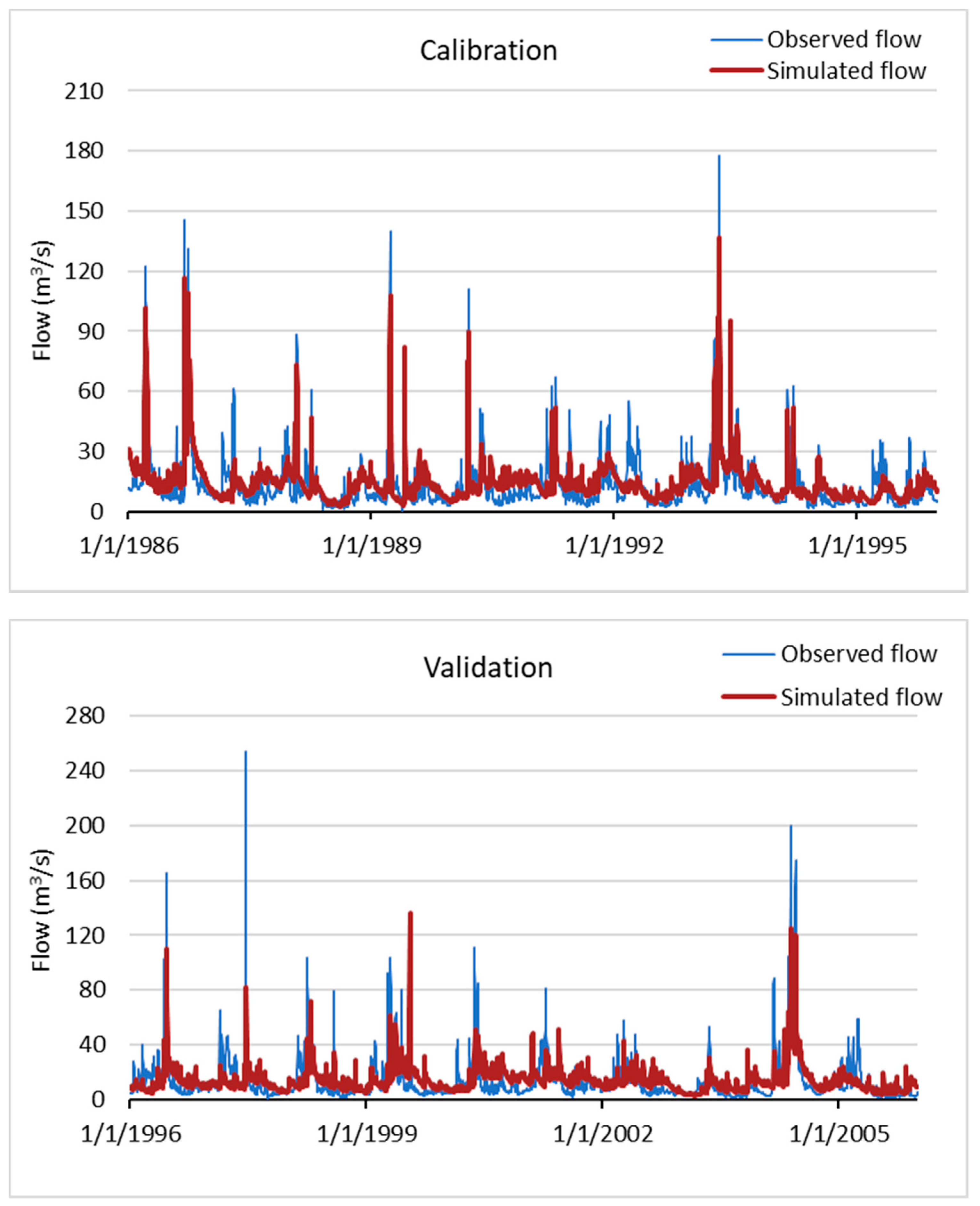
3.1. Hydrological Modeling

For the calibration period, the RE was 2.13% and the NSE was 0.71 at the USGS streamflow measurement site (site number 04087000, the second one from north in Figure 2). They were 4.87% and 0.54 for the validation period, respectively. The time series of observed and simulated flow are shown in Figure 3. Overall, the results of streamflow calibration and validation show good performance of the HSPF model.

The simulated and measured total suspended solids were then compared on monthly and annual bases (see Figure 4) without calibration since daily measurements were not available. The RE numbers at annual and monthly scales are 3.26% and 9.57%, respectively. The comparison indicates overestimation at both monthly and annual scales, whereas the monthly simulations show larger overestimation.

3.2. Ecosystem Services Modeling

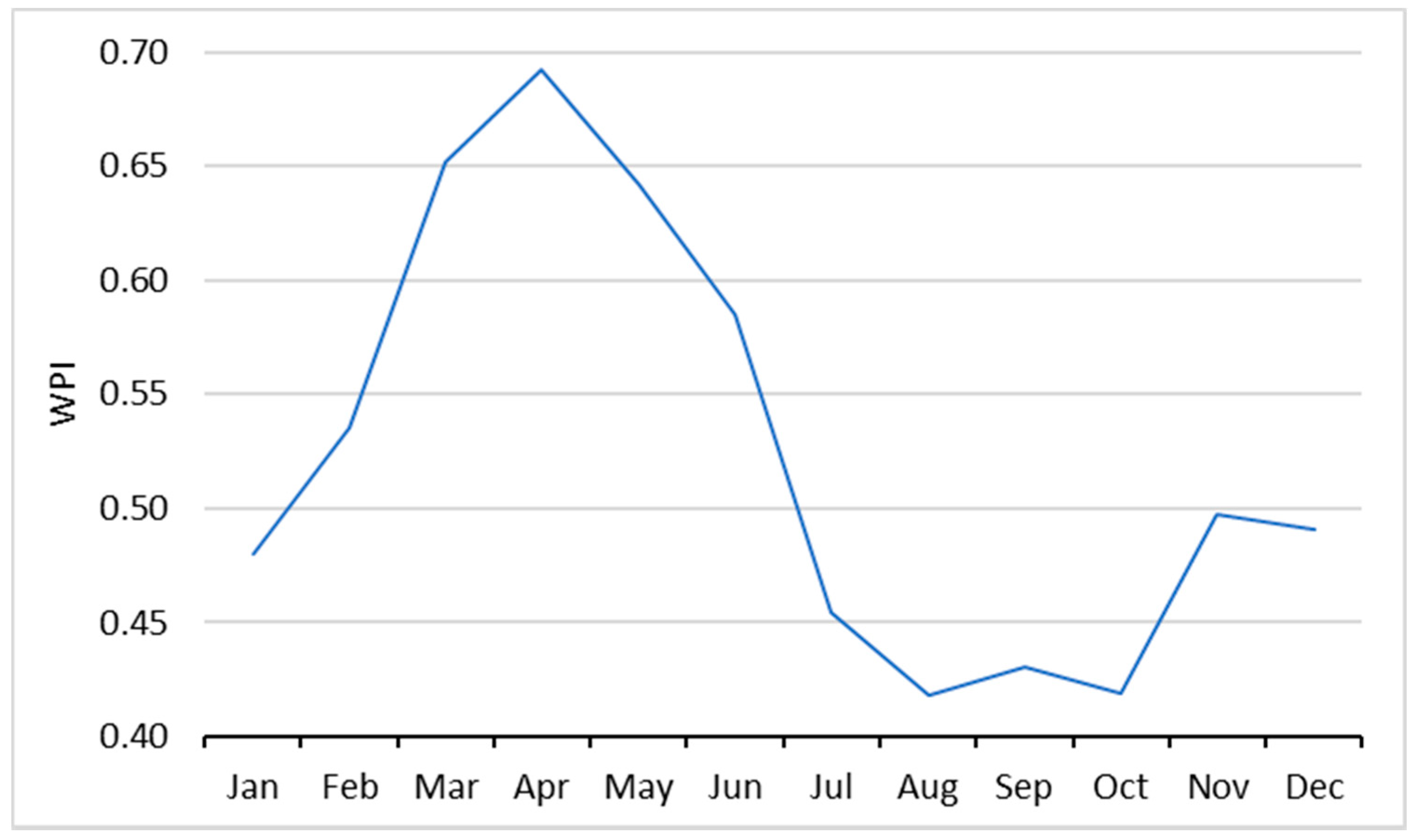
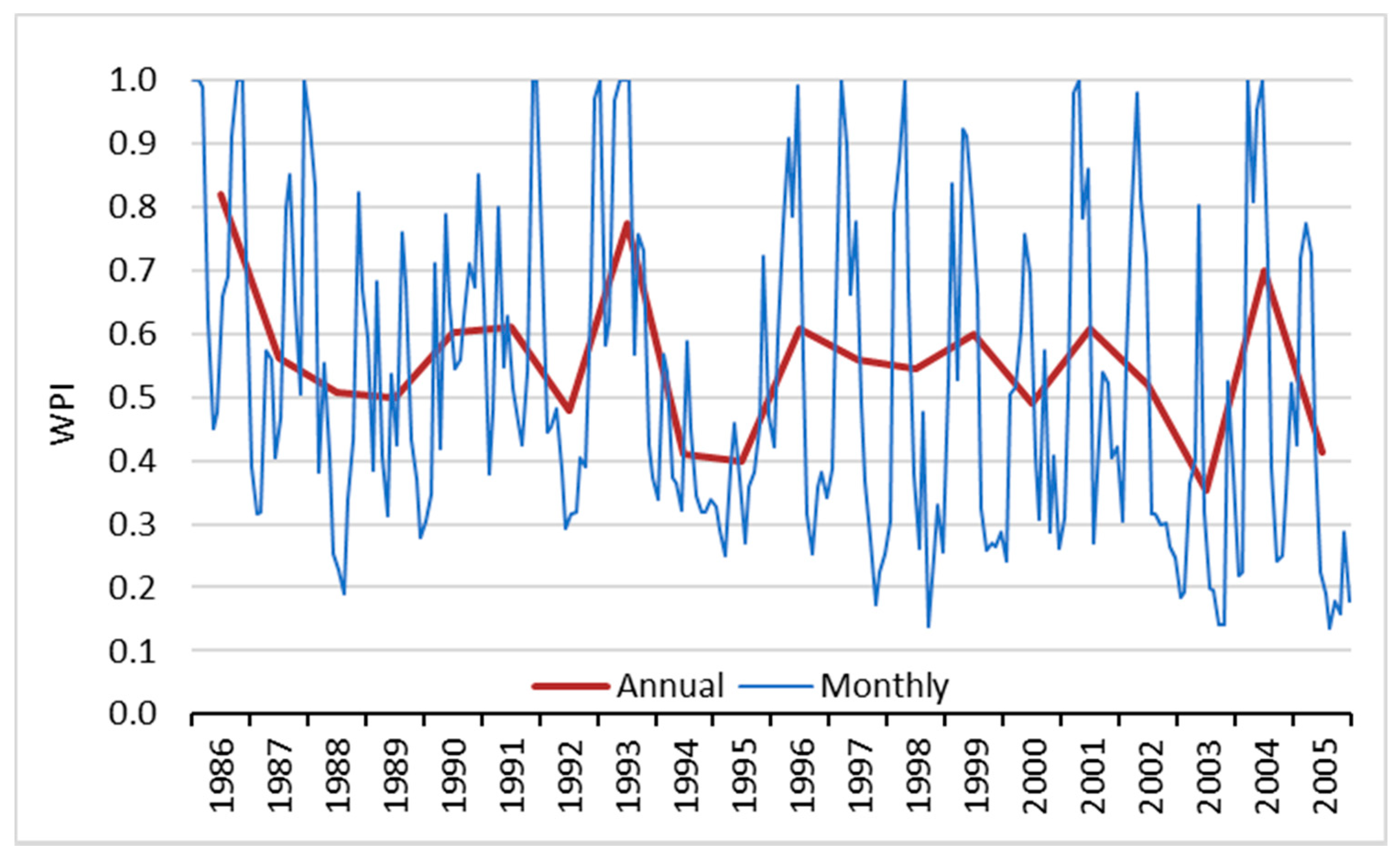
3.2.1. Water Provision Index (WPI)

The WPI (Equation (2)) was calculated both as annual and monthly time series for the entire basin (Figure 5). The annual WPI ranges between 0.35 and 0.85 and reveals a slightly decreasing trend during the study period. The diminished water provision could be caused by some natural processes such as reduced precipitation, increased evaporation, and/or water table depression, as well as some human effects such as overconsumption of water for domestic or industrial use. The monthly WPI fluctuates wildly, between less than 0.2 and 1.0, and monthly WPI numbers below 0.2 occur more frequently in the second half.

We would like to further highlight some notable differences between annual and monthly results in Figure 5. For example, in the years 1986 and 2004, the annual WPI was very high, but the monthly WPI was very low in the late summer of those years. The monthly WPI in those years was as low as those when the annual WPI was quite low, such as in the periods 1987–1988 and 2002–2003. In the years 1988, 1998, and 2003, the annual WPI was low but the monthly WPI in the late spring or early summer of those years was very high even compared to some years (such as 1986 and 2004) with a high annual WPI. These findings indicate that annual WPI alone cannot provide enough or adequate information about when the shortages occur.

The monthly WPI time series was converted to the mean monthly WPI (Figure 6) to examine the seasonal variability in the study basin. Figure 6 reveals high water provisions in spring and very low water provisions in summer. Given the results at different temporal resolutions of the water provisions, the management plan for this basin could focus on low-flow seasons to keep the level of water provision stable.

The category counts described in Section 2.2.1 for each month are provided in

Table 2. Counts of monthly water provision index numbers above the mean by one standard deviation or more (A), within one standard deviation from the mean (B), and below the mean by one standard deviation or more (C).

	Category	A	B	C
Month
Jan		3	14	3
Feb		4	14	2
Mar		8	11	1
Apr		9	11	0
May		8	12	0
Jun		6	12	2
Jul		1	13	6
Aug		1	16	3
Sep		2	11	7
Oct		1	13	6
Nov		3	14	3
Dec		4	10	6

. For category A, spring (March to May) has the most counts, and for category C, spring has the least counts, which indicates high water provision in spring. Category A has the least counts and Category C has the most counts in summer and early autumn (July to Oct), which indicates low provision in this season. This further demonstrates that monthly results can provide information for water provision management considering seasonal variations.

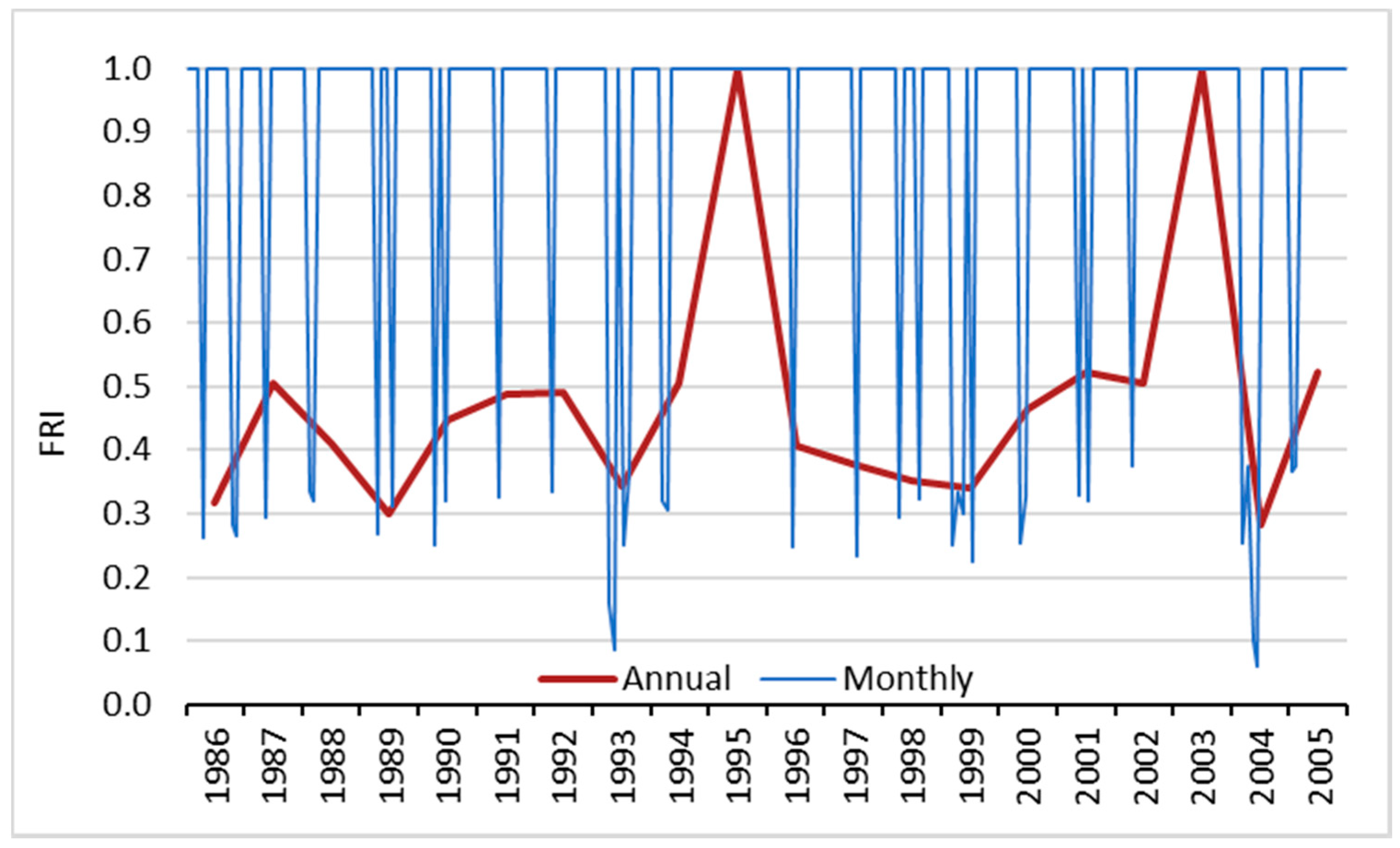
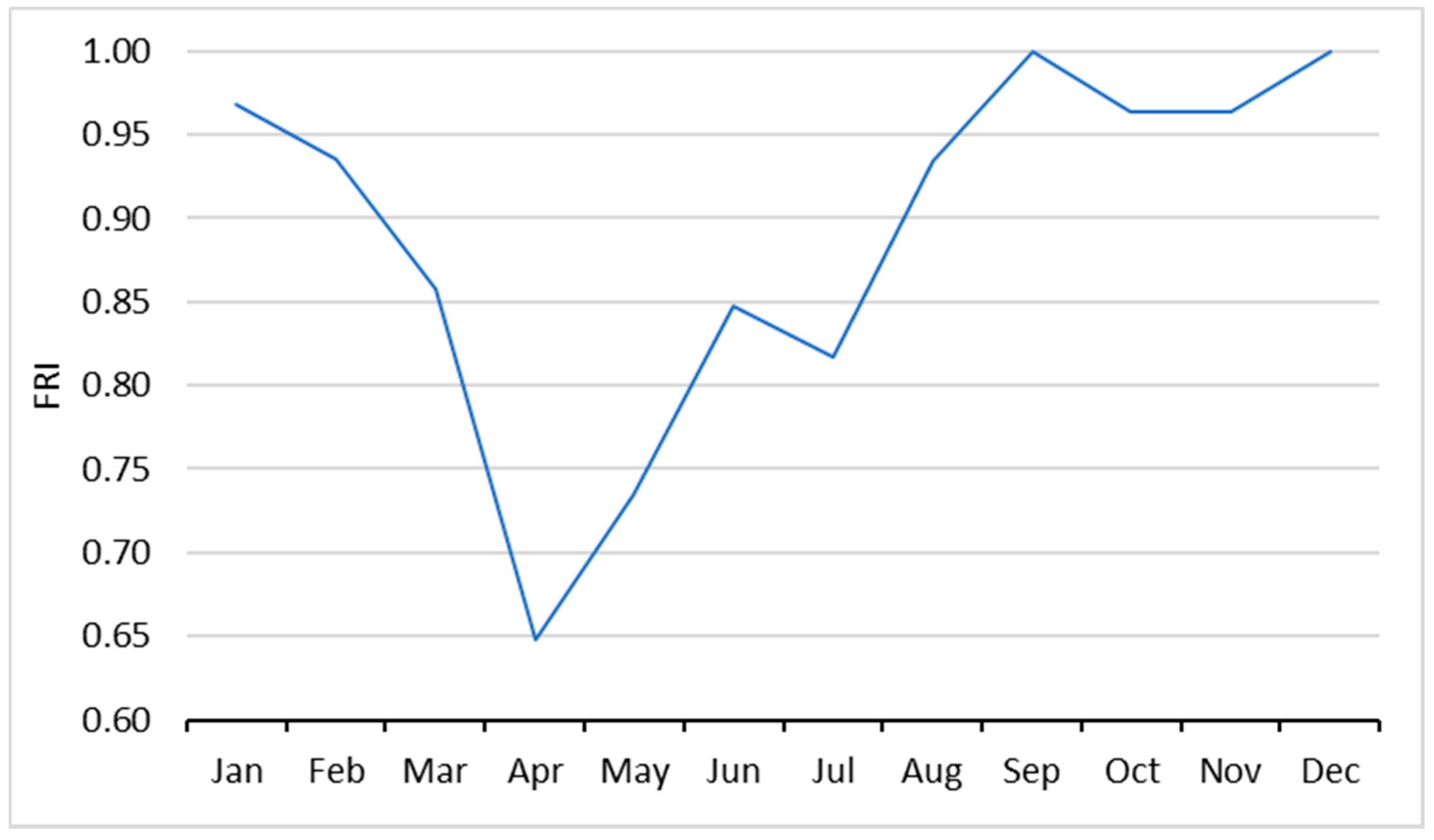
3.2.2. Flood Regulation Index (FRI)

The FRI (Equation (3)) was calculated as both annual and monthly time series (Figure 7), and mean monthly as well (Figure 8). As mentioned before, 0 represents the maximum regulation needed and 1 represents no needed regulation.

The annual FRI (Figure 7) mostly hovers around 0.4–0.5, which indicates that management is needed to some extent to regulate the flood effects most of the time. However, the monthly FRI numbers are 1 most of the time and very low occasionally, which means no flood regulation is needed for most of the time. The monthly FRI shows that flood regulations were not required except for certain months. Equation (3) indicates that the magnitude and duration of flood events highly impact FRI. These findings reveal that further flood regulation will only be needed for certain months or seasons. Annual results were not adequate for the flood regulation management plans.

Figure 8 reveals that spring is the time when the study basin is most vulnerable to flooding, while winter is relatively safe from flooding. The category counts described in Section 2.2.2 are provided in

Table 3. Counts of flood regulation index numbers equal to 1 (A) and less than 1 (B).

	Category	A	B
Month
Jan		19	1
Feb		18	2
Mar		16	4
Apr		10	10
May		13	7
Jun		16	4
Jul		15	5
Aug		18	2
Sep		20	0
Oct		19	1
Nov		19	1
Dec		20	0

for each month. Together with Figure 8, these results indicate that the study area is subject to more flood events from March to July compared to other seasons. Thus, decision makers should establish some seasonal and temporary management (e.g., moveable dams) to prevent or reduce flood duration and magnitude, and such controls should be implemented for the spring and early summer in the future.

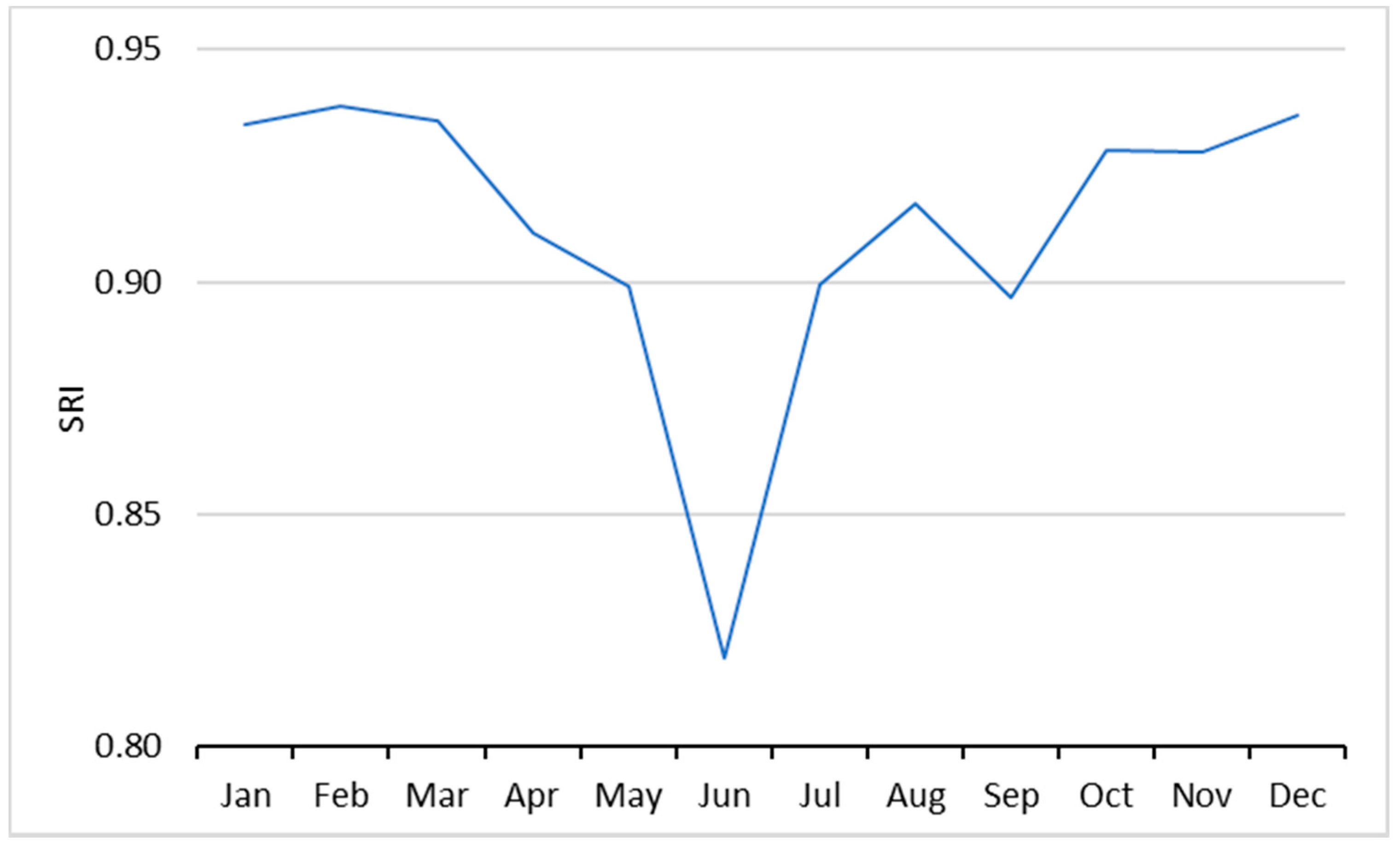
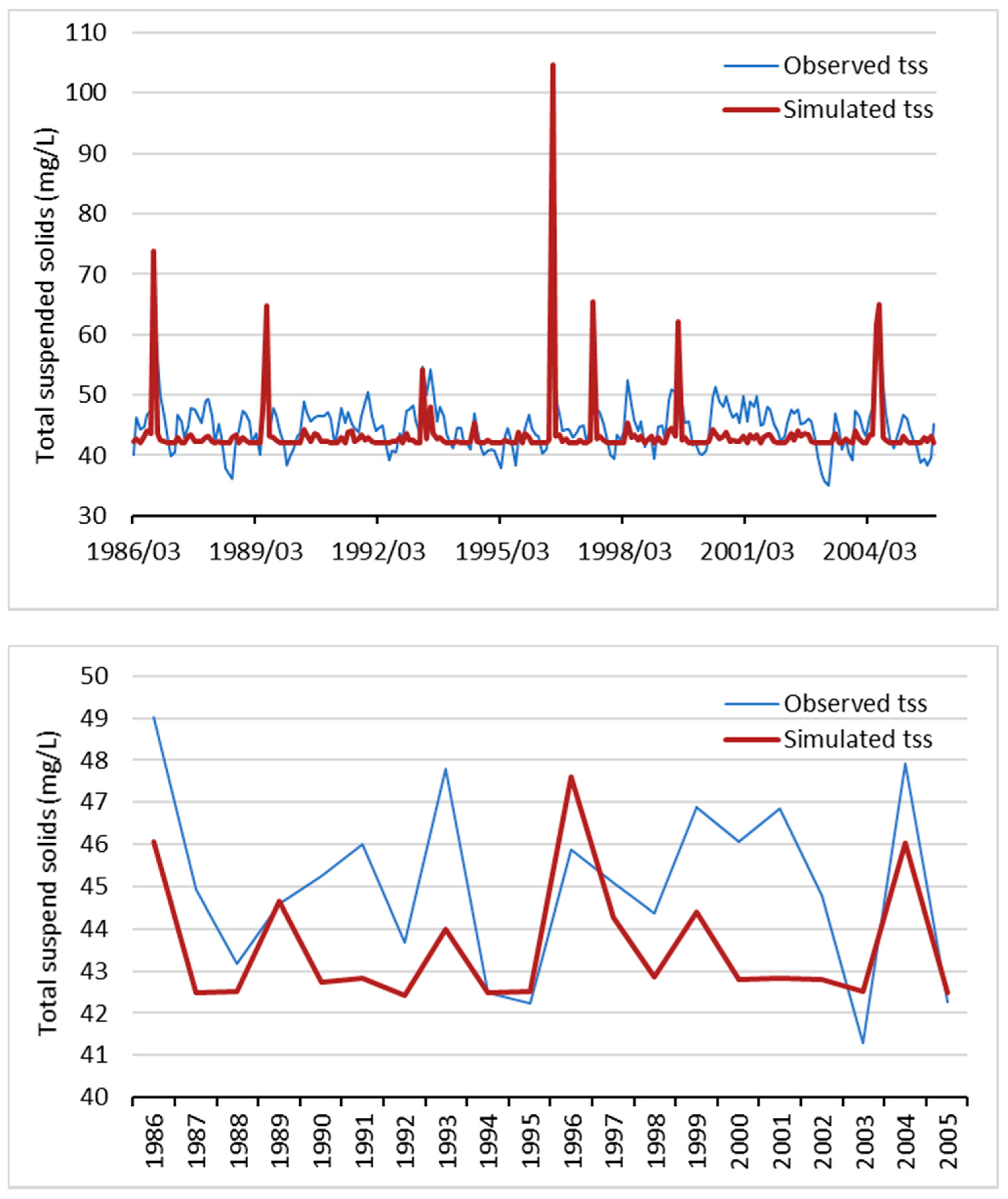
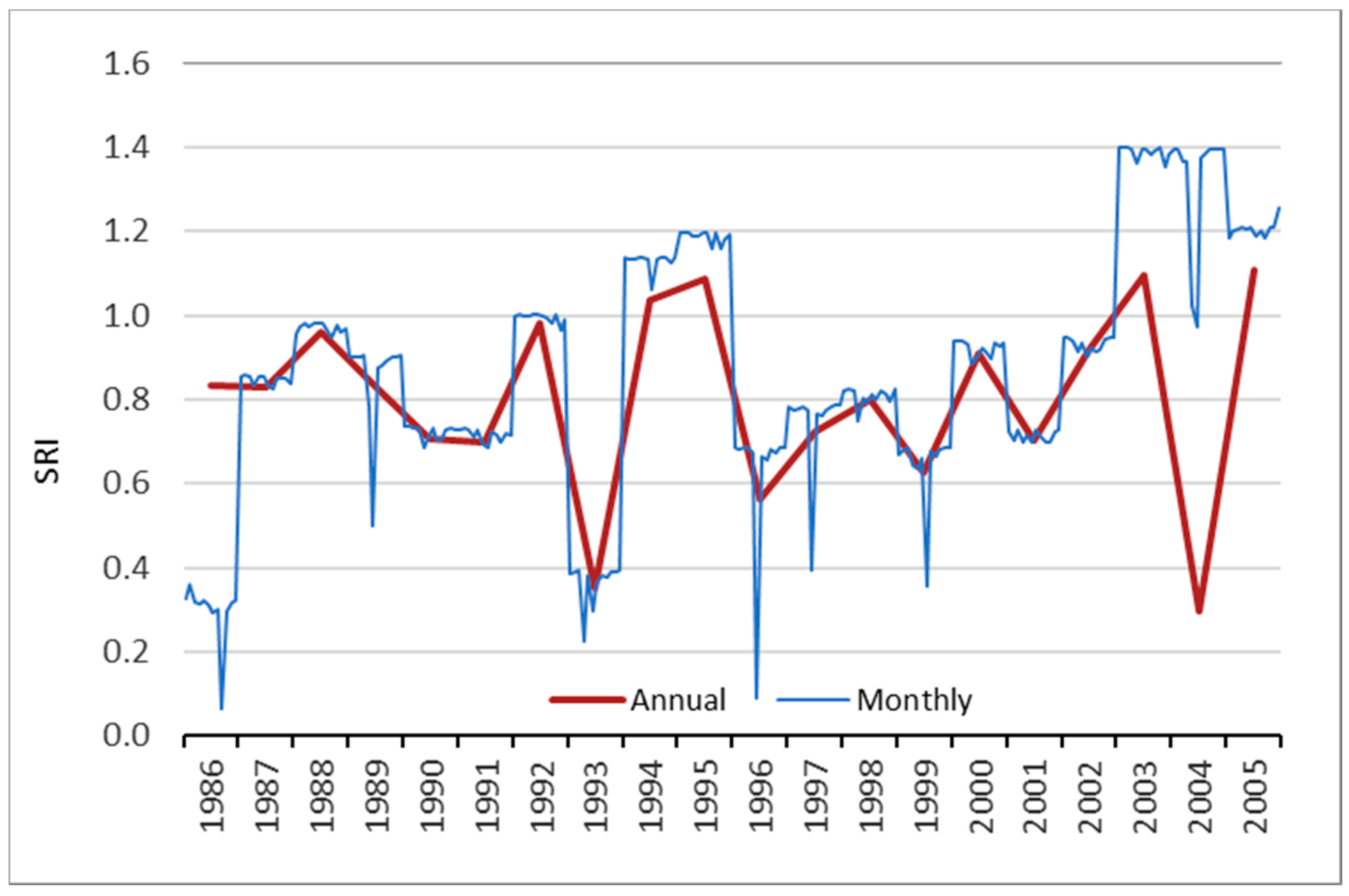
3.2.3. Sediment Regulation Index (SRI)

The monthly and annual time series of SRI are presented in Figure 9, and the mean monthly SRI is presented in Figure 10. As shown in Figure 9, the annual SRI generally fluctuates around 0.8 with a fairly wide range (above 1.1 and below 0.4). The monthly SRI shows similar fluctuations with a larger variability. Although some years (e.g., 1986, 1989, 1996, and 1997) have very low monthly values, their annual SRI is rather high, and for the year 2004, the monthly values are very high, whereas the annual SRI value is low. Based on these findings, it should be noted by decision makers that, with monthly results of SRI, some months of high demand of regulation would be found in low demand years. It suggests that they should plan and apply sediment regulations with more detailed time steps than annual.

The mean monthly SRI in Figure 10 reveals that the SRI is lowest in June. However, spring is the season with the most precipitation. This indicates that the highest sediment regulation demand did not come with the largest precipitation, and it also was associated with temporal soil erodibility variation [38]. The counts of monthly SRI in

Table 4. Counts of sediment regulation index numbers above the mean by one standard deviation or more (A), within one standard deviation from the mean (B), and below the mean by one standard deviation or more (C).

	Category	A	B	C
Month
Jan		2	14	4
Feb		2	14	4
Mar		2	14	4
Apr		2	14	4
May		2	15	3
Jun		5	12	3
Jul		3	13	4
Aug		2	15	3
Sep		2	14	4
Oct		2	14	4
Nov		2	14	4
Dec		2	14	4

as described in Section 2.2.3 show that the further the month is away from June, the fewer the counts of A are, which means less regulation is needed. Along with Figure 10, these monthly results indicate more regulation is needed in summer than the rest of the year.

4. Conclusions

In this paper, a conceptual modeling framework that can simulate ES with fine resolutions was built to conduct ES studies with fine temporal resolutions. The framework includes both a hydrologic model and an ES model. This framework can preprocess and access the input data efficiently and can simulate hydrologic ES at the same temporal resolution as the hydrologic model used in this study. With this framework, hydrologic results were converted to indices results for evaluating water provision, flood control, and sediment regulation in different ways, such as a general increasing or decreasing trend, detailed analysis of the changes, and seasonal changes to be used by decision makers. The results of the three hydrologic ES at both annual and monthly resolutions reveal that annual results alone in ES simulation and analysis for management plans is not adequate for time-sensitive plans, and including fine temporal resolutions is necessary for some ES that are event-based or have large seasonal variations.

The design of the framework established a strategy for the integration of data development, hydrologic and ES modeling, and output analysis supported by national data products for multiple research purposes. The framework established in this study not only confirmed the necessity of the function to study the hydrologic ES with fine temporal resolutions, but also created a workflow for combining different types of ES and hydrologic models for various hydrologic ES-related research. With the organization of tools in a procedural framework, the processes of ES modeling are very straightforward and can be used to set up new ES modeling in any basin in the U.S. for studies similar to the study area in this paper. For other study areas where hydrologic research has already been conducted, only ES data preparation and ES modeling execution would be needed for ES modeling. Additionally, thanks to the flexibility of the framework, other hydrologic models with different mechanisms, other types of ES models, and different climate or land use/cover scenarios could be used in this framework.

References

1. De Groot, R.S.; Alkemade, R.; Braat, L.; Hein, L.; Willemen, L. Challenges in integrating the concept of ecosystem services and values in landscape planning, management and decision making. Ecol. Complex. 2010, 7, 260–272. [Google Scholar] [CrossRef]
2. Millennium Ecosystem Assessment. Ecosystems and Human Well-being: Biodiversity Synthesis; World Resources Institute: Washington, DC, USA, 2005. [Google Scholar]
3. Bagstad, K.J.; Semmens, D.J.; Waage, S.; Winthrop, R. A comparative assessment of decision-support tools for Ecosystem services quantification and valuation. Ecosyst. Serv. 2013, 5, e27–e39. [Google Scholar] [CrossRef]
4. Nelson, E.; Mendoza, G.; Regetz, J.; Polasky, S.; Tallis, H.; Cameron, D.; Chan, K.; Daily, G.; Goldstein, J.; Kareiva, P.; et al. Modeling multiple Ecosystem Services, biodiversity conservation, commodity production, and tradeoffs at landscape scales. Front. Ecol. Environ. 2009, 7, 4–11. [Google Scholar] [CrossRef]
5. Guswa, A.J.; Brauman, K.A.; Brown, C.; Hamel, P.; Keeler, B.L.; Sayre, S.S. Ecosystem Services: Challenges and opportunities for hydrologic modeling to support decision making. Water Resour. Res. 2014, 50, 4535–4544. [Google Scholar] [CrossRef]
6. Bhatt, G.; Kumar, M.; Duffy, C.J. A tightly coupled GIS and distributed hydrologic modeling framework. Environ. Model. Softw. 2014, 62, 70–84. [Google Scholar] [CrossRef]
7. Tallis, H.; Polasky, S. Mapping and Valuing Ecosystem Services as an Approach for Conservation and Natural-Resource Management. Ann. N. Y. Acad. Sci. 2009, 11621, 265–283. [Google Scholar] [CrossRef] [PubMed]
8. Villa, F.; Bagstad, K.; Johnson, G.; Voigt, B. Scientific instruments for climate change adaptation: Estimating and optimizing the efficiency of ecosystem services provision. Economia Agraria y Recursos Naturales 2011, 11, 54–71. [Google Scholar]
9. Zhang, Y.; Claus, H.; Yuan, X. Scale-dependent ecosystem service. In Ecosystem Services in Agricultural and Urban Landscapes; Wratten, S., Sandhu, H., Cullen, R., Costanza, R., Eds.; Wiley-Blackwell: Hoboken, NJ, USA, 2013; pp. 107–121. [Google Scholar]
10. Scholes, R.J.; Reyers, B.; Bigg, R.; Spierenburg, M.J.; Duriappah, A. Multi-scale and cross-scale assessments of scoio-ecological systems and their Ecosystem Services. Curr. Opin. Environ. Sust. 2013, 5, 16–25. [Google Scholar] [CrossRef]
11. Koch, E.W.; Barbier, E.B.; Silliman, B.R.; Reed, D.J.; Perillo, G.M.; Hacker, S.D.; Granek, E.F.; Primavera, J.H.; Muthiga, N.; Polasky, S.; et al. Non-linearity in Ecosystem Services: Temporal and spatial variability in coastal protection. Front. Ecol. Environ. 2009, 7, 29–37. [Google Scholar] [CrossRef]
12. Cline, J.C.; Lorenz, J.J.; Swain, E.D. Linking Hydrologic Modeling and Ecologic Modeling: An Application of Adaptive Ecosystem Management in the Everglades Mangrove Zone of Florida Bay. In Proceedings of the International Environmental Modelling and Software Society iEMSs 2004 International Conference, Osnabrück, Germany, 14–17 June 2004. [Google Scholar]
13. Wlotzka, M.; Haas, E.; Kraft, P.; Heuveline, V.; Klatt, S.; Kraus, D.; Breuer, L. Dynamic Simulation of Land Management Effects on Soil N2O Emissions using a coupled Hydrology-Ecosystem Model. Available online: https://journals.ub.uni-heidelberg.de/index.php/emcl-pp/article/view/11824 (accessed on 31 January 2018).
14. Leh, M.D.K.; Matlock, M.D.; Cummings, E.C.; Nalley, L.L. Quantifying and mapping multiple ecosystem services change in West Africa. Agric. Ecosyst. Environ. 2013, 165, 6–18. [Google Scholar] [CrossRef]
15. Gao, J.; Li, F.; Gao, H.; Zhou, C.; Zhang, X. The impact of land-use change on water-related ecosystem services: A study of the Guishui River Basin, Beijing, China. J. Clean. Prod. 2017, 163, S148–S155. [Google Scholar] [CrossRef]
16. Samal, N.; Wollheim, W.; Zuidema, S.; Stewart, R.; Zhou, Z.; Mineau, M.; Huber, M. A coupled terrestrial and aquatic biogeophysical model of the Upper Merrimack River watershed, New Hampshire, to inform ecosystem services evaluation and management under climate and land-cover change. Ecol. Soc. 2017, 22, 18. [Google Scholar] [CrossRef]
17. Yang, L.; Zhang, L.; Li, Y.; Wu, S. Water-related ecosystem services provided by urban green space: A case study in Yixing City (China). Landsc. Urban Plan. 2015, 136, 40–51. [Google Scholar] [CrossRef]
18. Bai, Y.; Zheng, H.; Ouyang, Z.; Zhuang, C.; Jiang, B. Modeling hydrological ecosystem services and tradeoffs: A case study in Baiyangdian watershed, China. Environ. Earth Sci. 2013, 70, 709–718. [Google Scholar] [CrossRef]
19. Notter, B.; Hurni, H.; Wiesmann, U.; Abbaspour, K. Modelling water provision as an ecosystem service in a large East African river basin. Hydrol. Earth Syst. Sci. 2012, 16, 69. [Google Scholar] [CrossRef]
20. Schmalz, B.; Kruse, M.; Kiesel, J.; Müller, F.; Fohrer, N. Water-related ecosystem services in Western Siberian lowland basins—Analysing and mapping spatial and seasonal effects on regulating services based on ecohydrological modelling results. Ecol. Indic. 2016, 71, 55–65. [Google Scholar] [CrossRef]
21. Logsdon, R.A.; Chaubey, I. A quantitative approach to evaluating ecosystem services. Ecol. Model. 2013, 257, 57–65. [Google Scholar] [CrossRef]
22. Duda, P.B.; Hummel, P.R.; Donigian, A.S., Jr.; Iimhoff, J.C. BASINS/HSPF Model Use, Calibration and Validation. Trans. ASABE 2012, 55, 1523–1547. [Google Scholar] [CrossRef]
23. National Exposure Research Laboratory (U.S.). Hydrological simulation program--FORTRAN user’s manual for version 11. Available online: http://purl.access.gpo.gov/GPO/LPS35019 (accessed on 31 January 2018).
24. Alarcon, V.J.; Mcanally, W.; Diaz-Ramirez, J.; Martin, J.; Cartwright, J. A Hydrological Model of the Mobile River Watershed, Southeastern USA. AIP Conf. Proc. 2009, 1148, 641–645. [Google Scholar]
25. Hsu, S.M.; Chiou, L.B.; Lin, G.F.; Chao, C.H.; Wen, H.Y.; Ku, C.Y. Applications of simulation technique on debris-flow hazard zone delineation: A case study in hualien county, taiwan. Nat. Hazards Earth Syst. Sci. 2010, 10, 535–545. [Google Scholar] [CrossRef]
26. Chen, J.; Theller, L.; Gitau, M.W.; Engel, B.A.; Harbor, J.M. Urbanization impacts on surface runoff of the contiguous United States. J. Environ. Manag. 2017, 187, 470–481. [Google Scholar] [CrossRef] [PubMed]
27. Hayashi, S.; Murakami, S.; Xu, K.; Watanabe, M.; Xu, B. Daily runoff simulation by an integrated catchment model in the middle and lower regions of the changjiang basin, china. J. Hydrol. Eng. 2008, 13, 846–862. [Google Scholar] [CrossRef]
28. Tzoraki, O.; Nikolaidis, N.P. A generalized framework for modeling the hydrologic and biogeochemical response of a Mediterranean temporary river basin. J. Hydrol. 2007, 346, 112–121. [Google Scholar] [CrossRef]
29. Choi, W.; Pan, F.; Wu, C. Impacts of climate change and urban growth on the streamflow of the Milwaukee River (Wisconsin, USA). Reg. Environ. Chang. 2017, 17, 889–899. [Google Scholar] [CrossRef]
30. U.S. Geological Survey. USGS National Elevation Dataset (NED) 1 arc-second Downloadable Data Collection from The National Map 3D Elevation Program (3DEP)—National Geospatial Data Asset (NGDA) National Elevation Data Set (NED): U.S. Geological Survey; U.S. Geological Survey: Reston, VA, USA, 2016.
31. Vogelmann, J.E. Completion of the 1990s national land cover data set for the conterminous United States from Landsat thematic mapper data and ancillary data sources. Photogramm. Eng. Remote Sens. 2001, 67, 650–655. [Google Scholar]
32. Serbin, S.P.; Kucharik, C.J. Spatiotemporal mapping of temperature and precipitation for the development of a multidecadal climatic dataset for Wisconsin. J. Appl. Meteorol. Climatol. 2009, 48, 742–757. [Google Scholar] [CrossRef]
33. U.S. Geological Survey. National Water Information System data available on the World Wide Web (USGS Water Data for the Nation). 2016. Available online: http://waterdata.usgs.gov/nwis/ (accessed on 10 June 2012).
34. Tennant, D.L. Instream flow regimens for fish, wildlife, recreation and related environmental resources. Fisheries 1976, 1, 6–10. [Google Scholar] [CrossRef]
35. De Guenni, L.B.; Cardoso, M.; Goldammer, J.; Hurtt, G.; Mata, L.J.; Ebi, K.; House, J.; Valdes, J. Regulation of natural hazards: Floods and fires. In Ecosystems and Human Well-being: Current State and Trends; Norgaard, R., Ed.; Island Press: Washington, DC, USA, 2005. [Google Scholar]
36. Soil Survey Staff, Natural Resources Conservation Service, United States Department of Agriculture. Web Soil Survey. Available online: http://websoilsurvey.nrcs.usda.gov/ (accessed on 25 September 2018).
37. Wisconsin. Department Of Natural Resources. The state of the Milwaukee River Basin. Available online: https://lccn.loc.gov/2002418368 (accessed on 31 January 2018).
38. Bajracharya, R.M.; Lal, R. Seasonal Soil Loss and Erodibility Variation on a Miamian Silt Loam Soil. (Soil and Water Management and Conservation). Soil Sci. Soc. Am. J. 1992, 56, 1560. [Google Scholar] [CrossRef]
Figure 1. Workflow of the modeling framework.
Hydrology 06 00014 g001
Figure 2. Study area: Milwaukee River basin boundary, subbasins delineated for hydrological modeling, streamflow measurement sites, elevation, climate data grids, and stream network.
Hydrology 06 00014 g002
Figure 3. Hydrologic time series for calibration and validation periods at the USGS streamflow measurement site Milwaukee River at Milwaukee, WI (04087000).
Hydrology 06 00014 g003
Figure 4. Total suspended solids as monthly (top) and annual (bottom) time series between simulation and observation.
Hydrology 06 00014 g004
Figure 5. Annual and monthly water provision index time series. WPI: water provision index.
Hydrology 06 00014 g005
Figure 6. Mean monthly water provision index.
Hydrology 06 00014 g006
Figure 7. Annual and monthly flood regulation index time series. FRI: flood regulation index.
Hydrology 06 00014 g007
Figure 8. Mean monthly flood regulation index.
Hydrology 06 00014 g008
Figure 9. Annual and monthly sediment regulation index time series. SRI: sediment regulation index.
Hydrology 06 00014 g009
Figure 10. Mean monthly sediment regulation index.
Hydrology 06 00014 g010