Evaluating Remote Sensing Model Specification Methods for Estimating Water Quality in Optically Diverse Lakes throughout the Growing Season

Abstract

Spectral images from remote sensing platforms are extensively used to estimate chlorophyll-a (chl-a) concentrations for water quality studies. Empirical models used for estimation are often based on physical principles related to light absorption and emission properties of chl-a and generally relying on spectral bands in the green, blue, and near-infrared bands. Because the physical characteristics, constituents, and algae populations vary widely from lake to lake, it can be difficult to estimate coefficients for these models. Many studies select a model form that is a function of these bands, determine model coefficients by correlating remotely-measured surface reflectance data and coincidentally measured in-situ chl-a concentrations, and then apply the model to estimate chl-a concentrations for the entire water body. Recent work has demonstrated an alternative approach using simple statistical learning methods (Multiple Linear Stepwise Regression (MLSR)) which uses historical, non-coincident field data to develop sub-seasonal remote sensing chl-a models. We extend this previous work by comparing this method against models from literature, and explore model performance for a region of lakes in Central Utah with varying optical complexity, including two relatively clear intermountain reservoirs (Deer Creek and Jordanelle) and a highly turbid, shallow lake (Utah Lake). This study evaluates the suitability of these different methods for model parameterization for this area and whether a sub-seasonal approach improves performance of standard model forms from literature. We found that while some of the common spectral bands used in literature are selected by the data-driven MLSR method for the lakes in the study region, there are also other spectral bands and band interactions that are often more significant for these lakes. Comparison of model fit shows an improvement in model fit using the data-driven parameterization method over the more traditional physics-based modeling approaches from literature. This suggests that the sub-seasonal approach and exploitation of information contained in other bands helps account for lake-specific optical characteristics, such as suspended solids and other constituents contributing to water color, as well as unique (and season-specific) algae populations, which contribute to the spectral signature of the lake surface, rather than only relying on a generalized optical signature of chl-a. Consideration of these other bands is important for development of models for long-term and entire growing season applications in optically diverse water bodies.

1. Introduction

1.1. Background

Water quality studies that use remote sensing data provide complete spatial coverage of lakes and reservoirs and can identify valuable spatial information not apparent from point samples. However, model parameterization can be a major challenge. This paper investigates simple approaches for seasonally segmenting models and using machine learning methods to address this issue. A wide variety of methods have been used to develop models that exploit remotely sensed reflectance data to estimate water quality constituents, including concentrations of surface chlorophyll-a (chl-a), which are often used as a proxy or indicator for algae biomass [1]. Chl-a is essential for photosynthesis, and is found in all species of algae (including phytoplankton and photosynthesizing cyanobacteria). For empirical modeling approaches, many published remote sensing studies use relationships between field samples of chl-a and associated pixels in satellite images to estimate in-lake conditions. These models are then used to estimate chl-a concentrations for the remaining surface water pixels in the satellite image, and in some cases, are applied to other images in the satellite record to establish long histories. This provides valuable temporal information by extending and supplementing field records which are often limited or irregular. While empirical chl-a models are frequently used for long-term water quality evaluations and the products from these evaluations are valuable, there are a number of considerations for development and application at the regional level, especially when evaluating lakes and reservoirs with diverse optical characteristics.

Lake chl-a studies in literature vary widely in approach for model development and application/scope. Because of the requirement for field samples for calibrating the empirical models, many previous studies have focused on a small portion of the growing season when potentially toxic algae (cyanobacteria) are at a maximum (usually in mid to late summer) [2]. However, high chl-a concentrations and algae blooms can occur earlier in the growing season. As major bloom events are an increasing concern, it has become increasingly important to utilize data from throughout the growing season data to better understand bloom dynamics such as timing and preceding conditions. Recent studies have demonstrated the technique of splitting the growing season and developing unique models for each sub-season to reflect population succession of algae (with different species of algae dominating at different times in the growing season). These sub-seasonal models performed better than models developed only using late season data for calibration [3,4,5]. With respect to scope, some studies limit the application of the developed model to images with coincident ground truth (i.e., field samples) [6,7,8]. This approach does not exploit potential remote sensing benefits such as high frequency or long time-histories of data [9]. A growing number of studies, however, apply calibrated models to all available imagery which greatly enhances the temporal record [10,11,12]. When applying a model to all historical imagery, it may increase model accuracy if differences in the seasonal algae populations are represented (e.g., through sub-seasonal models).

In addition to these empirical modeling methods, the selection of remote sensing data also varies in literature. A variety of remote sensing instruments (Landsat, MODIS (Moderate Resolution Imaging Spectroradiometer), MERIS (MEdium Resolution Imaging Spectrometer), Sentinel, etc.) have been used in previous long-term remote sensing studies [13], each of which has tradeoffs of spectral and temporal resolution and temporal extent. Despite its shortcomings in spectral resolution and time between image acquisition, Landsat is one of the most commonly used satellite instruments for long-term studies. Landsat (from Landsat 5 Thematic Mapper-on) provides an extensive historical record with imagery from 1984 to the present. The temporal resolution of this remotely sensed imagery (every 16 days) is often much better compared to field sampling records, which may be irregular or infrequent, and the spatial resolution (30 m) is generally sufficient for capturing spatial variability in surface conditions [14]. Another aspect of data selection is the matching of remotely sensed data with field-sampled, ground-truth data. While a coincidental sample and image provides the optimal data for model development as both data sets (field-sampled and remotely sensed data) measure the same conditions, many studies of surface water conditions (quality and clarity) rely on near-coincident data simply because of insufficient matches between field samples and remotely sensed imagery [12,15,16,17].

Previous studies have also used a wide variety of chl-a detection algorithms [13] and model parameterization techniques. Models to estimate chl-a concentrations are often physics-based, that is they rely on the optical properties of chl-a and correlate the measured reflectance spectra to expected chl-a behaviors [18]. Early work on estimating chl-a concentrations used spectral irradiance reflection, which is the ratio of spectral upwelling to spectral downwelling [19,20]:

$$R\left(z,\lambda \right)=\frac{E_u\left(z,\lambda \right)}{E_d\left(z,\lambda \right)},$$

(1)

where R(z, λ) is the spectral irradiance reflectance or irradiance ratio, z is the depth within the water column or air above the water surface, λ is wave length, E_u is the upwelling reflectance, and E_d is the downwelling spectral reflectance. Most recent work uses remote-sensing reflectance R_rs which is also a ratio of spectral upwelling to downwelling but “in air”, meaning it is evaluated just above the water surface, that is the data measured at the sensor (satellite) is corrected for the intervening atmosphere to estimate the measurement at the surface [21,22].

$$R_{rs}\left(\theta ,\varphi ,\lambda \right)=\frac{L_w\left(in air, \theta ,\varphi ,\lambda \right)}{E_d\left(in air,\lambda \right)} \left(s{r}^{-1}\right),$$

(2)

Here, “in air” means that R_rs uses the water-leaving radiance, L_w, and the downwelling, E_d, just above the water surface. This is a measure of how much of the downwelling radiance incident on the water surface at angle, θ, is reflected in a direction measured as (θ, ϕ), this is usually calculated assuming a nadir viewing direction only, though most data in a scene are off-nadir. R_rs is less sensitive to environmental conditions such as sun angle or atmospheric conditions as conditions are computed at the water surface based on satellite measurements [23,24].

Once the data have been corrected to surface reflectance, models are typically created using known absorbance and fluorescence properties of chl-a. General algae spectral characteristics include: a peak near 550–600 nm, a minimum near 670 nm, and a peak at 700 nm. These features can be used to identify chl-a concentrations with hyper-spectral instruments using spectral matching approaches [8,25,26,27,28] and empirical methods [29]. However, the spectral resolution of some remote sensing instruments, including Landsat, is relatively coarse, and therefore does not support chl-a identification by spectral matching [15]. The difficulty in capturing these known spectral features has led to a broad range of empirical lake-specific relationships which have been used extensively to estimate chl-a concentration [8,12,13,30,31,32]. Most of these empirical models use Landsat reflectance data from the first 4 bands as these are the spectral regions with defining chl-a features. The bands most commonly reported in the literature are Band-1 and Band-3, bands related to blue and red colors, respectively, though it is common to use other combinations or bands [33]. Many remote sensing methods to estimate chl-a concentrations only use satellite bands associated with the absorption properties of chl-a. Matthews [13] provides a thorough overview of the variety of bands chosen for chl-a detection. Some modelers have selected several of these standard forms, determined model coefficients using a linear regression approach, compared error metrics or performance against other remotely sensed products among the selected models, and then used the best model to estimate chl-a concentrations or other measures of algal blooms throughout the lake [34].

1.2. Goals and Objectives

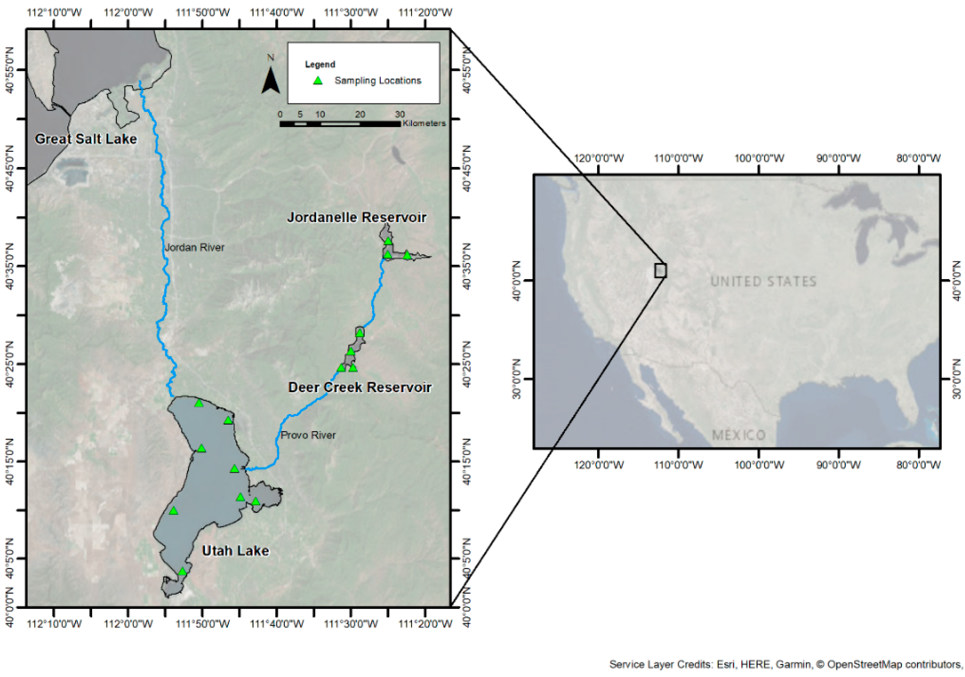
Our primary objective is to explore approaches for parameterization and calibration of empirical chl-a models that are suitable for long-term applications (i.e., throughout the growing season, using out-of-sample imagery). The approaches that we compare include: multiple linear regression (MLR) to calibrate algorithms based on standard forms for Landsat applications in other freshwater regions, and a data-driven, statistical learning method (multiple linear stepwise regression (MLSR)) that considers all possible spectral bands and band ratios.

We build on previous work that compares Landsat algorithms from the literature [11,35] by evaluating lake-specific, sub-seasonal parameterization methods and their ability to reflect the unique optical properties of individual bodies of water throughout the growing season. These unique properties include characteristics of the lake or reservoir (e.g., other constituents, bottom reflectance) and properties of the algae (e.g., seasonal-specific speciation), which have the potential to contribute to the optical signature of the surface water.

We present and compare methods for using simple MLR and MLSR for developing and applying empirical chl-a models within a case study for several lakes in north-central Utah: Deer Creek and Jordanelle reservoirs and Utah Lake. These modeling approaches use an historical, near-coincident dataset of field and Landsat 5 and 7 data. Through this case study, we showcase differences in the performance of different algorithms, and evaluate how standard forms that perform well in one region translate to the study area and how performance can differ within a region where there are distinct algae populations and physical/optical characteristics.

2. Study Area

2.1. Case Study Locations

The region of the case study contains a closely connected series of reservoirs and a major lake in north-central Utah. The two reservoirs are located upstream of Utah Lake, and are key components in the water supply system for the greater Salt Lake City–Provo metropolitan area, and algae blooms can pose a threat to these drinking water sources and popular recreational sites. Utah Lake has received national and global attention because of its long history with concerns over algae bloom, especially in recent years, as massive toxic blooms have caused public health concerns and areas of the lake have been restricted to recreationists [36]. We selected Deer Creek and Jordanelle Reservoirs and Utah Lake for this case study because of the availability of relatively long-term historical data and consistency in field sampling techniques within each lake. Algae (through chl-a concentrations) have been regularly monitored in Deer Creek reservoir since the early 1984 and in the upstream Jordanelle reservoir since 1993 (when it was built), as part of mitigation efforts to address high levels of phosphorus and algal biomass [37]. Deer Creek and Jordanelle reservoirs are similar in physical characteristics and elevation, and are close enough to be in a single Landsat image. Deer Creek reservoir is downstream from Jordanelle and in the same watershed. Flows from Deer Creek reservoir and the Provo River are the single biggest point-source input to Utah Lake, which is located southwest of Deer Creek in Utah County. This lake differs greatly from the two reservoirs in its size, elevation, and amount of development/types of inputs. The color and clarity of Utah Lake also make this highly unique; its shallow nature makes it highly susceptible to sediment suspension (from bottom-feeding carp and mixing due to recreation and weather events), and the lake often appears “milky” due to high levels of calcium precipitates. This lake also has been the focus of historical sampling, with a record from 1995-present of surface chl-a and other water quality parameters. During this time, turbidity has averaged approximately 95 NTU. These reservoirs are closely connected to the Great Salt Lake, which receives outflow from Utah Lake via the Jordan River and through surface water exchanges and aqueducts from Deer Creek to the Salt Lake City area.

Figure 1 shows an overview of the study area and locations where field data were collected.

2.2. Deer Creek Reservoir

Deer Creek is located in the Wasatch Mountains on the Provo River. It supplies potable water for much of the Salt Lake City valley. The reservoir has a surface area of 1200 hectares (2965 acres), with an approximate capacity of 240 million cubic meters (193,600 acre-feet) and maximum depth of 42 m (137 feet) near the dam [38]. In addition to recreational use, agriculture and potable water supply accounts for 38% and 62% of water use, respectively. Potable use is expected to increase as the area continues to develop. Deer Creek Reservoir was identified as highly eutrophic in the 1970s and 1980s, and continues to exhibit high phosphorus and low dissolved oxygen levels during the summer.

2.3. Jordanelle Reservoir

Jordanelle is a large reservoir with a surface area of about 1335 hectares (3300 acres) and feeds into Deer Creek Reservoir. It has a capacity of approximately 445 million cubic meters (360,500 acre-feet), and a maximum depth of 89 m (292 feet) [37]. The dam was completed and the reservoir completely filled in 1994. It is used for a wide range of purposes including recreation, irrigation, industrial, and potable water supply.

2.4. Utah Lake

Utah Lake a shallow lake with an average depth of approximately 2.74 m, and has higher salinity levels than most freshwater lakes (around 0.1%) which fluctuate depending on inflows and evaporation [39]. Surrounding Utah Lake, there are numerous campgrounds, public access points and marinas, supporting a variety of recreational activity. The lake supports a large migratory bird population, and is heavily monitored because it is a habitat for the endangered June sucker (Chasmistes liorus) species. It also provides massive economic value by serving as a receiving body for treated wastewater from the nearby urban area that lies to the north, east, and south of the lake.

3. Methodology and Data

3.1. Data

For this study we used field data from Deer Creek and Jordanelle reservoirs collected by the Central Utah Water Conservancy District (CUWCD) that were analyzed for chl-a concentration. We used images from the Landsat-5 Thematic Mapper (TM) from 1984–1999 and Landsat-7 Enhanced Thematic Mapper Plus (ETM+) from 1999–2012.

Deer Creek and Jordanelle Reservoir field data were collected monthly at several locations in each reservoir (Figure 1). We used data from both reservoirs, which have similar physical characteristics, to develop one set of sub-seasonal models as opposed to developing reservoir-specific models. For the reservoir models, we developed three sub-seasonal models: early-season (April through May), mid-season (June through July), and late-season (August through September). We used two sub-seasons for Utah Lake, May-June, and July-September. These seasons were selected based on general observed reservoir conditions, suggestions by reservoir managers [40] and documented speciation [41,42].

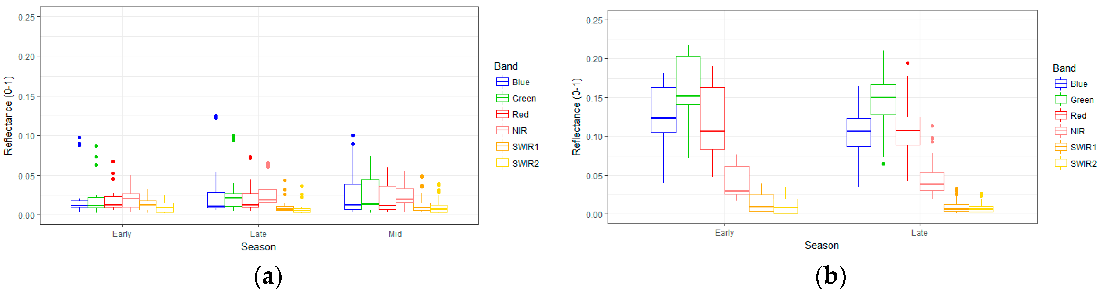
3.2. Data Preparation

3.2.1. Field Data

Field samples of surface chl-a for Deer Creek were available over the period from 1984–2013, and field samples from Jordenelle were available over a period from 1993–2012, collected by the CUWCD. The CUWCD, as a government body, provides annual reports that present the data and methods used. We used only field samples taken within two meters of the surface to represent surface chl-a concentrations to compute correlation with Landsat-measured surface reflectance. Data for Utah Lake were obtained from the Utah Division of Water Quality (UDWQ), and consist of surface chl-a (uncorrected for accessory pigments), collected within one meter from the surface, from 1995–2011.

3.2.2. Landsat Data

Remotely-sensed data for Utah Lake were obtained from Landsat surface reflectance products using Google Earth Engine [43]. The Landsat surface reflectance products available through Earth Engine are produced by the United States Geological Survey (USGS), and are generated using the Landsat Ecosystem Disturbance Adaptive Processing System (LEDAPS) [44], which converts the top of atmosphere (TOA) reflectance to surface reflectance.

Data for Jordanelle and Deer Creek had been collected prior to the release of Google Earth Engine, so images were calibrated for top of the atmosphere reflectance in the range of 0–1 using ENVI Version 4.7 (Exelis Visual Information Solutions, Boulder, Colorado) software internal procedures based on the following equation:

$${\rho }_{\lambda }=\frac{\pi L_{\lambda }{d}^2}{S_{\lambda }\sin \theta },$$

(3)

where L_λ is radiance in units of W/(m² sr µm) measured by the sensor, d is the earth to sun distance in astronomical units, S_λ is the solar irradiance in units of W/(m² µm), and θ is the sun elevation in degrees. Atmospheric correction (dark-object subtraction method) was then applied to remove effects from the atmosphere (i.e., aerosols, water vapor) and approximate surface reflectance.

For each field sampling location (Figure 1) we created a corresponding Landsat reflectance spectrum using the filtered mean of each band using a 3 × 3-pixel grid surrounding the field site. This filtered nine-pixel grid was used to reduce noise and to address the spatial uncertainty in the field sampling locations [45]. The mean value for each band was computed as:

$$\mathrm{Filtered}\mathrm{Mean}=\frac{{\mathsf{\Sigma }}_i\left(1.5\ast \sigma -\overline{X}\right)<X_i<\left(1.5\ast \sigma +\overline{X}\right)}{N},$$

(4)

where $\overline{X}$ = unfiltered mean, $\sigma$ = unfiltered standard deviation, and $N$ = number of values within ± 1.5. This method helps eliminate the influence of noisy data [45]. For this study, differences in retrieving and processing reflectance data are ignored by developing distinct models for the reservoirs and lake. Figure 2 shows the range of reflectance values for the lake and reservoirs.

The range of reflectance values within the study area highlight how distinct the lake is from the reservoirs, with much greater reflectance in the visible range. Additionally, there are differences in the spectral signatures between sub-seasons.

3.2.3. Field and Satellite Data Pairs

Historical field data in the reservoirs and Utah Lake were not collected for the purpose of calibrating remote sensing models, so the number of samples with coincident satellite overpasses is limited. Previous studies that develop empirical models of lake surface conditions (water quality and clarity) with limited historical data have used time-windows from ±24 h [17] up to ±10 days [12] for near-coincident data. Because of the limited number of exact matches in the study area, we used field data taken on the same day, but not coincident with a satellite overpass for early- and late-season models for the reservoirs, and within 24 h of a satellite overpass for the mid-season reservoir model and both the early and late-season model for Utah Lake. The difference in field sampling and satellite overpass is a source of potential error in the models, as surface conditions could be affected by hydrodynamic processes and mixing influences from local environmental factors (e.g., wind) or recreation. Previous high-frequency (daily) sampling in Utah Lake supports the use of a relatively short time-window because of the distinct drop in autocorrelation for most sites in Utah Lake after 2 days [14].

The resulting pairs of satellite data and field samples are summarized for the seasons and lakes in

Table 1. Summary of pairs of remotely sensed data and field-measured surface Chl-a during the entire Historical Sampling Period.

Lake	Season	Time-Window	Number of Pairs	Range and Average Field-Sampled Chl-a (µg/L) during Historical Sampling Period	Range and Average Field-Sampled Chl-a (µg/L) from Paired Samples
Utah Lake	Early	±24 h	10	0.8–45; 7.6	1.2–45; 9.4
	Late	±24 h	46	0.2–324.9; 38.3	0.2–185.5; 27.1
Deer Creek and Jordanelle Reservoirs	Early	Same day	18	0.2–35.4; 6.9	0.2–6.3; 3.2
	Mid	±24 h	42	0.2–21.3; 4.3	0.2–21.3; 6.3
	Late	Same day	25	0.1–196; 7.2	0.2–196; 23.2

.

3.3. Multiple Linear Regression on Standard Forms

MLR and MLSR requires that the response variable, chl-a concentration, is normally distributed. We performed a Lilliefors test on the data to determine if our data were normally distributed [46,47]. We found that for all but the early-season reservoir data, chl-a concentrations were not normally distributed, however, their log transforms closely approximated a normal distribution. For these seasons, we used a log transform to generate our models. That is, the response variables were chl-a concentration and the ln(chl-a concentration) for the early season reservoir model, and all other models, respectively.

3.3.1. Overview of MLR and Coefficient Estimation

MLR is a commonly used method and most reported remote sensing models use MLSR to determine appropriate model coefficients. MLR quantifies the relationships between several predictor variables and a response parameter to create a model than estimates the response given the predictors. For remote sensing models, traditionally the scientist chooses a model form and the associated predictor variables (e.g., Landsat bands) then uses MLR to fit the coefficients for the model. For example, Giardino et al. [6] chose a model of the following form:

$$\mathrm{chl}-a={\beta }_1{x}_1+{\beta }_1{x}_1+c$$

(5)

where $x_1$ and $x_2$ are Landsat Thematic Mapper bands 1 (B₁) and 3 (B₃), while ${\beta }_1, {\beta }_2$, and c are the fitted coefficients for the model. They used MLR methods to compute the coefficients resulting in the following equation that they used to estimate chl-a concentrations:

$$\mathrm{chl}-a=11.18B_1-8.96B_2-3.28 \mathrm{mg}/{\mathrm{m}}^3$$

(6)

MLR methods can be extended to include as many predictor variables as are available. The general form of an MLSR model is:

$$y_i={\beta }_1{x}_{i1}+\dots +{\beta }_p{x}_{ip}+{\epsilon }_i,i=1,\dots ,n,$$

(7)

where n is the number of predictor variables.

MLR assumes that the relationship between the response variable, y_i and the regressors (i.e., predictors) x_i is linear and that the response variable is normally distributed. This produces a set of equations that can be readily solved

The MLR equation in matrix form is:

$$\mathit{y}=\mathit{X}\mathit{\beta }+\mathit{\epsilon },$$

(8)

where

$$\mathit{y}=\left\{\begin{array}{c}{y}_1\\ ⋮\\ y_n\end{array}\right\},\mathit{X}=\left\{\begin{array}{ccc}{x}_{11}& \dots & x_{1p}\\ x_{21}& \dots & x_{2p}\\ x_{n1}& \dots & x_{np}\end{array}\right\},\mathit{\beta }=\left\{\begin{array}{c}{\beta }_1\\ ⋮\\ {\beta }_n\end{array}\right\}, and \mathit{\epsilon }=\left\{\begin{array}{c}{\mathit{\epsilon }}_1\\ ⋮\\ {\mathit{\epsilon }}_n\end{array}\right\}$$

(9)

Equation (7) is solved for ${\beta }_i$ by minimizing the sum of the squares of the error term $\mathit{\epsilon }$. This is the source of the “least squares” portion of the name. Using matrix algebra, it can be shown that the least-squares estimate of $\beta$, is:

$$\mathit{\beta }={\left({\mathit{X}}^{\prime }\mathit{X}\right)}^{-\mathbf{1}}{\mathit{X}}^{\prime }\mathit{y}$$

(10)

If the inverse exists, this equation can be solved directly. This inverse of ${\mathit{X}}^{\prime }\mathit{X}$ exists if the columns of $\mathit{X}$ are independent, that is no column is a linear combination of the other columns [46,47]. The solution of Equation (8) provides the coefficients for a predictive model in the form of Equation (5).

MLR assumes linear relationships, however, various studies have documented non-linear relationships between field chl-a concentrations and Landsat-measured reflectance [13]. These studies showed that, while relationships between reflectance and chl-a may not be linear, correlations between chl-a concentrations and various band ratios, such as B₁/B₃, may be linear. Linear correlations may also exist between chl-a concentrations and log band transforms. These transformed variables can then be used in MLR models. Also, as noted, MLR assumes the response variable, chl-a concentration, is normally distributed. Often distributions of chl-a concentrations are log-normal, so a generalized linear model with a log-transform of the chl-a concentration can be used in the MLR model to meet this assumption [5].

3.3.2. Select Algorithms for Evaluation

A review of different Landsat-based algorithms for water quality and clarity (as well as algorithms used with other remote sensing instruments) is detailed in Matthews [13]. A comparison of several of these standard forms, (along with other bands and band combinations not included in this review) was explored in the application to a portion of Lake Erie [11]. We have selected algorithms that are potentially appropriate for the lakes in this study, based on suggested use in the literature, bio-optical theory, and similar characteristics of application regions (i.e., levels of development). For example, some algorithms are recommended for lakes with high chl-a, others were developed and applied in regions with very little development, and others are recommended for waters with high turbidity. The reservoirs and Utah Lake cover a range of these conditions. Some algorithms were excluded because they were developed for water bodies with extremely low chl-a concentrations (e.g., <5 µg/L).

Table 2. Selected Algorithms for Empirical Landsat Chl-a Detection Models and Supporting Studies.

#	Landsat Bands	References and Lake(s) Used for Calibration	Notes
1	B3/B1	Shallow Canadian Lakes [48] 15 MN Lakes [33] Green Bay and Lake Michigan [49]	Recommended for use in high (>20 µg/L) chl-a conditions [13] and highly turbid lakes [49]
2	B3/B4	Lake Kinneret, Israel [8] Lake Chagan, Kazakhstan [50]	Recommended for use in high (>20 µg/L) chl-a conditions [13]
3	(a) B2/B1 (b) Log(B1/B2)	20 European waterbodies [51] a Lake Erken, Sweden [32] b	Recommended for use in low (<20 µg/L) chl-a-a conditions [13]
4	(B1−B3)/B2	Lake Kinneret, Israel [52] Lake Garda, Italy [53]	Accounts for the increased effect of inorganic suspended solids that occurs with decreased chl-a concentrations [13]
5	(a) B1, B2, and B3 (b) B2, B3 (c) B1, B2 (d) Log(B2)	Lake Balaton, Hungary [54] a Beaver Reservoir, Arkansas, USA [55] a Reelfoot Lake, Tennessee, USA [56] b Lake Iseo, Italy [7] c Green Bay and Lake Michigan, Wisconsin, USA [57] d	Specifically used for shallow waters dominated by high levels of suspended sediments
6	(a) B4 (b) B4-B5	Lake Taihu, China [10]	Performs well under high chl-a conditions [58] Based on similar to approaches in ocean color sensing for turbid waters [59,60]

lists the algorithms we selected, along with supporting studies.

For each of these algorithms, we performed an MLR to estimate coefficients, and then evaluate goodness of fit through root-mean square error (RMSE), observed vs. modeled R² values, and Nash-Sutcliffe Efficiency (NSE) [61]. The NSE, was originally developed to assess goodness of fit for hydrological models, however it can also be generally used to evaluate model predictions against observed data. Values of NSE range from −∞ to 1, where 1 is a perfect match between the modeled and observed values. R Statistical Software (Version 3.4.4) was used to perform statistical analysis.

This process was repeated with two variations: (1) single season models specific to either the reservoirs or Utah Lake and (2) sub-seasonal models specific to either the reservoirs or Utah Lake. This was done to evaluate importance of each band (or band interaction) relative to the effects of seasonality and lake-specific characteristics. Preliminary modeling limited to Deer Creek has shown an improvement in sub-seasonal models over single models [3,4,5]. Models using both Deer Creek and Jordanelle data together showed a similar improvement where sub-seasonal models were more accurate in estimating chl-a throughout the growing season than a single model developed using only data from the latter part of the summer [5]. Different algal groups that are present in these reservoirs, (i.e., diatoms, chlorophyta, and blue-green algae), have different visual presentations with respect to chl-a concentrations. Sub-seasonal models account for these differences by recognizing that different algal groups (with differing spectral signatures) are dominant at different times [62,63]. These initial models were developed using general MLSR methods, however, the methods and results were not evaluated with respect to other modeling forms from literature or compared to other lakes with different characteristics.

The resulting models follow Equation (5) where, y_i is the estimated chl-a value at a location i and x_ip are the predictor variables, p, at location i, and ε is the error. As discussed, the data pair y_i and x_ip represent the field data sample and associated Landsat pixel reflectance values.

3.4. Statistical Learning–Multiple Linear Stepwise Regression

Overview of MLSR

Step-wise regression analysis creates multi-linear regression models by systematically selecting the predictor parameters used in the resulting equation [45]. MLSR is a common statistical learning technique used to explore different possibilities for model specification. An overview of the method can be found in texts such as [46,47]. Basic principles of the method are reviewed below, as they relate to this work.

This approach is particularly useful when there is a large number of potential predictor variables, and is far less complex than other machine learning methods such as neural networks or decision tree models. This method selects the “best” predictor variables to use in a simple linear equation—i.e., a model that does not include all the potential terms, only those which improve model performance.

As discussed previously, many of the forms used in literature are based on assumptions that relationships in laboratory-measured spectral signatures will hold true for conditions in the field. In contrast, stepwise regression makes no such assumptions, but uses the information provided by the observations themselves. The modeler selects the form of the regression model based on some optimization criteria (generally a minimization of the Akaike Information Criteria (AIC) or maximization of the expected information from a set of variables [47]. This approach selects the variables that are generally the most significant, containing the most information about variability in the dependent variable. The MLSR can be run in either a forward mode (where the model begins with no predictors, and terms are added one by one in order of the predictor which lowers prediction error the most until the improvement is no longer statistically significant), backward mode (where all predictors are included initially, and individual terms are removed one by one in order of the predictor which lowers prediction error the least), or a mixed mode (in which the model starts with no terms, and after a term is added, any term that no longer improves prediction error is removed). For our exploration of a MLSR model, we apply a mixed stepwise mode. It is important to note that stepwise regression does depend on the order with which terms are added or removed from the model, so it does not necessarily consider every possible combination of the predictor variables.

Similar to steps used for calibrating models with standard forms using MLR, we perform MLSR for both single-season and sub-season (Early-, Mid-, and Late-season for the reservoirs, and Early- and Late-season for Utah Lake) to compare relative improvements made by combining the MLSR parameterization approach and sub-seasonal definitions.

4. Results

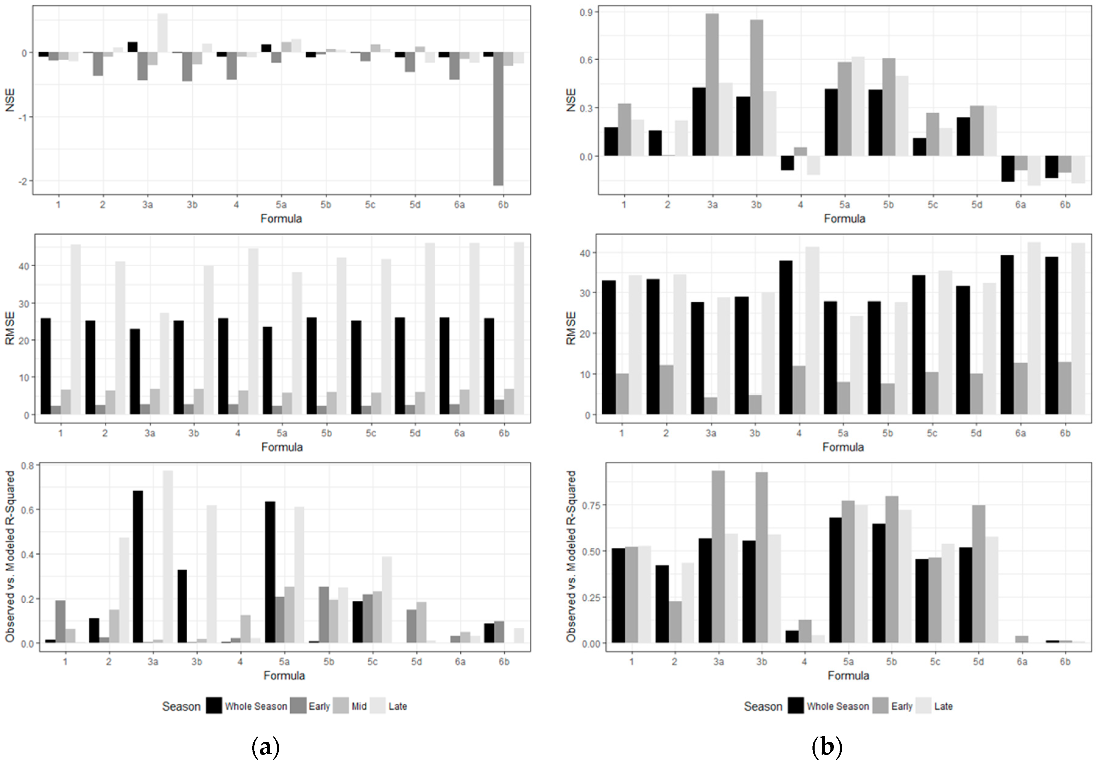
4.1. Single and Sub-Seasonal MLR Model Performance

Figure 3 shows the differences in performance of models based on forms from literature for the reservoirs and for the lake.

There was variable performance between sub-seasonal and single-season models using standard forms from literature for both Utah Lake and the reservoirs. Comparison of NSE for the reservoirs indicates exceptionally poor performance for all of the model forms. In contrast, for Utah Lake, some model forms (namely, 3a,b and 5a,b) have relatively high NSE, especially in the Early-season. With respect to RMSE, the single season generally results in intermediate model errors, (Late-season models are often greater for most standard forms compared to the single season), but the Early-season and Mid-season models have substantially lower errors. This is particularly interesting, because many of the models in literature been developed with a focus on the latter portion of the growing season. Values of RMSE for the Late-season reservoir models are close to those for Utah Lake model, despite the Utah Lake chl-a concentrations being substantially greater than those in the reservoirs, indicating that the models from literature were especially poor for the reservoirs in this study area. Finally, for the observed vs. modeled R², the sub-seasonal models generally perform better than the single-season models, though again, the Utah Lake models higher fit overall than the reservoir models.

Comparing the performance between algorithms that were specifically recommended for waters with high chl-a concentrations (most of those selected in this study) and those recommended for low chl-a concentrations (3a,b), there were relatively small differences in either the reservoirs (which do have relatively lower chl-a concentrations) or Utah Lake (which has consistently higher chl-a concentrations). For Utah Lake where there is concern over influence from suspended sediments and other constituents, we were especially interested in how models which have been used for similar cases in literature (4 and 5a–d) performed. Models 5a–d performed about the same as other models, and model 4 showed very poor skill (very low NSE and low R²).

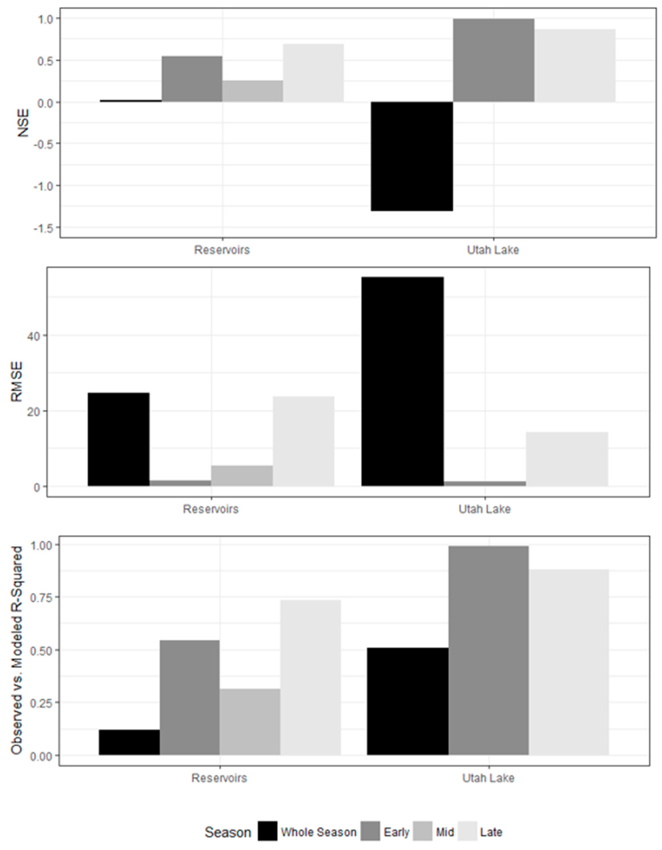
4.2. Sub-Seasonal MLSR Models and Model Performance

The resulting models from the single and sub-seasonal stepwise analysis differed greatly in selected predictor variables and in model performance. Comparisons of model performance are shown in Figure 4.

For both the reservoirs and Utah Lake, there is substantial improvement in NSE from single season to sub-seasonal models. Likewise, for each of the sub-seasonal models, there are lower model errors (RMSE) and better fit between observed and modeled values compared to the single season models. There is some variability between seasons; the Mid-season reservoir MLSR model still has a relatively low NSE and R² between observed and modeled values. This may be due to the loss in precision due to increasing the use of near-coincident data to ±24 h for this sub-season and rough approximations of the seasonal succession patterns.

The selected bands and measures of goodness of fit for the single season and sub-seasonal chl-a models are detailed in

Table 3. Summary of model parameterization and goodness of fit.

	Season	Selected Bands	NSE	RMSE	R2
Reservoirs	Whole Season	$\ln \left(B5\right), \frac{B3}{B4}, \frac{B3}{B7}, \ln \left(B3\right)$	0.02	24.7	0.12
	Early	$\frac{B2}{B3}, \frac{B4}{B3}$	0.54	1.5	0.54
	Mid	$\left(B4-B5\right), B2, \frac{B4}{B3}$	0.25	5.4	0.32
	Late	$B1,\ln \left(B1\right), \frac{B4}{B3}$	0.69	23.7	0.73
Utah Lake	Whole Season	$\frac{B4}{B1}, \ln \left(B1\right)$	−1.3	55.2	0.5
	Early	$\frac{B2}{B1}, B1, B5$	0.99	1.2	0.99
	Late	$B1, \frac{B2}{B7}, \frac{B3}{B7}$	0.86	14.4	0.88

(where B1 is Landsat Band 1, B2 is Landsat Band 2, etc.). The resulting models (with coefficients) are presented in Appendix A.

The step-wise method selected different predictor variables for the three models. However, there were some common terms across the sub-seasons that correlate to some of the suggested model forms from literature. The ratio of NIR and Red (B4/B3) is present in each of the sub-seasonal reservoir models (and B3/B4 was selected for the whole-season model). Based on the selected studies from literature, these bands were recommended for areas with higher chl-a concentrations. In contrast, this band ratio was not selected in either of the Utah Lake models, however Blue (B1) was selected for the sub-seasonal and whole-season models. In models from literature, B1 was used for lakes that were shallow and dominated by suspended sediment. Therein addition to these bands that are common among the sub-seasons, there are a wide variety of other bands, band combinations, and transforms that were also selected. This suggests that there may be a variety of influences, other in-lake constituents, or lake characteristics that contribute to the spectral signature of the water surface.

To demonstrate the skill of the models specific to their sub-season, we used the late-season models to estimate the chl-a for other sub-seasons. This would be comparable to commonly reported approaches where models developed with a single satellite image are applied to other images at other times in the growing season.

Table 4. Comparison of sub-seasonal model skill (observed vs. modeled R²) to single (late) model applied to early and mid-season data and aggregate model.

Model Application	R2	R2 with Season-Specific Model
Reservoir Late-model to Early-data	0.4	0.48
Reservoir Late-model to Mid-data	0.08	0.32
Lake Late-model to Early-data	0.95	0.98

shows that in both cases of the lake and reservoirs, the skill of the late-season model is lower when used to estimate data in these other seasons, with slight decrease in correlation for both the Early-seasons for the reservoirs and the lake, and a substantial decrease in skill for the Mid-season reservoir model.

We attribute this difference in skill to the fact that the sub-seasonal models account for the different physical and spectral characteristics of dominant algal populations specific to each growing season and thus provide more accurate estimations throughout the growing season than a single model. This is true whether the single model was an aggregate of all data, or when a model for one time period is applied to another time period. As expected, the model developed using all the data performed better than ones developed with data from one season then applied to a different season. Clearly, the season-specific models showed the most skill.

5. Discussion

This study demonstrates the importance of considering specific optical, physical, and biological characteristics when developing empirical remote sensing models. The poor performance of algorithms used in literature for the lake and reservoirs in this case study suggests that a one-size-fits-all approach to variable selection and model development may result in poor predictive ability. While these models may have performed well in the original study areas, the MLR calibration approach shows that these relationships do not directly transfer to either the case of the reservoirs (relatively deep, clear water with low to medium chl-a concentrations) or Utah Lake (shallow, highly turbid lake, with moderate to extreme chl-a concentrations). The data-driven technique for model parameterization resulted in selection of several common bands from literature that were somewhat reflective of the unique characteristics of the lake and reservoirs. This supports the findings and recommendations of these previous studies, which have used the Red/NIR relationships and the Blue band of Landsat to estimate chl-a in high chl-a conditions and shallow lakes, respectively. The selection of other bands, however, indicates that there are other important factors that are influencing the remotely sensed signature. These factors may include unique populations of algae, color from suspended sediments or mineral precipitates, reflectance from the bottom of the shallow lake. This means that when applying the models to water bodies with differing optical characteristics, it is especially important to consider the influence other these other constituents and factors, rather than assuming a direct application of relationships found in literature for other water bodies. While the focus of this study was on model parameterization, it would be important an independent validation of the models would help determine suitability for long-term applications.

6. Conclusions

We demonstrated the use of a simple data driven, statistical learning technique to create season-specific remote sensing models that account for some of these external influences to surface reflectance. In general, these models which account for other optical characteristics more accurately estimate water quality conditions, during the entire growing season. In addition to consideration of bands outside of those cited in literature, this method generally allows for more complex correlations to be considered in the models through the use of band ratios or other transforms. Other more computationally challenging data-driven techniques, such as artificial neural networks or decision trees may capture the complexity and additional effects better than a linear modeling approach, though these models may also be informed by including information about seasonal succession patterns and population dynamics.

We feel the approach of sub-seasonal models, especially those that consider a broader potential number of predictor variables offers a vast improvement over single-season models that are limited to forms used in other regions. This improvement makes the models more robust and suitable for use with historical Landsat images throughout the entire growing season. A move towards greater accuracy during the entire growing season will improve understanding of long-term trends and patterns (i.e., determining whether high chl-a concentrations and the onset of blooms are shifting earlier in the growing season).

Chl-a estimates obtained from Landsat images can help overcome issues of missing or incomplete historical data, providing “something” for “nothing” as the models can provide estimates for dates with missing field-sampling data at minimal cost. These Landsat estimates can then be validated (and models updated) with ongoing field sampling campaigns (ideally targeting dates with satellite overpass for optimal model development). This will make monitoring and modeling more efficient. In addition, while out-of-sample applications may not be as accurate as in-sample applications, a robust set of models that is well-suited for describing changes in conditions throughout the growing season will provide valuable information on trends and context (e.g., historic maxima, minima, and variation).

Future work and extensions include applying these techniques to additional locations and use of other remote sensing data. These methods could also be applied to other parameters that can be estimated using remotely sensed data such as turbidity, Secchi depth, or phycocyanin concentrations.

References

1. Hambrook Berkman, J.A.; Canova, M.G. Algal biomass indicators. In U.S.G.S. Techniques of Water-Resources Investigations, Volume 9; United States Geological Survey: Reston, VA, USA, 2007; Section 7.4. [Google Scholar]
2. Stadelmann, T.H.; Brezonik, P.L.; Kloiber, S. Seasonal patterns of chlorophyll a and Secchi disk transparency in lakes of east-central Minnesota: Implications for design of ground-and satellite-based monitoring programs. Lake Reserv. Manag. 2001, 17, 299–314. [Google Scholar] [CrossRef]
3. Hansen, C.; Swain, N.; Munson, K.; Adjei, Z.; Williams, G.P.; Miller, W. Development of sub-seasonal remote sensing chlorophyll-a detection models. Am. J. Plant Sci. 2013, 4, 21. [Google Scholar] [CrossRef]
4. Hansen, C.H.; Williams, G.P.; Adjei, Z. Long-term application of remote sensing chlorophyll detection models: Jordanelle reservoir case study. Nat. Resour. 2015, 6, 123. [Google Scholar] [CrossRef]
5. Hansen, C.H.; Williams, G.P.; Adjei, Z.; Barlow, A.; Nelson, E.J.; Miller, A.W. Reservoir water quality monitoring using remote sensing with seasonal models: Case study of five central-Utah reservoirs. Lake Reserv. Manag. 2015, 31, 225–240. [Google Scholar] [CrossRef]
6. Giardino, C.; Brando, V.E.; Dekker, A.G.; Strömbeck, N.; Candiani, G. Assessment of water quality in lake garda (Italy) using Hyperion. Remote Sens. Environ. 2007, 109, 183–195. [Google Scholar] [CrossRef]
7. Giardino, C.; Pepe, M.; Brivio, P.A.; Ghezzi, P.; Zilioli, E. Detecting chlorophyll, Secchi disk depth and surface temperature in a sub-alpine lake using Landsat imagery. Sci. Total Environ. 2001, 268, 19–29. [Google Scholar] [CrossRef]
8. Yacobi, Y.Z.; Gitelson, A.; Mayo, M. Remote sensing of chlorophyll in lake Kinneret using Highspectral-resolution radiometer and Landsat TM: Spectral features of reflectance and algorithm development. J. Plankton Res. 1995, 17, 2155–2173. [Google Scholar] [CrossRef]
9. Chander, G.; Markham, B.L.; Helder, D.L. Summary of current radiometric calibration coefficients for Landsat MSS, TM, ETM+, and EO-1 Ali sensors. Remote Sens. Environ. 2009, 113, 893–903. [Google Scholar] [CrossRef]
10. Duan, H.; Ma, R.; Xu, X.; Kong, F.; Zhang, S.; Kong, W.; Hao, J.; Shang, L. Two-decade reconstruction of algal blooms in china’s lake Taihu. Environ. Sci. Technol. 2009, 43, 3522–3528. [Google Scholar] [CrossRef] [PubMed]
11. Ho, J.C.; Stumpf, R.P.; Bridgeman, T.B.; Michalak, A.M. Using Landsat to extend the historical record of lacustrine phytoplankton blooms: A Lake Erie case study. Remote Sens. Environ. 2017, 191, 273–285. [Google Scholar] [CrossRef]
12. Olmanson, L.G.; Bauer, M.E.; Brezonik, P.L. A 20-year Landsat water clarity census of Minnesota’s 10,000 lakes. Remote Sens. Environ. 2008, 112, 4086–4097. [Google Scholar] [CrossRef]
13. Matthews, M.W. A current review of empirical procedures of remote sensing in inland and near-coastal transitional waters. Int. J. Remote Sens. 2011, 32, 6855–6899. [Google Scholar] [CrossRef]
14. Hansen, C.H.; Burian, S.J.; Dennison, P.E.; Williams, G.P. Spatiotemporal variability of lake water quality in the context of remote sensing models. Remote Sens. 2017, 9, 409. [Google Scholar] [CrossRef]
15. Kloiber, S.M.; Brezonik, P.L.; Olmanson, L.G.; Bauer, M.E. A procedure for regional lake water clarity assessment using Landsat multispectral data. Remote Sens. Environ. 2002, 82, 38–47. [Google Scholar] [CrossRef] [Green Version]
16. Nelson, S.A.; Soranno, P.A.; Cheruvelil, K.S.; Batzli, S.A.; Skole, D.L. Regional assessment of lake water clarity using satellite remote sensing. J. Limnol. 2003, 62, 27–32. [Google Scholar] [CrossRef]
17. Lesht, B.M.; Barbiero, R.P.; Warren, G.J. A band-ratio algorithm for retrieving open-lake chlorophyll values from satellite observations of the great lakes. J. Great Lakes Res. 2013, 39, 138–152. [Google Scholar] [CrossRef]
18. Woźniak, M.; Bradtke, K.M.; Darecki, M.; Krężel, A. Empirical model for phycocyanin concentration estimation as an indicator of cyanobacterial bloom in the optically complex coastal waters of the Baltic sea. Remote Sens. 2016, 8, 212. [Google Scholar] [CrossRef]
19. Gordon, H.R.; Morel, A.Y. Remote Assessment of Ocean Color for Interpretation of Satellite Visible Imagery: A Review; Springer Science & Business Media: New York, NY, USA, 2012; Volume 4. [Google Scholar]
20. Morel, A.; Prieur, L. Analysis of variations in ocean color 1. Limnol. Oceanogr. 1977, 22, 709–722. [Google Scholar] [CrossRef]
21. O’Reilly, J.E.; Maritorena, S.; Mitchell, B.G.; Siegel, D.A.; Carder, K.L.; Garver, S.A.; Kahru, M.; McClain, C. Ocean color chlorophyll algorithms for Seawifs. J. Geophys. Res. Oceans 1998, 103, 24937–24953. [Google Scholar] [CrossRef]
22. Mobley, C.D.; Sundman, L.K.; Davis, C.O.; Bowles, J.H.; Downes, T.V.; Leathers, R.A.; Montes, M.J.; Bissett, W.P.; Kohler, D.D.; Reid, R.P. Interpretation of hyperspectral remote-sensing imagery by spectrum matching and look-up tables. Appl. Opt. 2005, 44, 3576–3592. [Google Scholar] [CrossRef] [PubMed]
23. Mobley, C.D. Estimation of the remote-sensing reflectance from above-surface measurements. Appl. Opt. 1999, 38, 7442–7455. [Google Scholar] [CrossRef] [PubMed]
24. Toole, D.A.; Siegel, D.A.; Menzies, D.W.; Neumann, M.J.; Smith, R.C. Remote-sensing reflectance determinations in the coastal ocean environment: Impact of instrumental characteristics and environmental variability. Appl. Opt. 2000, 39, 456–469. [Google Scholar] [CrossRef] [PubMed]
25. Han, L. Spectral reflectance with varying suspended sediment concentrations in clear and algae-laden waters. Photogram. Eng. Remote Sens. 1997, 63, 701–705. [Google Scholar]
26. Mittenzwey, K.H.; Ullrich, S.; Gitelson, A.; Kondratiev, K. Determination of chlorophyll a of inland waters on the basis of spectral reflectance. Limnol. Oceanogr. 1992, 37, 147–149. [Google Scholar] [CrossRef] [Green Version]
27. Tan, J.; Cherkauer, K.A.; Chaubey, I.; Troy, C.D.; Essig, R. Water quality estimation of river plumes in southern lake Michigan using Hyperion. J. Great Lakes Res. 2016, 42, 524–535. [Google Scholar] [CrossRef]
28. Olmanson, L.G.; Brezonik, P.L.; Bauer, M.E. Airborne hyperspectral remote sensing to assess spatial distribution of water quality characteristics in large rivers: The Mississippi river and its tributaries in Minnesota. Remote Sens. Environ. 2013, 130, 254–265. [Google Scholar] [CrossRef]
29. Tan, J.; Cherkauer, K.A.; Chaubey, I. Using hyperspectral data to quantify water-quality parameters in the Wabash river and its tributaries, Indiana. Int. J. Remote Sens. 2015, 36, 5466–5484. [Google Scholar] [CrossRef]
30. Bartholomew, P.J. Mapping and Modeling Chlorophyll-a Concentrations in the Lake Manassas Reservoir Using Landsat Thematic Mapper Satellite Imagery. Master’s Thesis, Virginia Tech, Blacksburg, VA, USA, 2003. [Google Scholar]
31. Boyer, J.N.; Kelble, C.R.; Ortner, P.B.; Rudnick, D.T. Phytoplankton bloom status: Chlorophyll a biomass as an indicator of water quality condition in the southern Estuaries of Florida, USA. Ecol. Indic. 2009, 9, S56–S67. [Google Scholar] [CrossRef]
32. Östlund, C.; Flink, P.; Strömbeck, N.; Pierson, D.; Lindell, T. Mapping of the water quality of lake Erken, Sweden, from imaging spectrometry and Landsat thematic mapper. Sci. Total Environ. 2001, 268, 139–154. [Google Scholar] [CrossRef]
33. Brezonik, P.; Menken, K.D.; Bauer, M. Landsat-based remote sensing of lake water quality characteristics, including chlorophyll and colored dissolved organic matter (CDOM). Lake Reserv. Manag. 2005, 21, 373–382. [Google Scholar] [CrossRef]
34. Fuller, L.M.; Aichele, S.S.; Minnerick, R.J. Predicting Water Quality by Relating Secchi-Disk Transparency and Chlorophyll a Measurements to Satellite Imagery for Michigan Inland Lakes, August 2002; US Department of the Interior, US Geological Survey: Reston, VA, USA, 2004.
35. Lin, S.; Novitski, L.N.; Qi, J.; Stevenson, R.J. Landsat TM/ETM+ and machine-learning algorithms for limnological studies and algal bloom management of inland lakes. J. Appl. Remote Sens. 2018, 12, 026003. [Google Scholar] [CrossRef]
36. Brooks, B.W.; Lazorchak, J.M.; Howard, M.D.; Johnson, M.V.V.; Morton, S.L.; Perkins, D.A.; Reavie, E.D.; Scott, G.I.; Smith, S.A.; Steevens, J.A. In some places, in some cases, and at some times, harmful algal blooms are the greatest threat to inland water quality. Environ. Toxicol. Chem. 2017, 36, 1125–1127. [Google Scholar] [CrossRef] [PubMed] [Green Version]
37. Utah Department of Environmental Quality (UDEQ). Jordanelle Reservoir Lake Report; UDEQ: Salt Lake City, UT, USA, 2004.
38. Utah Department of Environmental Quality (UDEQ). Deer Creek Reservoir Lake Report; UDEQ: Salt Lake City, UT, USA, 2004.
39. Utah Department of Environmental Quality (UDEQ). Utah Lake Report; UDEQ: Salt Lake City, UT, USA, 2006.
40. Oberndorfer, R.; Central Utah Water Conservancy District, Salt Lake City, UT, USA; Hansen, C.H.; University of Utah, Salt Lake City, UT, USA. Reservoir condition discussion and suggested seasons. Personal communication, 2014. [Google Scholar]
41. Whiting, M.C.; Brotherson, J.D.; Rushforth, S.R. Environmental interaction in summer algal communities of Utah Lake. Great Basin Nat. 1978, 38, 31–41. [Google Scholar]
42. Rushforth, S.R.; Squires, L.E. New records and comprehensive list of the algal taxa of Utah lake, Utah, USA. Great Basin Nat. 1985, 45, 237–254. [Google Scholar]
43. Gorelick, N.; Hancher, M.; Dixon, M.; Ilyushchenko, S.; Thau, D.; Moore, R. Google earth engine: Planetary-scale geospatial analysis for everyone. Remote Sens. Environ. 2017, 202, 18–27. [Google Scholar] [CrossRef]
44. Masek, J.G.; Vermote, E.F.; Saleous, N.E.; Wolfe, R.; Hall, F.G.; Huemmrich, K.F.; Gao, F.; Kutler, J.; Lim, T.-K. A Landsat surface reflectance dataset for North America, 1990–2000. Geosci. Remote Sens. Lett. IEEE 2006, 3, 68–72. [Google Scholar] [CrossRef]
45. Johnson, R.; Strutton, P.G.; Wright, S.W.; McMinn, A.; Meiners, K.M. Three improved satellite chlorophyll algorithms for the Southern Ocean. J. Geophys. Res. Oceans 2013, 118, 3694–3703. [Google Scholar] [CrossRef] [Green Version]
46. Draper, N.R.; Smith, H. Applied Regression Analysis; John Wiley & Sons: New York, NY, USA, 2014; Volume 326. [Google Scholar]
47. Montgomery, D.C.; Peck, E.A.; Vining, G.G. Introduction to Linear Regression Analysis; John Wiley & Sons: New York, NY, USA, 2012. [Google Scholar]
48. Sass, G.Z.; Creed, I.F.; Bayley, S.E.; Devito, K.J. Understanding variation in trophic status of lakes on the boreal plain: A 20 years retrospective using Landsat tm imagery. Remote Sens. Environ. 2007, 109, 127–141. [Google Scholar] [CrossRef]
49. Lathrop, R.G., Jr. Landsat thematic mapper monitoring of turbid inland water quality. Photogram. Eng. Remote Sens. 1992, 465–470. [Google Scholar]
50. Duan, H.; Zhang, Y.; Zhang, B.; Song, K.; Wang, Z. Assessment of chlorophyll-a concentration and trophic state for lake Chagan using Landsat tm and field spectral data. Environ. Monit. Assess. 2007, 129, 295–308. [Google Scholar] [CrossRef] [PubMed]
51. Gitelson, A.; Garbuzov, G.; Szilagyi, F.; Mittenzwey, K.H.; Karnieli, A.; Kaiser, A. Quantitative remote sensing methods for real-time monitoring of inland waters quality. Int. J. Remote Sens. 1993, 14, 1269–1295. [Google Scholar] [CrossRef]
52. Mayo, M.; Gitelson, A.; Yacobi, Y.; Ben-Avraham, Z. Chlorophyll distribution in lake Kinneret determined from Landsat thematic mapper data. Remote Sens. 1995, 16, 175–182. [Google Scholar] [CrossRef]
53. Brivio, P.; Giardino, C.; Zilioli, E. Determination of chlorophyll concentration changes in lake garda using an image-based radiative transfer code for Landsat tm images. Int. J. Remote Sens. 2001, 22, 487–502. [Google Scholar] [CrossRef]
54. Tyler, A.; Svab, E.; Preston, T.; Présing, M.; Kovács, W. Remote sensing of the water quality of shallow lakes: A mixture modelling approach to quantifying phytoplankton in water characterized by high-suspended sediment. Int. J. Remote Sens. 2006, 27, 1521–1537. [Google Scholar] [CrossRef]
55. Sudheer, K.; Chaubey, I.; Garg, V. Lake water quality assessment from Landsat thematic mapper data using neural network: An approach to optimal band combination selection1. J. Am. Water Resour. Assoc. 2006, 42, 1683–1695. [Google Scholar] [CrossRef]
56. Wang, F.; Han, L.; Kung, H.T.; Van Arsdale, R.B. Applications of Landsat-5 TM imagery in assessing and mapping water quality in Reelfoot lake, Tennessee. Int. J. Remote Sens. 2006, 27, 5269–5283. [Google Scholar] [CrossRef]
57. Lathrop, R.G.; Lillesand, T.M. Use of thematic mapper data to assess water quality in green bay and central lake Michigan. Photogram. Eng. Remote Sens. 1986, 52, 671–680. [Google Scholar]
58. Mouw, C.B.; Greb, S.; Aurin, D.; DiGiacomo, P.M.; Lee, Z.; Twardowski, M.; Binding, C.; Hu, C.; Ma, R.; Moore, T. Aquatic color radiometry remote sensing of coastal and inland waters: Challenges and recommendations for future satellite missions. Remote Sens. Environ. 2015, 160, 15–30. [Google Scholar] [CrossRef]
59. Wang, M.; Shi, W. The NIR-SWIR combined atmospheric correction approach for Modis ocean color data processing. Opt. Express 2007, 15, 15722–15733. [Google Scholar] [CrossRef] [PubMed]
60. Gordon, H.R. Removal of atmospheric effects from satellite imagery of the oceans. Appl. Opt. 1978, 17, 1631. [Google Scholar] [CrossRef] [PubMed]
61. Nash, J.E.; Sutcliffe, J.V. River flow forecasting through conceptual models part I—A discussion of principles. J. Hydrol. 1970, 10, 282–290. [Google Scholar] [CrossRef]
62. Casterlin, M.E.; Reynolds, W.W. Seasonal algal succession and cultural eutrophication in a north temperate lake. Hydrobiologia 1977, 54, 99–108. [Google Scholar] [CrossRef]
63. Kutser, T. Quantitative detection of chlorophyll in cyanobacterial blooms by satellite remote sensing. Limnol. Oceanogr. 2004, 49, 2179–2189. [Google Scholar] [CrossRef] [Green Version]
Figure 1. Study area in north-central Utah including the Jordanelle Reservoir, Deer Creek Reservoir, and Utah Lake which are linked via the Provo River.
Hydrology 05 00062 g001
Figure 2. Surface Reflectance Values by Landsat Band (Blue, Green, Red, Near Infrared (NIR) and Shortwave Infrared (SWIR1 and SWIR2)) for the (a) reservoirs (Deer Creek and Jordanelle) and (b) Utah Lake.
Hydrology 05 00062 g002
Figure 3. Comparison of Model Performance for single and sub-seasonal (a) reservoir models and (b) Utah Lake models created using multiple linear regression (MLR) and standard forms from literature.
Hydrology 05 00062 g003
Figure 4. Comparison of Model Performance between single and sub-seasonal models created using Multiple Linear Stepwise Regression (MLSR).
Hydrology 05 00062 g004