Abstract
Nowadays, increased flood risk is recognized as one of the most significant threats in most parts of the world, with recurring severe flooding events causing significant property and human life losses. This has entailed public debates on both the apparent increased frequency of extreme events and the perceived increases in rainfall intensities within climate changing scenarios. In this work, a stationary vs. Non-Stationary Analysis of annual extreme rainfall was performed with reference to the case studies of the African cities of Dar Es Salaam (TZ) and Addis Ababa (ET). For Dar Es Salaam (TZ) a dataset of 53 years (1958–2010) of maximum daily rainfall records (24 h) was analysed, whereas a 47-year time series (1964–2010) was taken into account for Addis Ababa (ET). Both gauge stations rainfall data were suitably fitted by Extreme Value Distribution (EVD) models. Inference models using the Maximum Likelihood Estimation (MLE) and the Bayesian approach were applied on EVD considering their impact on the shape parameter and the confidence interval width. A comparison between a Non-Stationary regression and a Stationary model was also performed. On this matter, the two time series did not show any Non-Stationary effect. The results achieved under the CLUVA (Climatic Change and Urban Vulnerability in Africa) EU project by the Euro-Mediterranean Centre for Climate Change (CMCC) (with 1 km downscaling) for the IPCC RCP8.5 climatological scenario were also applied to forecast the analysis until 2050 (93 years for Dar Es Salaam TZ and 86 years for Addis Ababa ET). Over the long term, the process seemed to be Non-Stationary for both series. Moreover, with reference to a 100-year return period, the IDF (Intensity-Duration-Frequency) curves of the two case-studies were estimated by applying the Maximum Likelihood Estimation (MLE) approach, as a function of confidence intervals of 2.5% and 97.5% quantiles. The results showed the dependence of Non-Stationary effects of climate change to be conveniently accounted for engineering design and management.
1. Introduction
Nowadays, the increased flood risk is recognized as one of the most important threats, from both the actual and, more importantly, the climate change scenario, with frequent severe flooding at the global scale causing significant loss of property and life. In 2009 (Messina, Sicily Region), 2010 (Atrani, Campania Region) and 2011 (Genova, Liguria Region), the Italian territory was forced to face widespread flooding events, highlighting the significant vulnerability of the territory and the inadequacy of early warning and flood protection systems. According to the official report of the Italian Environmental Ministry, over 1000 buildings and businesses were flooded, causing 40 deaths. Nevertheless, worldwide flooding events caused by extreme rainfall events are causing the degradation of water quality, damages and potential loss of life [1,2].
These events prompted public debates on the apparent causes of the increased frequency of extreme events. Indeed, scientists are querying the changing statistics of rainfall intensity, especially considering the climate model predictions of increasing frequency and intensity of heavy rainfall in the high latitudes under enhanced greenhouse conditions. In 2007, the United Nations Intergovernmental Panel on Climate Change (IPCC) issued a report [3] stating that “It is very likely that hot extremes, heat waves, and heavy precipitation events will continue to become more frequent”, with the “very likely” assertion indicating an occurrence probability greater than 90%. Thus, the actual and recent observations and future predictions are pointing out the importance of suitable assessments of the probability occurrence of extreme events related to long return periods T.
A comprehensive review of trend analysis and climate change projections of extreme precipitations in Europe is given by [4]. Many studies demonstrate changes in seasonal extreme precipitations in some parts of Europe [5,6,7,8].
To estimate extreme value statistics for frequency analysis of extreme precipitation, the assumption of stationarity is valid if we do not consider changes in climate that affect the hydrological regime. In this matter, during the last decade, several studies adopted Non-Stationary frequency analysis for extreme precipitation in different parts of the world [9,10,11]. On the other hand, simplified indexes [12,13] or Innovative Trend Analysis [14] have also been applied and tested for identifying potential trends in extreme precipitations.
Extreme Value Distributions (EVDs) are usually able to accurately represent the frequency of hydrologic over-threshold physical processes. Parameter estimation through Likelihood-based methods allows extreme quantiles to be calculated, providing the appraisal of the parameter and the associated dynamic for given return period T (e.g., 100 years). However, EVD parameters are typically estimated from the extremes of a dataset (e.g., annual maxima), which may result in characterizing unrealistic values. A possible solution to improve the reliability of statistical analysis concerns the application of a Bayesian framework, which allows us to constrain the estimates as a function of predefined information, which could realistically reproduce the hydrologic processes governing the available data. Further essential points regard the potential Non-Stationarity that could involve meaningful variation of the mean value of the distribution, with corresponding variation of the return levels related to a return period T.
This work first investigated the behaviour of the GEV distribution to estimate the annual maxima of rainfall depths adopting both MLE and Bayesian methods, evaluating their relative impacts on the confidence interval widths. Moreover, stationary and Non-Stationary analyses of extreme rainfall were applied to historical time series (with a relative limited extension), and the extended ones used climate models, thus evaluating potential Non-Stationary effects induced by the climate models.
Maximum daily (24 h) rainfall data series for the cities of Dar Es Salaam (TZ) with a 53-year dataset (1958–2010), and Addis Ababa (ET) with a 47-year dataset (1964–2010) were analysed to evaluate the Goodness of Fit (GoF) of EVD models. Specifically, a comparison was realized between Maximum Likelihood Estimation (MLE) and Bayesian models. Moreover, results gathered from the CLUVA (Climatic Change and Urban Vulnerability in Africa) EU project by the Euro-Mediterranean Centre for Climate Change (CMCC) (with 1 km downscaled resolution) for the IPCC RCP8.5 climatological scenario were also considered, extending the rainfall dataset to 2050 (93 years for Dar Es Salaam TZ and 87 years for Addis Ababa ET).
The impact of the actual versus changing hydrologic forcing scenarios was evaluated, with reference to a 100-year return period, estimating the Intensity-Duration-Frequency (IDF) curves through the Maximum Likelihood Estimation (MLE) as a function of confidence intervals of 16% and 84% quantiles, respectively.
2. Methodology
2.1. Extreme Value Theory
The Generalized Extreme Value (GEV) distribution was proposed by [15] following the original formulation of [16]. The GEV approach is widely applied to model extremes of hydrologic processes such as floods [17], rainfall [18] and sea waves [19]. Further applications also include different subjects such as financial market risk modelling [20].
By supposing X1, X2, …, Xn as a sequence of independent random variables from a common distribution function F, the statistic order of interest is Mn = max{X1, X2, …, Xn}, namely, the maximal value of the independent identically distributed (i.i.d.) random variables. Here, Xi represents the daily rainfall amount (mm) and n the number of observations in one year (365 or 366), so that Mn is the annual maximum. When the parent distribution function F is known, the distribution of Mn can be derived from statistical theory such that P(Mn ≤ z) = [F(z)]n.
With F unknown, a limit distribution for Fn as n → ∞ is searched for, in a way similar to how the application of the Central Limit Theorem (CLT) allows approximation of the distribution of samples by means of the Normal distribution. Considering the linearly renormalized variable M*n:
for sequences an > 0 and bn, Mn should be normalized because Fn(z) → 0 as n → ∞ for fixed z lower than the upper end-point of F. This causes the degeneration of the distribution to a point mass on the upper end-point of F (i.e., the smallest z such that F(z) = 1).
The whole range of limit distributions for M*n is given by the Extremal Types Theorem [21]. If a series of constants {an > 0} and {bn} exists, such that P(M*n ≤ z) → G(z) as n → ∞ (with G a non-degenerate distribution function), then G must be included into one of the following three families: (I) Gumbel; (II) Fréchet and (III) Weibull distributions.
Families I, II and III can be combined into a single family named the Generalized Extreme Value (GEV) distribution [4], given by the following Equation (2):
defined as {z: 1 + ξ(z − μ)/σ > 0}, where μ, σ, ξ are the location, scale and shape parameters, respectively.
The shape parameter ξ governs the tail behaviour of the distribution at its upper end. The Weibull class has a finite upper endpoint, whereas the Gumbel and Fréchet classes provide relatively different rates of decay in the tail. The Fréchet is a more heavy tailed distribution because it decays polynomially with respect to the Gumbel class, which decays exponentially instead. The tail behaviour is strongly significant, as it corresponds to quite different characteristics of extreme value behaviour. To perform the unification to a single GEV distribution, making a choice about the best model before parameter estimation is required. The key advantage of the GEV distribution over the three EV types derives from the assertion that the estimation of the ξ parameter via inference methods allows the data to select which family (and tail behaviour) to adopt without any prior decision. Moreover, the uncertainty in the estimated value of ξ measures the uncertainty correlated with the effectiveness of the three types for the available data set.
By inverting Equation (2), an estimation of extreme quantiles can be obtained, being the pth-upper quantile of the z distribution given by G(zp) = 1 − p. A zp estimation is achieved by substituting the estimates of μ, σ and ξ (for 0 < p < 1):
where zp is the return level correlated to the return period T = 1/p. Return levels represent usual estimation parameters for extreme events, resulting in the “100-year flood” widely applied in hydrological applications for civil engineering. Loosely speaking, zp is the level expected to be meanly exceeded once every 1/p years (assuming G as the annual maximum). More formally, for extreme rainfall, zp is the daily rainfall amount exceeded by the annual maximum for any year with a probability equal to p.
The plot of zp against 1/p is known as the return level plot, resulting in an effective tool to graphically observe the return levels. The sign of the shape parameter takes on an important role when extrapolating to long return periods. Indeed, a small error in estimating the ξ parameter can lead to a much larger error in the return level estimation. Thus, accurate evaluation of the GEV shape parameter is essential to plan and develop flood protection models [22].
2.2. Bayesian Approach
The Bayesian approach allows us to make inferences from the Likelihood function, overcoming the limitation of the usually small size of the time series characterized by the annual maxima.
According to this approach, as opposed to the MLE, a parameter θ of a distribution is not an unknown constant but it is treated as a random variable related to a prior normal pdf with zero mean and a certain variance .
If we consider as independent realizations of a random variable so that , according to the Bayes Theorem:
where is the posterior distribution, is the abovementioned prior distribution and is the Likelihood. In case of many parameters such as the GEV distribution, the denominator of Equation (4) can be computationally complex. To overcome this issue, Markov Chain Monte Carlo (MCMC) techniques, based on multiple simulations, are usually adopted [21].
The sequences of simulated values of the parameters can be generated with the Metropolis-Hastings algorithm, e.g., applying the evdbayes package within R software [23]. The algorithm generates a sequence of parameters adopting a random-walk characterized by a normal distribution with a mean equal to the previous value of the parameter in the chain and a given variance. After a burn-in period, the sequence of the parameters is approximately stationary and the estimate of the parameter is computed as the mean of the sequence excluding the values within the burn-in period.
2.3. Non-Stationary Frequency Model
Under the climate change context, the intensity and/or the frequency of extreme rainfall events can change with time, so that the hypothesis of stationarity of the series of annual maxima is not satisfied [24].
The Non-Stationary behavior of an extreme value distribution can be expressed in different ways, such as changing its average values, the variability of its variables or both of them simultaneously [25]. More complex cases of Non-Stationarity could involve changes in distribution asymmetry or even in the parametric form [24].
Most studies look at trends induced by average variables [26] or extreme values indicators [27] without considering the variation of the shape of the distribution or of its variability. Following this simplest hypothesis, in this work, the GEV distribution for a Non-Stationary frequency model is expressed as GEV(μi, σ, ξ), where μi = μ0 + μtrend ti, with ti the counter of the year from the analysed time series (see Section 3.1.1).
3. Case Studies
The extreme value statistics for frequency analysis of extreme precipitation were performed for Dar Es Salaam (TZ) and Addis Ababa (ET) case studies for both cases of historical data and extended time series using the COSMO CLM model by Euro-Mediterranean Centre for Climate Change (CMCC). Table 1 shows the basic statistics of the mentioned time series. Kolmogorov-Smirnov, Anderson-Darling and Chi-Square GoF tests have been performed on the GEV distribution application for both case studies related to the historical and extended time series. Results of the GoF were positive for each test, considering the rejection of the null hypothesis at the level a = 0.01.

Table 1.
Basic statistics of the times series for both cases studies of Dar Es Salaam and Ababa.
3.1. Dar Es Salaam (TZ) Rainfall Data
3.1.1. Historical Data
The first analysis was based on the data series of daily rainfall observations recorded at Dar Es Salaam (TZ) Airport, Tanzania (Latitude: −6.87 N; Longitude: 39.20 E; Elevation: 53 m a.s.l.) with reference to the time span 1 January 1958–31 December 2010. Annual maxima are plotted in the following Figure 1.
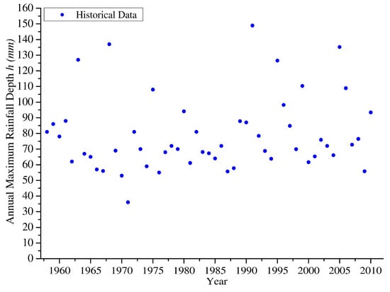
Figure 1.
Annual maximum 24 h rainfalls recorded at Dar Es Salaam TZ (1958–2010).
The assumption of data as independent observations from the GEV distribution was applied. Based on the Maximum Likelihood Estimation (MLE) method (by using the eXtremes [28] and evd [29] packages in R software [30]), the following estimation of μ, σ and ξ parameters was obtained (, , ) = (68.25, 16.93, 0.039), with standard errors equal to 2.55, 1.83 and 0.083, respectively. Approximate 95% confidence intervals for each parameter were [63.25, 73.25], [13.35, 20.52] and [−0.124, 0.202] for μ, σ and ξ, respectively. This showed that the 95% confidence interval is well extended for values lower than zero, although the estimation of the shape parameter was positive, pointing out the uncertainty of the performed evaluation.
The survey for the 100-year return level was = 153.6 mm, with a 95% confidence interval of [129, 208] mm, and the return level plot in Figure 2 shows the linear trend of the function as a consequence of the estimation of the ξ parameter tending towards 0. Diagnostic plots (not shown for the sake of brevity), such as probability plot and quantile plots, showed that each set of plotted points are roughly linear, validating the use of the GEV model.
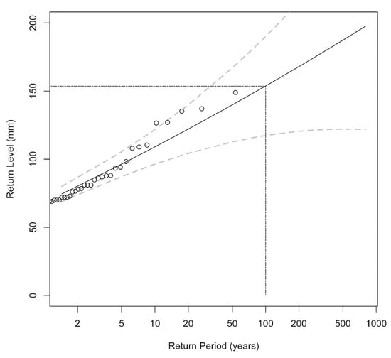
Figure 2.
Return Level (in mm) plot using maximum likelihood surveys.
A more reliable survey using a Bayesian approach was implemented by applying the evdbayes package in R software [23]. The algorithm provides functions for the Bayesian analysis of extreme value models, using the Markov Chain Monte Carlo (MCMC) method. The solely genuine prior information available referred to the GEV shape parameter; thus, prior information about μ and σ parameters were not-informative normal distributions with variance 104. In the Bayesian analysis, more specific empirical evidence provided by Koutsoyiannis [31,32] was applied, as a function of ξ ≈ 0.15 for Europe.
A normal distribution around 0.15 with variance 0.2 was formed, restricting the ξ variation to a physically reasonable range [22]. By applying the MLEs as the initial vector θ0 = (, , ) = (68.25, 16.93, 0.039) and the proposal standard deviations psd = (6.191, 0.230, 0.216) (identified with some pilot runs), a Markov Chain Monte Carlo (MCMC method) was generated with a length of 100,000, satisfying mixing properties (Figure 3). By graphically examining the chain (Figure 3) and using the Geweke diagnostic [33], a burn-in period of 10 iterations was found.
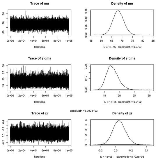
Figure 3.
MCMC realizations of the GEV parameters with a Bayesian analysis of the Dar Es Salaam (TZ) rainfall data.
The sample means and standard deviations of each marginal component of the chain were:
whereas the 95% reasonable intervals were [63.10, 73.52], [14.32, 22.12] and [−0.11, 0.22] for μ, σ, and ξ, respectively.
The sequence of simulated (μi, σi, ξi) values was transformed, leading to a sample from the corresponding posterior distribution of the 100-year return level (Figure 4). This gave a estimation equal to 161.8 mm with 95% reasonable interval of [131.6, 219.1] mm. The plot of the posterior return level given in Figure 5 shows the upper 95% interval to be more remote than the lower interval from the median level.
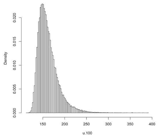
Figure 4.
Estimated posterior density of the 100-year return level.
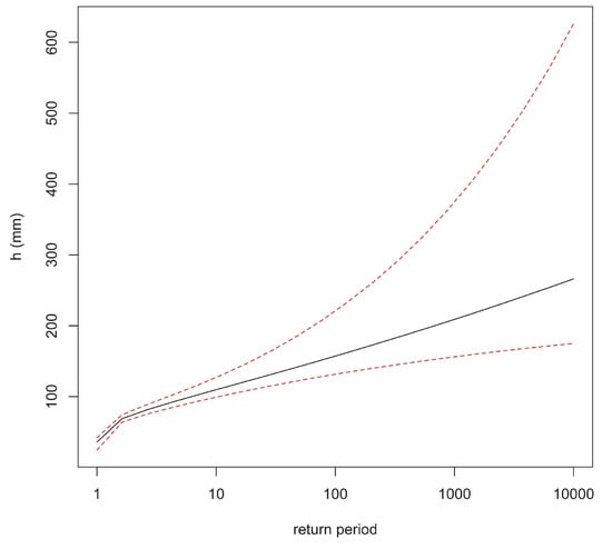
Figure 5.
Posterior return level plot in Bayesian analysis of Dar Es Salaam (TZ) rainfall data: the median (solid line) and the 95% intervals of the posterior probability (dashed lines).
This was due to the heavier upper tail of the posterior distribution (Figure 4), achieved for the non-negative prior on ξ. The summary of Dar Es Salaam (TZ) data is given in Table 2.

Table 2.
Summary of results obtained from different methods of estimation (Dar Es Salaam TZ data).
Moreover, μ was estimated to be 68 mm; nevertheless, MLE returned a lower estimation of the scale parameter σ, with respect to that derived from the Bayesian method. In terms of credibility intervals, the estimation of the shape parameter was more precise using the Bayesian method.
The Bayesian estimates were relatively insensitive to the prior distributions, as shown by the similar parameter and quantile estimates. The computational efforts of the Bayesian approach by using the R software (evdbayes package) were significantly short, requiring very short extra processing time with respect to the MLE. The sole prejudices, in terms of required computational time, regarded both the prior setting up and ensuring that the Markov Chain Monte Carlo had desirable properties. The inclusion of genuine prior information was a compelling factor in favour of the Bayesian inference. This, together with the limited amount of historical data available for the Dar Es Salaam (TZ) analysis, provided significant evidence to prefer the Bayesian analysis instead of the MLE one.
In Figure 6, the autocorrelations for all three parameters after a 5 lag period decreased rapidly. Therefore, it is shown that the result has good mixing.

Figure 6.
Behaviour of autocorrelations for all three parameters of the GEV distribution with lag effects.
Table 3 shows the results of the 3 diagnostics according to the Gelman–Rubin, Geweke and Raftery–Lewis methods, as reported in [34] for checking the convergence of the algorithm. The Gelman–Rubin diagnostic is equal to 1.000 for both μ, σ, and ξ. Therefore, it is known that the chains could be accepted, and this indicates the estimates come from a state space of the parameter, as depicted in Figure 7. In Table 3, Geweke’s test statistics are 0.4307, 0.6353 and 0.9895 for μ, σ and ξ, respectively. Therefore, also in this case, the chain is acceptable, as shown in Figure 8. The last quantitative diagnostic is the Raftery–Lewis method. In Table 3, the dependence factors I are 4.320, 3.860 and 3.85 for μ, σ and ξ, respectively. According to this method, high dependence factors (>5) show significant correlations between estimates, indicating poor mixing. Therefore, the estimated values have good mixing.

Table 3.
Diagnostics by Gelman–Rubin method, Geweke method, and Raftery–Lewis method.

Figure 7.
Gelman plot diagnostic for the three parameters μ, σ, and ξ of Dar Es Salaam (TZ) historical data.

Figure 8.
Geweke plot diagnostic for the three parameters μ, σ, and ξ of Dar Es Salaam (TZ) historical data.
After analyzing the historical data with a stationary approach, the analysis was performed to verify the feasibility of Non-Stationarity data by applying both the GEV and assuming a linear trend for the location parameter.
The GEV log-Likelihood is based on the assumption that the data to be fitted are the observed values of independent random variables X1, …, Xn, where Xi ~ GEV(μ, σ, ξ) for each i = 1, … , n. This assumption can be extended to Xi ~ GEV(μi, σ, ξ), where μi = μ0 + μtrend ti. The parameters (μ, μtrend) are estimated, and the vectors of covariates t = (t1, …, tn) are specified by the user.
In this case study, the MLE fit for the location parameter was = 61.34 + 0.25·ti (where ti = 0, 1, 2, …, 52 years) and associated standard errors were 4.92 and 0.15 for μ0 and μtrend (Figure 9), respectively. The and estimates were 16.22 and 0.071 with standard errors of 1.81 and 0.091, respectively. As shown in Figure 9, this resulted once again in a satisfactory fit. The observed trend of the fitted data with the GEV distribution can be considered a relevant result and suggests further analysis be performed on extended time series with climatic models. An analytic approach to determine the better fit between stationary and Non-Stationary approaches is the Likelihood-Ratio test (eXtremes package [28]). In this test case, the Likelihood-Ratio was equal to about 2.4897, i.e., lower than the 95% quantile of the X12 distribution of 3.8415, suggesting that the covariate ti model did not provide a significant improvement to the model without a covariate. This assumption was also supported by the estimation of the p-value, equal to 0.114.
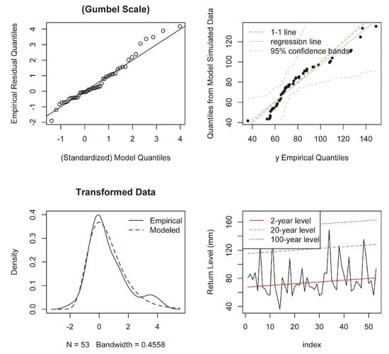
Figure 9.
Observed data fitted with the GEV distribution with a trend.
3.1.2. Historical Data with CMCC Simulation Data
In this section, the analysis is extended by integrating the rainfall observations recorded at Dar Es Salaam (TZ) Airport with the simulated data until year 2050, derived from the climatic forecasting simulations performed by the Euro-Mediterranean Centre for Climate Change (CMCC) for the IPCC scenario RCP8.5, using the COSMO CLM model. Data were downscaled to 1 km spatial precision. Thus, the total dataset was composed of 93 annual maximum rainfall events, 53 observed and 40 simulated data points (Figure 10).
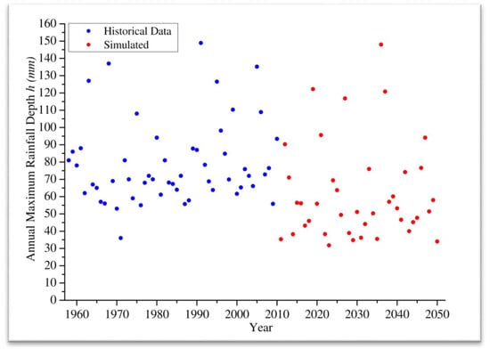
Figure 10.
Annual maximum 24 h rainfall recorded at Dar Es Salaam TZ (1958–2010, blue circles) and simulated by CMCC (2011–2050, red circles).
A similar analysis was performed for the historical data, and the results are summarized in Table 4. For the Bayesian analysis, the MLE was applied as the initial vector θ0 = (, , ) = (59.62, 20.96, −0.00645) by using proposal standard deviations psd = (5.931, 0.193, 0.194). A Markov Chain Monte Carlo (MCMC method) was generated, with a length of 100,000 and good mixing properties. By examining the chain graphically and using the Geweke diagnostic, a burn-in period of very few iterations (about 50) was found to be satisfactory. As in the previous analysis, once a stationary approach was applied, the verification of possible Non-Stationarity of the data was done by using the GEV, as a function of a linear trend for the location parameter. In this case, the MLE fit for the location parameter was = 72.46 − 0.273·ti (where ti = 0, 1, 2, …, 92 years), and associated standard deviations were 3.88 and 0.0683 for μ0 and μtrend, respectively. The and estimations were 18.83 and 0.0542 with associated standard deviations of 1.60 and 0.074, respectively. The Likelihood-ratio was about 13.3543, resulting in a greater 95% quantile of the X12 distribution of 3.8415. The latter suggested that the covariate ti model was a significant improvement over the model without a covariate, obtaining a small p-value of 0.000258.

Table 4.
Summary of results for the different methods of estimation (Dar Es Salaam, TZ).
The posterior return level plot represented in Figure 11 shows once again how the upper 95% interval was farther from the median than the lower one.
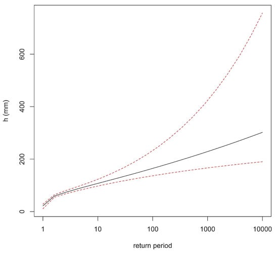
Figure 11.
Posterior return level plot in Bayesian analysis of the Dar Es Salaam (TZ) rainfall data: the median (solid line) and the 95% intervals of the posterior probability (dashed lines).
A naive Bayesian analysis was thus performed, taking near-flat priors that reflected the absence of external information. Indeed, prior on μtrend was a non-informative normal distribution, in a way similar to μ and σ parameters, with a standard deviation of 100. Using MLEs as the initial vector θ0 = (, , , ) = (72.46, 18.83, 0.0542, −0.27), and using proposal standard deviations psd = (5.679, 0.202, 0.187, 0.095), a Markov Chain Monte Carlo (MCMC method) was generated with a length of 100,000 and good mixing properties. As usual, the proposal standard deviation was determined by pilot runs. By examining the chain graphically (Figure 12) and using the Geweke diagnostic plot through the coda package in R [35] (Figure 13), a burn-in period of only 100 iterations was estimated.
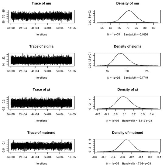
Figure 12.
MCMC realizations of the GEV parameters in a Bayesian Non-Stationary Analysis of Dar Es Salaam (TZ) rainfall data.
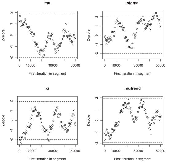
Figure 13.
Geweke plot showing the good properties of the performed chain.
The sample means and standard deviations of each marginal component of the chain were:
whereas the 95% reasonable intervals were [64.14, 79.58], [16.42, 23.15], [−0.0792, 0.211] and [−0.405, −0.129] for μ0, σ, ξ and μtrend, respectively.
In this case, the estimate for the 100-year return level was not feasible because of the linear trend of the location parameter. In Figure 14, the , and return levels are plotted against time from year 1958 to year 2050, as a function of the applied Bayesian analysis. Moreover, the 95% credible intervals are plotted with dashed and dotted lines.
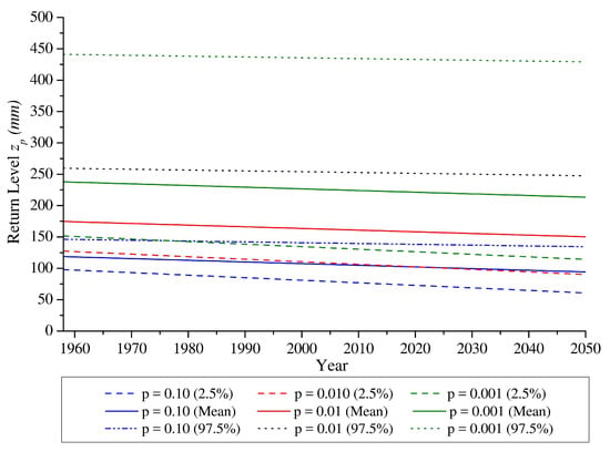
Figure 14.
, and return levels plotted with 95% credible intervals.
In Figure 14, the linear variation over time (although improving the distribution pattern) of the mean parameter was observed, leading towards return level estimations being insignificant over time. As an example, for the 100-year return level, in 1958, 175 mm was achieved with 95% reasonable intervals of [127, 259] mm, becoming 150 mm in 2050 with 95% reasonable intervals of [90, 248] mm. A reduction of only 25 mm was thus observed. In Table 5, the whole set of results for the Non-Stationary Analysis is summarized.

Table 5.
Summary of results for the different methods of estimation (Non-Stationary Analysis, Dar Es Salaam, TZ).
Considering the two methods, the μ0 parameter was estimated to be approximately 72 mm. Nevertheless, as shown in the Maximum Likelihood simulations, it returned a lower estimate of the σ scale parameter than that from the Bayesian method. The estimation of the shape parameter was more precise for the Bayesian method, whereas the estimation of the μtrend parameter was equally precise with both approaches.
3.2. Addis Ababa (ET) Rainfall Data
3.2.1. Historical Data
The second case study regarded the data series of daily rainfall observations recorded at Addis Ababa (ET) Bole, Ethiopia (Latitude: 9.03 N; Longitude: 38.75 E; Elevation: 2354 m a.s.l.), referring to the time span from 1 January 1964 to 31 October 2010. The annual maxima rainfalls are plotted in Figure 15.
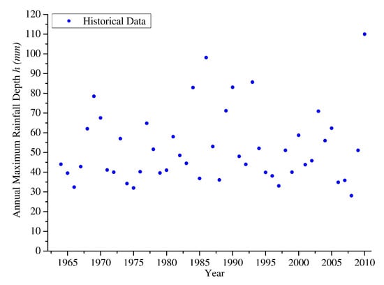
Figure 15.
Annual maximum 24 h rainfalls recorded at Addis Ababa ET (1964–2010).
The same assumptions of the Dar Es Salaam (TZ) case study were applied. Table 6 summarizes the results of the stationary analysis for Addis Ababa (ET).

Table 6.
Summary of results for the different methods of estimation (Addis Ababa, ET).
Similarly to the Bayesian analysis, the same hypotheses were assumed. By using MLEs as initial vector θ0 = (, , ) = (42.76, 11.11, 0.234) and the proposal standard deviations psd = (3.373, 0.323, 0.365), an MCMC method was generated with a length of 100,000, showing satisfactory mixing properties. By examining the chain graphically and using the Geweke diagnostic, a burn-in period of insignificant iterations was found.
The sequence of simulated values (μi, σi, ξi) was transformed, leading towards a sample from the corresponding posterior distribution of the 100-year return level. This gave an estimate = 147.3 mm with 95% credible interval [97, 268] mm. The posterior return level plot represented in Figure 16 shows how the upper 95% interval was farther than the lower interval with respect to the median trend.
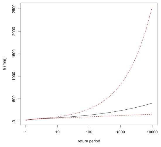
Figure 16.
Posterior return level plot in Bayesian analysis of the Addis Ababa (ET) rainfall data: the median (solid line) and the intervals containing 95% of the posterior probability (dashed lines).
Considering the two methods, μ was estimated to be approximately equal to 43 mm; nevertheless, as confirmed by the Maximum Likelihood simulations, it returned a lower estimate of the scale parameter σ than that from the Bayesian method. The estimation of the shape parameter was more precise for the Bayesian method in terms of the credibility intervals, whilst the opposite was true for the quantile intervals, as a consequence of the greater estimation of ξ parameter.
Once the historical data were analysed with a stationary approach, analysis was also performed to verify a feasible Non-Stationarity of the data, by applying both the GEV and assuming a linear trend for the location parameter. The parameters (μ, μtrend) were estimated, and the vector of covariates t = (t1, …, tn) was specified by the user. In this case, the MLE fit for the location parameter was = 43.67 − 0.047·ti (where ti = 0, 1, 2, …, 52 years) and associated standard errors were 2.58 and 0.088 for μ0 and μtrend, respectively. The and estimate parameters were 10.93 and 0.258, corresponding to associated standard errors of 1.56 and 0.151, respectively. Here again, the Likelihood-ratio was about 0.2575, lower than the 95% quantile of the X12 distribution of 3.8415. This suggested the covariate ti model is not a significant improvement with respect to the model without a covariate. The p-value of 0.612 was in fact estimated.
3.2.2. Historical Data with CMCC Simulation Data
As for the Dar Er Salaam (TZ) case study, the analysis was improved by considering the rainfall observations recorded at Addis Ababa (ET) Bole joined with the simulated data until 2050 performed by Euro-Mediterranean Centre for Climate Change (CMCC) for the IPCC scenario RCP8.5, by using the COSMO CLM model. Data were downscaled to 1 km spatial precision again. Thus, the total dataset contained 87 annual maximum rainfall events: 47 observed and 40 simulated data points (Figure 17).
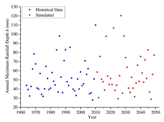
Figure 17.
Annual maximum 24 h rainfalls recorded at Addis Ababa ET (1964–2010, blue circles) and simulated by CMCC (2011–2049, red circles).
The same analysis, already performed for the historical data, was developed, reaching results summarized in Table 7. For the Bayesian analysis, again using MLEs as the initial vector θ0 = (, , ) = (43.93, 12.58, 0.214), and the proposal standard deviations psd = (3.11, 0.206, 0.234), the MCMC method with length 100,000 provided good mixing properties.

Table 7.
A summary of results for the different methods of estimation (Addis Ababa, ET).
The posterior return level plot given in Figure 18 shows that, also in this case, the upper 95% interval was more remote than the lower interval from the median.
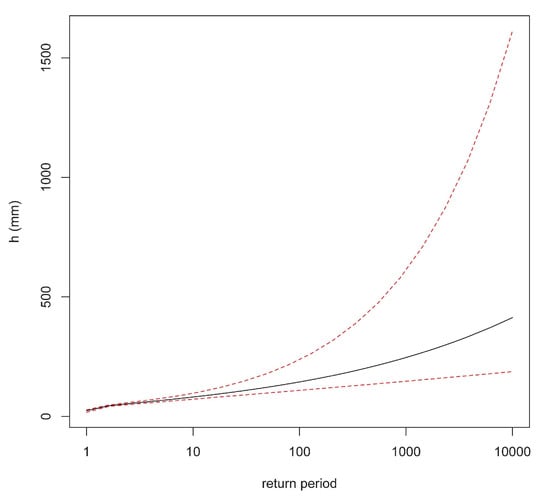
Figure 18.
Posterior return level plot in Bayesian analysis of the Addis Ababa rainfall data: the median (solid line) and the intervals containing 95% of the posterior probability (dashed lines).
Once the data were analysed with a stationary approach, the analysis was devoted to verify a feasible Non-Stationarity of the data, using the GEV as a function of the linear trend for the location parameter. Here, the MLE fit for the location parameter was = 44.02 − 0.00236·ti (where ti = 0, 1, 2, …, 85 years) and associated standard errors were 2.46 and 0.496 for μ0 and μtrend, respectively. The estimates of parameters , and . were 12.57 and 0.216 with associated standard errors of 1.31 and 0.112, respectively. The Likelihood-ratio was about 0.002, i.e., lower than the 95% quantile of the X12 distribution of 3.8415. Thus, the covariate ti model was not able to significantly improve the model without a covariate. The p-value of 0.965 was in fact estimated.
4. Evaluation of Intensity-Duration-Frequency (IDF) Curves
The Intensity-Duration-Frequency (IDF) curves were introduced in hydrology to synthetically define, for a fixed return period T, a generic duration d of a rainfall event and for a given location, information about the maximum rainfall height h and the maximum rainfall intensity i. Through knowledge of these characteristics, synthetic rainfall graphs can be represented, which are useful to reconstruct flood hydrographs.
The analysis was carried out considering the rainfall observations recorded at Dar Es Salaam (TZ) and Addis Ababa (ET), joined with the data until 2050 provided by CMCC for the IPCC Scenario RCP8.5, referring to a downscaling of 1 km spatial precision. The total dataset defined in the previous paragraphs was taken into account.
Generally, IDF curves can be characterized by two or three parameters expressions:
where a(T) and n are the parameters to be estimated through a probabilistic approach.
To define the extreme values in a smaller time steps (10′, 30′, 1 h, 3 h, 6 h, 12 h), the generation of a synthetic sequence of rainfall was required, with statistical properties equal to those for the observed rainfall data. To calculate the extreme values in a smaller time window, the daily rainfall was successively disaggregated by using two models:
- cascade-based disaggregation model
- short-time intensity disaggregation method
These methods have already been validated in Africa [36].
Assuming that daily rainfalls derive from a marked Poisson process, rainfall lag and depths are drawn from exponential Probability Distribution Functions (PDFs) (whose parameters are calculated from the observed rainfall series), using a simple stochastic model, able to describe the occurrence of rainfall as a compound Poisson process with frequency of events λ. The distribution of times τ between precipitation events is an exponential function with mean 1/λ, and exponentially distributed rainfall amounts h with mean γ. This model satisfactory fitted the observed daily rainfall data for individual seasons. Specifically:
- in a cascade-based disaggregation model [37], precipitation data of daily resolution are converted into either 12-hourly, 6-hourly, or 3-hourly values, based on the principles of multiplicative cascade processes. For each year, known γ, λ, it is possible to generate some years of disaggregated values and from these is taken the maximum value for each time window (3 h, 6 h, 12 h);
- in a short-time intensity disaggregation model [38], three fine-resolution time intervals of 1-h, 1/2-h and 10-min are considered.
The , and parameters for the different time steps (10′, 30′, 1 h, 3 h, 6 h, 12 h and 24 h) were evaluated, also considering the 2.5% and 97.5% percentiles, applying a GEV-Bayesian analysis and the zp related to the 100-year return period, calculated through Equation (3).
The IDF curves for T = 100 years for historical data for Dar Es Salaam (TZ) and Addis Ababa (ET) are shown in Figure 19a,b, respectively. In Figure 20a,b IDF curves by combining the historical data and the projected ones are plotted instead. The a and n are summarized in Table 8, with reference to 5, 50, 100 and 500-year return periods.
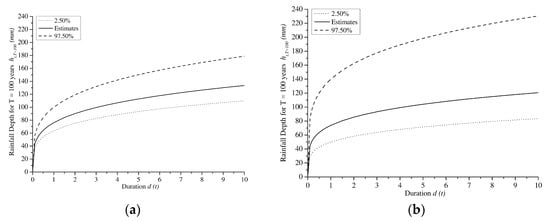
Figure 19.
IDF curves for historical data of: (a) Dar Es Salaam (TZ) and (b) Addis Ababa (ET) cities, with reference to the estimated data (continuous lines), the 2.5% (dotted lines) and 97.5% quantiles (dashed lines).
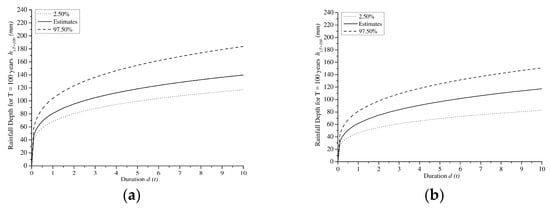
Figure 20.
IDF curves for historical data combined with projected ones of: (a) Dar Es Salaam (TZ) and (b) Addis Ababa (ET) cities, with reference to the estimated data (continuous lines), the 2.5% (dotted lines) and 97.5% quantiles (dashed lines).

Table 8.
IDF parameters from the historical data of Dar Es Salaam (TZ) and Addis Ababa (ET).
From a comparison between Table 8 and Table 9, it was observed that, for the Dar Es Salaam (TZ) case study, similar uncertainties were evaluated from both historical and historical plus projected data. Nevertheless, the IDF derived from the projected data provides greater rainfall intensities values than the historical ones for the whole set of considered durations.

Table 9.
IDF parameters from the historical data combined with projected ones of Dar Es Salaam (TZ) and Addis Ababa (ET).
For Addis Ababa (ET), Table 6 and Table 7 show that the uncertainties estimated from historical data are significantly greater than those derived from historical plus projected ones. This implied less uncertainty in the simulated data. In this case, the IDF derived from the projected data provided greater rainfall intensities than the historical only for durations longer than 16 h.
The Non-Stationary effect, considered in the evaluation with a linear trend of the GEV location parameter, in all the considered situations, i.e., both historical and historical plus projected, did not show significant improvement with respect to the model without a covariate (stationary case).
5. Conclusions
In this paper the effectiveness of the GEV distribution to estimate the annual maxima of rainfall depths is assessed. The shape parameter ξ of such a distribution resulted in the essential parameter to evaluate the properties of extreme value behaviour, namely, the tail of the distribution at its upper end-point.
Estimation of GEV parameters by using methods, such as the Maximum Likelihood, can be unreliable, due to the small length of rainfall records, typically not longer than 30–50 years.
In this study, rainfall data from both Dar Es Salaam (TZ) and Addis Ababa (ET) were analysed, by performing statistical analysis as a function of the 100-year return level.
With regard to Dar Es Salaam (TZ), the confidence intervals for such long return periods were significantly large due to the uncertainty of the extrapolation procedure. With reference to the Addis Ababa (ET) case study, the results were quite different, with a higher shape parameter. In this case, the use of a Bayesian framework to incorporate prior knowledge could improve the estimation reliability by restricting the ξ variation to a physically reasonable range. The Bayesian method showed similar values for the 100-year return level, in spite of wider reasonable intervals at the 95% observed level.
The analysis of the historical data joined with those yielded by the climate model of the CMCC allowed us to estimate the shape parameter with the related standard errors for both test cases.
By applying the Likelihood-ratio test, the Non-Stationary effect was observed for Dar Es Salaam (TZ).
Considering the MLE and Bayesian methods, the μ0 parameter estimated by using the Bayesian method was more precise, whereas the estimation of the μtrend parameter for Dar Es Salaam (TZ) was comparable with both methods.
Results achieved for the two test cases showed that the time series, even though not very numerous, were well represented by stationary GEV. Taking into account additional data from climate models, as a consequence of the sample size increase, the distribution model was forced to be represented by a Non-Stationary GEV.
From these results, it was shown that the Non-Stationary effects are frequently induced by climate models. Indeed, using this trend to analyse the return levels zp, the influence of linear trends in location parameters was observed.
Finally, aiming to answer possible questions about the climate models capability to induce any possible Non-Stationarity in the rainfall series, in future work, further case-studies will be analysed to assess the effectiveness of observed results for different forcing rainfall conditions.
Author Contributions
F.D.P., M.G. and F.N. conceived and performed the statistical analysis; M.G. and A.A. analysed the data; F.P. contributed materials; F.D.P., F.N. and F.P. wrote the paper.
Funding
APC was sponsored by MDPI.
Acknowledgments
In this section you can acknowledge any support given which is not covered by the author contribution or funding sections. This may include administrative and technical support, or donations in kind (e.g., materials used for experiments).
Conflicts of Interest
The authors declare no conflict of interest.
References
- De Paola, F.; Giugni, M.; Topa, M.E.; Bucchignani, E. Intensity-Duration-Frequency (IDF) rainfall curves, for data series and climate projection in African cities. SpringerPlus 2014, 3, 1–18. [Google Scholar] [CrossRef] [PubMed]
- De Risi, R.; Jalayer, F.; De Paola, F.; Iervolino, I.; Giugni, M.; Topa, M.E.; Mbuya, E.; Kyessi, A.; Manfredi, G.; Gasparini, P. Flood Risk Assessment for Informal Settlements. Nat. Hazards 2013, 69, 1003–1032. [Google Scholar] [CrossRef]
- Intergovernmental Panel on Climate Change (IPCC). Climate Change 2007—The Physical Science Basis: Working Group I Contribution to the Fourth Assessment Report of the IPCC; Cambridge University Press: New York, NY, USA, 2007. [Google Scholar]
- Madsen, H.; Lawrence, D.; Lang, M.; Martinkova, M.; Kjeldsen, T.R. Review of trend analysis and climate change projections of extreme precipitation and floods in Europe. J. Hydrol. 2014, 519, 3634–3650. [Google Scholar] [CrossRef]
- Zolina, O. Changes in Intense Precipitation in Europe, Chapter 6. In Changes in Flood Risk in Europe; Kundzewicz, Z.W., Ed.; European Environment Agency Special Publication; IAHS Press: Wallingford, UK, 2012; Volume 10, pp. 97–120. [Google Scholar]
- Gregersen, I.B.; Sørup, H.J.D.; Madsen, H.; Rosbjerg, D.; Mikkelsen, P.S.; Arnbjerg-Nielsen, K. Assessing future climatic changes of rainfall extremes at small spatio-temporal scales. Clim. Chang. 2013, 118, 783–797. [Google Scholar] [CrossRef]
- Jones, M.R.; Fowler, H.J.; Kilsby, C.G.; Blenkinsop, S. An assessment of changes in seasonal and annual extreme rainfall in the UK between 1961 and 2009. Int. J. Climatol. 2013, 33, 1178–1194. [Google Scholar] [CrossRef]
- Van den Bessalar, E.J.M.; Klen-Tank, A.M.G.; Buishand, T.A. Trends in European precipitation extremes over 1951–2010. Int. J. Climatol. 2015, 33, 2682–2689. [Google Scholar] [CrossRef]
- Vasiliades, L.; Galiatsatou, P.; Loukas, A. Nonstationary frequency analysis of annual maximum rainfall using climate covariates. Water Resour. Manag. 2015, 29, 339–358. [Google Scholar] [CrossRef]
- Cheng, L.; AghaKouchak, A. Nonstationary precipitation intensity-duration-frequency curves for infrastructure design in a changing climate. Sci. Rep. 2014, 4, 7093. [Google Scholar] [CrossRef] [PubMed]
- Thiombiano, A.N.; El Adlouni, S.; St-Hilaire, A.; Ouarda, T.B.; El-Jabi, N. Nonstationary frequency analysis of extreme daily precipitation amounts in Southeastern Canada using a peaks-over-threshold approach. Theor. Appl. Climatol. 2017, 129, 413–426. [Google Scholar] [CrossRef]
- Sheikh, M.M.; Manzoor, N.; Ashraf, J.; Adnan, M.; Collins, D.; Hameed, S.; Manton, M.J.; Ahmed, A.U.; Baidya, S.K.; Borgaonkar, H.P. Trends in extreme daily rainfall and temperature indices over South Asia. Int. J. Climatol. 2015, 35, 1625–1637. [Google Scholar] [CrossRef]
- Zilli, M.T.; Carvalho, L.; Liebmann, B.; Silva Dias, M.A. A comprehensive analysis of trends in extreme precipitation over southeastern coast of Brazil. Int. J. Climatol. 2017, 37, 2269–2279. [Google Scholar] [CrossRef]
- Wu, H.; Qian, H. Innovative trend analysis of annual and seasonal rainfall and extreme values in Shaanxi, China, since the 1950s. Int. J. Climatol. 2017, 37, 2582–2592. [Google Scholar] [CrossRef]
- Jenkinson, A.F. The frequency distribution of the annual maximum (or minimum) values of meteorological elements. Q. J. R. Meteorol. Soc. 1955, 81, 158–171. [Google Scholar] [CrossRef]
- Fisher, R.A.; Tippet, L.H.C. Limiting forms of the frequency distribution of the largest or smallest member of a sample. Math. Proc. Camb. Philos. Soc. 1928, 24, 180–190. [Google Scholar] [CrossRef]
- Martins, E.S.; Stedinger, J.R. Generalized maximum-likelihood generalized extreme-value quantile estimators for hydrologic data. Water Resour. Res. 2000, 36, 737–744. [Google Scholar] [CrossRef]
- Coles, S.; Tawn, J.A. A Bayesian Analysis of Extreme Rainfall Data. Appl. Stat. 1996, 45, 463–478. [Google Scholar] [CrossRef]
- De Haan, L.; de Ronde, J. Sea and Wind: Multivariate extremes at work. Extremes 1998, 1, 7–45. [Google Scholar] [CrossRef]
- Geluk, J.L.; de Haan, L.; de Vries, C.G. Weak and Strong Financial Fragility; Tinbergen Institute: Amsterdam, The Netherlands, 2007. [Google Scholar]
- Coles, S. An Introduction to Statistical Modeling of Extreme Values; Springer Series in Statistics; Springer: London, UK, 2001; ISBN 978-1-4471-3675-0. [Google Scholar]
- Cotton, J. Bayesian Priors and Estimation of Extreme Rainfall in Camborne; University of Exeter: Cornwall, UK, 2008. [Google Scholar]
- R Development Core Team. R: A Language and Environment for Statistical Computing; R Foundation for Statistical Computing: Vienna, Austria, 2012; ISBN 3-900051-07-0. [Google Scholar]
- Mailhot, A.; Duchesne, S. Design criteria of urban drainage infrastructures under climate change. J. Water Resour. Plan. Manag. 2009, 136, 201–208. [Google Scholar] [CrossRef]
- Lemmen, D.S.; Warren, F.J.; Lacroix, J.; Bush, E. From Impacts to Adaptation: Canada in a Changing Climate 2007; Government of Canada: Ottawa, ON, Canada, 2008.
- Vincent, L.A.; Mekis, E. Changes in daily and extreme temperature and precipitation indices for Canada over the 20th century. Atmos. Ocean 2006, 44, 177–193. [Google Scholar] [CrossRef]
- Frei, C.; Schöll, R.; Fukutome, S.; Schidli, J.; Vidale, P.L. Future change of precipitation extremes in Europe: Intercomparison of scenarios from regional climate models. J. Geophys. Res. 2006, 111, D06105. [Google Scholar] [CrossRef]
- Gilleland, E.; Katz, R.W. New software to analyse how extremes change over time. Eos Trans. Am. Geophys. Union 2011, 92, 13–14. [Google Scholar] [CrossRef]
- Stephenson, A.G. evd: Extreme Value Distributions. R News 2002, 2, 31–32. [Google Scholar]
- Stephenson, A.; Ribatet, M. Evdbayes: Bayesian Analysis in Extreme Value Theory. R package version 1.1-0. 2012. Available online: http://CRAN.R-project.org/package=evdbayes (accessed on 17 May 2018).
- Koutsoyiannis, D. Statistics of extremes and estimation of extreme rainfall: I. Theoretical investigation. Hydrol. Sci. J. 2004, 49, 575–590. [Google Scholar] [CrossRef]
- Koutsoyiannis, D. Statistics of extremes and estimation of extreme rainfall: II. Empirical investigation of long rainfall records. Hydrol. Sci. J. 2004, 49, 591–610. [Google Scholar] [CrossRef]
- Geweke, J. Evaluating the Accuracy of Sampling-Based Approaches to Calculating Posterior Moments. In Bayesian Statistics; Bernardo, J.M., Berger, J.O., Dawiv, A.P., Smith, A.F.M., Eds.; Clarendon Press: Oxford, UK, 1992; Volume 4. [Google Scholar]
- Lee, C.-E.; Kim, S.U.; Lee, S. Time-dependent reliability analysis using Bayesian MCMC on the reduction of reservoir storage by sedimentation. Stoch. Environ. Res. Risk Assess. 2014, 28, 639–654. [Google Scholar] [CrossRef]
- Plummer, M.; Best, N.; Cowles, K.; Vines, K. Coda: Output Analysis and Diagnostics for MCMC. R package version 0.12-1. 2017. Available online: http://CRAN. R-project. org/package= coda (accessed on 17 May 2018).
- Knoesen, D.; Smithers, J. The development and assessment of a daily rainfall disaggregation model for South Africa. Hydrol. Sci. J. 2009, 54, 217–233. [Google Scholar] [CrossRef]
- Güntner, A.; Olsson, J.; Calver, A.; Gannon, B. Cascade-based disaggregation of continuous rainfall time series: The influence of climate. Hydrol. Earth Syst. Sci. Discuss. 2001, 5, 145–164. [Google Scholar] [CrossRef]
- Connolly, R.D.; Schirmer, J.; Dunn, P.K. A daily rainfall disaggregation model. Agric. For. Meteorol. 1998, 92, 105–117. [Google Scholar] [CrossRef]
© 2018 by the authors. Licensee MDPI, Basel, Switzerland. This article is an open access article distributed under the terms and conditions of the Creative Commons Attribution (CC BY) license (http://creativecommons.org/licenses/by/4.0/).