Estimating Impacts of Agricultural Subsurface Drainage on Evapotranspiration Using the Landsat Imagery-Based METRIC Model


1
Biosystems & Agricultural Engineering Department, Oklahoma State University, Stillwater, OK 74078, USA
2
South Dakota Water Resources Institute, South Dakota State University, Brookings, SD 57007, USA
3
Iowa Soybean Association, Ankeny, IA 50023, USA
4
Agricultural & Biosystems Engineering Department, North Dakota State University, Fargo, ND 58108, USA
*
Author to whom correspondence should be addressed.
Hydrology 2017, 4(4), 49; https://doi.org/10.3390/hydrology4040049
Submission received: 16 October 2017
/
Revised: 30 October 2017
/
Accepted: 6 November 2017
/
Published: 7 November 2017
Abstract
:Agricultural subsurface drainage changes the field hydrology and potentially the amount of water available to the crop by altering the flow path and the rate and timing of water removal. Evapotranspiration (ET) is normally among the largest components of the field water budget, and the changes in ET from the introduction of subsurface drainage are likely to have a greater influence on the overall water yield (surface runoff plus subsurface drainage) from subsurface drained (TD) fields compared to fields without subsurface drainage (UD). To test this hypothesis, we examined the impact of subsurface drainage on ET at two sites located in the Upper Midwest (North Dakota-Site 1 and South Dakota-Site 2) using the Landsat imagery-based METRIC (Mapping Evapotranspiration at high Resolution with Internalized Calibration) model. Site 1 was planted with corn (Zea mays L.) and soybean (Glycine max L.) during the 2009 and 2010 growing seasons, respectively. Site 2 was planted with corn for the 2013 growing season. During the corn growing seasons (2009 and 2013), differences between the total ET from TD and UD fields were less than 5 mm. For the soybean year (2010), ET from the UD field was 10% (53 mm) greater than that from the TD field. During the peak ET period from June to September for all study years, ET differences from TD and UD fields were within 15 mm (<3%). Overall, differences between daily ET from TD and UD fields were not statistically significant (p > 0.05) and showed no consistent relationship.
1. Introduction
Subsurface drainage systems are used to remove standing or excess water from agricultural soils to provide favorable plant growth conditions, improve timeliness of field operations and increase agricultural productivity. Subsurface drained soils are considered some of the most productive soils worldwide [1]. The installation of subsurface drainage systems has continually increased in the U.S. In the late 1980s, about 17% of the U.S. croplands were subsurface drained [2], and this increased to more than 23% in 2012 [3]. Crop Production in many areas of the Corn Belt of the U.S. Upper Midwest would not be possible without subsurface drainage. Installation of subsurface drainage systems changes the flow paths of subsurface water and the rate and timing of water removal from the field altering the soil water balance from the field to the watershed scales.
Among the field water balance components in rainfed crop production, crop water use or evapotranspiration (ET) is generally the second largest component of the water budget after precipitation. Therefore, capturing the ET variations due to installation of subsurface drainage is critical to better understand the impact of subsurface water management practices on agricultural hydrology. In particular, changes in ET affect water yield (the combination of surface runoff and subsurface drainage), which is important for understanding downstream impacts of subsurface drainage systems.
ET shows high variation in space and time. The application of a traditional method for crop ET estimation (ETc) based on crop coefficients (Kc) and reference ET (ETref), where, ETc = Kc × ETref [4], works well; however, this method becomes challenging for representing heterogeneous or larger populations of agricultural fields. Focused efforts over the last several decades in operational satellite-based remote sensing ET models have resulted in accurate estimates of ET and Kc for larger populations of crops and fields [5,6,7,8]. Remotely sensed energy balance (RSEB) models such as SEBAL [9], METRIC [10,11], SEBS [12], ALEXI [13], SSEBop [14] and others are being widely applied to produce spatially distributed ET information at various scales. One of the main advantages of RSEB models is the integration of thermal infrared imagery acquired land surface temperature (LST), which can capture the signals of early vegetation stresses associated with water, nutrient, disease and other stressors.
Previous studies addressing the impact of subsurface drainage on the field water budget have utilized modeling tools [15,16], where ET is estimated using empirical relationships. Konyha et al. [17] applied the field-scale hydrological model DRAINMOD [18] to evaluate the long-term impacts of subsurface drainage on water yield on two different soil types in North Carolina. They reported an increase in annual subsurface flow by 10% and decrease in surface runoff by 66% on more responsive soil (Wasda muck) from improved subsurface drainage (drain tubes), compared to conventional drainage (open field ditches). Several previous studies have shown reduced surface runoff from improved subsurface drainage across the U.S. Midwest [17,19,20], Canada [21,22], Germany [23], and the U.K. [24]. Similarly, recent studies [25,26,27] also reported altered hydrologic responses from agricultural watersheds with artificial subsurface drainage. A study based on eddy covariance tower installed over the fields with and without subsurface drainage in North Dakota (U.S.) reported an increase in ET by 16% and 7% during corn and soybean growing seasons, respectively [28]. At the watershed scale, Yang et al. [29] found a slight decrease in annual cumulative ET from subsurface drainage between 2005 and 2013 in South Dakota, U.S.
While multiple studies have been conducted to study the impact of subsurface drainage on ET at varying scales, very few studies have utilized focused ET modeling using remote sensing techniques. The application of currently available RSEB models and satellite imagery can be utilized to evaluate the localized and seasonal impacts of surface and subsurface water management practices on ET and hydrology. By removing excess water in the spring, subsurface drainage may reduce ET relative to undrained fields during wet spring months, which may affect water availability of crops during summer months. Conversely, establishing a healthier, more vigorous crop through subsurface drainage in the spring, transpiration may be increased during summer months relative to crops in undrained fields that experienced excess water stress in the spring. Landsat imagery with 30 m ground resolution provides a unique opportunity to capture field-scale seasonal ET variations, which is appropriate for the current study. The objective of this study was to examine the impact of subsurface drainage on corn and soybean ET from two fields located in the Upper Midwest of the U.S. using Landsat imagery and the METRIC (Mapping Evapotranspiration at high Resolution with Internalized Calibration) model.
2. Materials and Methods
2.1. Study Sites and Data
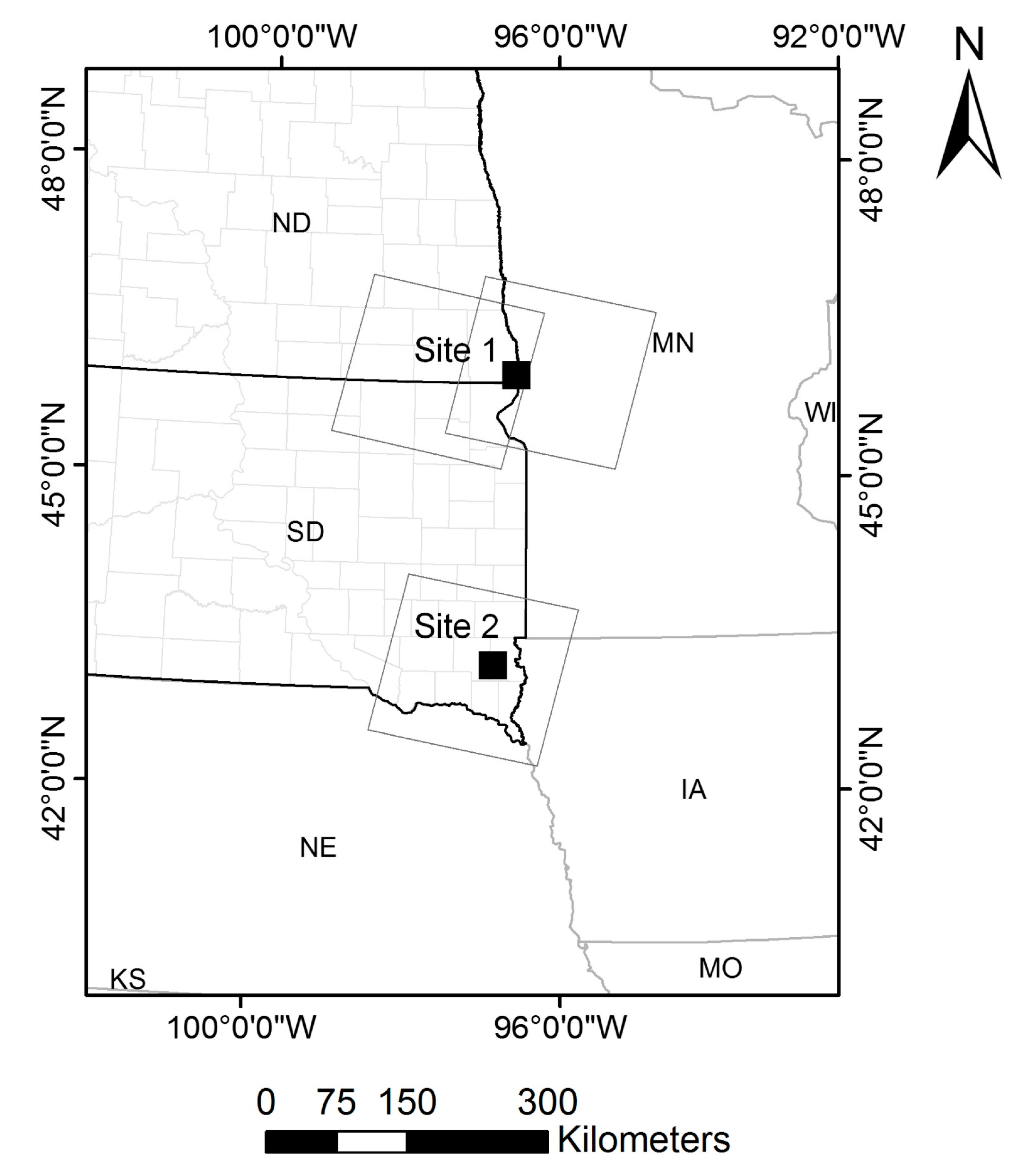
The two study sites were located in Upper Midwest states where subsurface drainage practices are becoming common. Both sites lie within a transitional climate region between the sub-humid Midwest and semiarid Great Plains, and are susceptible to both excess and deficit soil moisture conditions. Site 1 is located in southeast North Dakota (ND), and Site 2 is located in southeast South Dakota (SD) (Figure 1). Site 1 had an area of about 44 ha. and was divided into two equal parts. One-half had a subsurface drain (TD) system installed and the other half had no subsurface drains installed (UD). Site 2 was 28 ha. in size of which 15 ha. was drained (TD) and the remaining area was undrained (UD). A summary of the sites including the study years, crop, soil type and slope and drain system characteristics is provided in Table 1. The study period covered three site-years; 2009 and 2010 at Site 1, and 2013 at Site 2. The crop in years 2009 and 2013 was corn (Zea mays L.), and 2010 was soybean (Glycine max L.). These two sites were selected since they had known areas with and without subsurface drainage, similar soil conditions across the fields, and the same crop and management history between the two treatments.
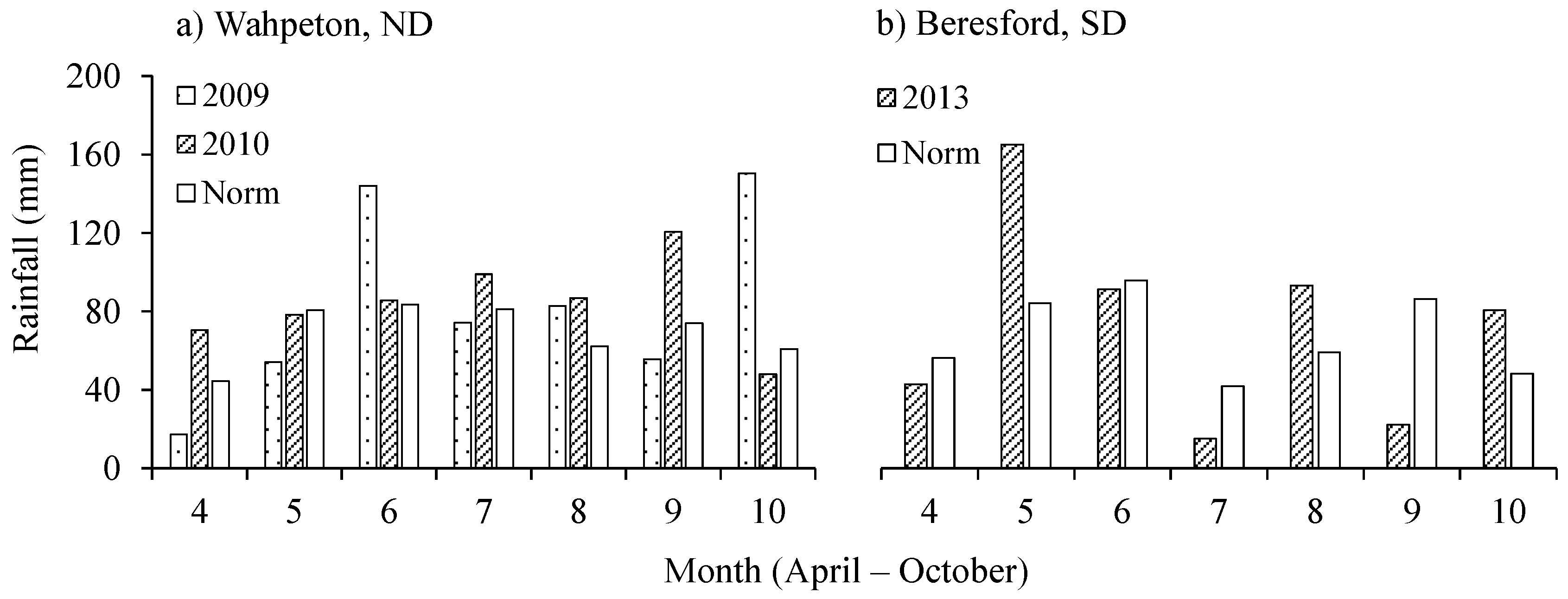
Hourly meteorological information was obtained from the nearest weather station to compute grass-based reference ET (ETo) [30] and necessary inputs for METRIC processing. The North Dakota Agricultural Weather Network (NDAWN) weather station at Wahpeton ND was used at Site 1 and the Automatic Weather Data Network (AWDN) weather station near Beresford, SD, was used for Site 2. The weather data were downloaded from NDAWN (https://ndawn.ndsu.nodak.edu/) and AWDN (http://climate.sdstate.edu/), respectively. The annual rainfall was 579 mm for year 2009 and 590 mm for 2010, which were greater than the normal (1981–2010) rainfall of 568 mm observed at NDAWN Wahpeton station. The AWDN Beresford station received annual rainfall of 510 mm in 2013 which is higher than the normal rainfall of 471 mm. Monthly rainfall distribution during the study years is shown in Figure 2. The average daily air temperature was 4.8 °C in 2009 (highest average was 26.1 °C observed on 14 August) and 6.4 °C (highest average 29.7 °C on 3 July) in 2010 at Wahpeton. Average wind speed was 4.0 m/s and 4.1 m/s for 2009 and 2010, respectively. At the Beresford station, the average daily air temperature was 7.4 °C (highest average was 28.2 °C observed on 25 August) and with average wind speed of 3.8 m/s in 2013.
2.2. METRIC Evapotranspiration
METRIC is a Landsat imagery-based processing model designed to produce high resolution (30 m) ET maps for focused regions less than a few hundred kilometers across [10] and has been widely used over multiple land use types [11,31,32,33,34]. Unlike other RSEB models, METRIC has the advantage of incorporating reference ET from measured weather data for determining the ET conditions at the cold and hot pixel calibration points and for extrapolation of instantaneous to 24-h ET to account for regional advection effects with expected higher accuracy [10]. METRIC requires hourly or shorter meteorological information; this model was selected for our study due to availability of these data and suitability for the purpose of our study at the field scale.
The METRIC model estimates actual ET as a residual of the land surface energy balance as:
where LE is latent heat flux (W/m2), Rn is the net radiation at the surface (W/m2), G is soil heat flux (W/m2), and H is sensible heat flux to the air (W/m2). Other energy balance components such as physical and biochemical energy storage within the crop canopy account for very small percentages of the total energy budget under normal crop growth conditions and are assumed negligible in the model.
LE = Rn − G − H
Rn represents the net energy available at the surface and is computed by subtracting all outgoing radiant fluxes from all incoming radiant fluxes as:
where RSi is incoming shortwave radiation, which includes both direct and diffuse solar radiation flux that reaches the earth surface. RLi is the incoming longwave (thermal) radiation flux originating from the atmosphere, and RLo is outgoing longwave radiation. The surface albedo (α) represents the surface reflectance characteristics and is the ratio of incident radiant flux to reflected radiant flux over the solar spectrum, and εo is broadband surface emissivity. Each of the radiation balance components was estimated as described in [10].
Rn = (1 − α) RSi + RLi − RLo − (1 − εo) RLo
Soil heat flux (G) is heat transmitted to the soil and vegetation by a conduction process. Within METRIC, soil heat flux is calculated as a ratio of G/Rn as:
where LAI is leaf area index (unitless) and was estimated as a function of SAVI (Soil Adjusted Vegetation Index) as described in [10]. Ts is surface temperature (K), estimated by using a modified Plank equation following [35] with atmospheric and surface emissivity correction suggested by [10].
G/Rn = 0.05 + 0.18e−0.521LAI (LAI ≥ 0.5)
G/Rn = 1.80 (Ts − 273.16)/Rn + 0.084 (LAI < 0.5)
H is the rate of heat flux to air by conduction and convection, and it is computed using a one-dimensional, aerodynamic, temperature gradient-based equation of heat transport as:
where ρ is air density (kg/m3), cp is air specific heat capacity (J/kg/K), dT (K) is the temperature difference between two reference heights Z1 and Z2, and rah (s/m) is aerodynamic resistance to heat transport between these two reference heights. The heights Z1 and Z2 float above the canopy with Z1 being 0.1 m and Z2 at 2 m above the zero plane displacement. METRIC utilizes the CIMEC (Calibration using Inverse Modeling of Extreme Conditions) procedure [36] for computation of sensible heat flux. The calibration of H is based on a linear relationship between the dT and Ts [8,36,37,38,39] at two anchor pixels, namely “cold” and “hot” pixels. This inverse calibration process minimizes the need of bias correction of surface temperature (Ts) attributed to atmospheric condition, sensor view angle, or vegetation cover fraction [9,11]. The set of two anchor pixels is selected within the image to represent two extreme conditions of the ET spectrum—a fully vegetated condition where the ET rate is nearing its maximum limit represented by the cold pixel, and a bare, dry soil condition with a lower ET rate is represented by the hot pixel. Cold pixels were selected from densely vegetated areas with NDVI (Normalized Difference Vegetation Index) greater than 0.76 and lower surface temperature (Ts), and hot pixels were selected from a bare soil surface (NDVI < 0.20) with greater Ts values. A bare soil evaporation model (FAO56) [4] was established for the proper adjustment of residual soil evaporation from antecedent rainfall.
H = (ρ × cp × dT)/rah
After computing Rn, G and H, LE is computed as a residual of the surface energy balance using Equation 1. LE is divided by the latent heat of vaporization (λ) to compute ET (mm/hr) at the time of Landsat overpass. Extrapolation of the instantaneous ET (ETinst) at the satellite overpass time to 24-h (daily) ET is based on the reference ET fraction (EToF). EToF is synonymous to the well-known crop coefficient (Kc). Instantaneous EToF was computed as a ratio of ETinst to instantaneous reference ET (ETo), and assumed to be equivalent with 24-h average [11,39]. Additional information about METRIC and processing steps is available in [8,10,11].
Four primary datasets were used for METRIC processing: Landsat imagery, weather information, DEM (digital elevation model) maps, and land-use maps. Altogether, 21 Landsat images were selected for this study (Table 2). These Landsat images were downloaded from the USGS Global Visualization Viewer (http://glovis.usgs.gov/). Hourly weather data collected from the Wahpeton and Beresford weather stations underwent a rigorous quality control procedure [30,40] to identify and remedy the occurrence of unexpected or spurious observations. More information and results from the weather data quality control are available in [41]. DEM information was utilized within the METRIC procedure to account for changes in land surface temperature caused by elevation differences, and land-use maps were used for improving model parameterization and estimation of surface roughness. DEM and land-use maps were obtained from the USGS National Map Viewer (https://viewer.nationalmap.gov/viewer/). The complete METRIC procedure was followed as detailed in [10] with an iterative post-processing data review to confirm the accuracy of the calibration process.
2.3. Monthly and Seasonal ET Estimation
To minimize possible contamination associated with the coarser resolution in the Landsat thermal band, the field edges were buffered 90 m inwards. The 90-m buffer was also maintained when identifying the TD/UD sections of each field site for analysis. After buffering, the TD and UD fields at Site 1 had 132 pixels each. Similarly, the TD and UD fields at Site 2 had 84 pixels each. Daily ET values were estimated on a pixel-by-pixel basis by multiplying daily EToF with daily ETo estimates. Daily ETo values were calculated by summing hourly ETo estimates. The EToF values for days between the selected image dates were interpolated using a cubic spline interpolation [39]. The monthly/seasonal comparisons cover the growing season for soybean (mid-May through September) and corn (mid-May through November).
Allen et al. [8] suggest at least one cloud-free image per month, to generate daily/monthly EToF values. Early in the spring, prior to crop emergence, excessive cloud cover necessitated the creation of a synthetic EToF image representing bare soil conditions based on the soil water balance [4]. However, this procedure was adopted only to produce endpoints for the cubic spline function outside the growing season. Multiple interpolation techniques [42,43,44] have been applied for spatiotemporal coverage for remotely-derived ET products. In this study, monthly and growing season ET were obtained by summing the daily ET values. Statistical analysis of daily and seasonal ET comparisons between TD and UD fields was made by applying Student’s t-test at 95% confidence level.
3. Results
3.1. Comparison of Daily ET
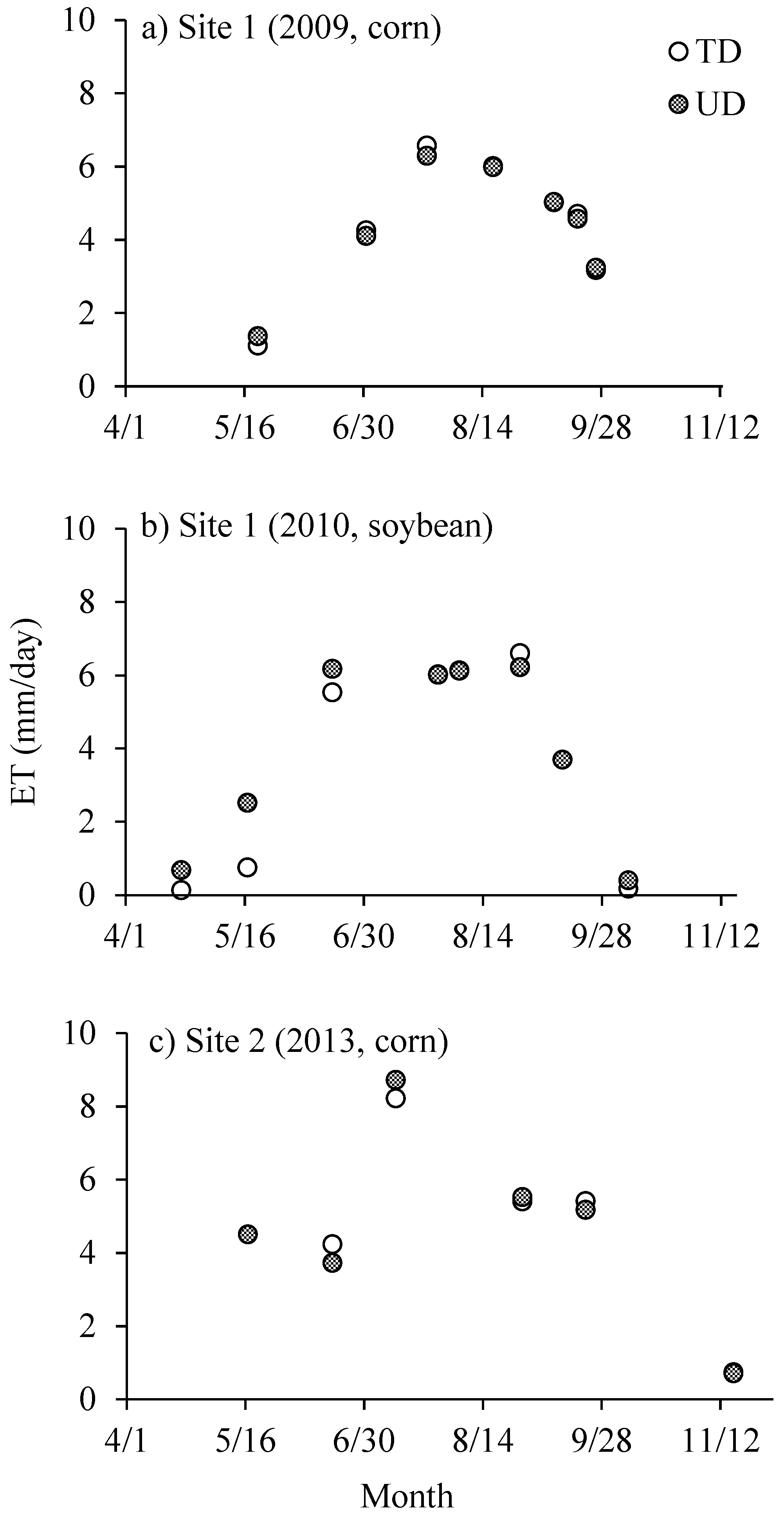
The differences between the daily ET rates from the TD and UD fields were less than 0.55 mm/day (within 20%) for the selected image dates of year 2009 (corn) and 2013 (corn). For the soybean year 2010, the ET difference varied up to 1.76 mm/day (up to 80%). The greater ET differences were observed during the early growing season months (April to June) (Figure 3). For example, the largest ET difference (ET from the UD field greater by 1.76 mm/day; ETo = 5.83 mm/day) was observed on 17 May 2010. Among the selected 21 image dates, the maximum ET (8.72 mm/day; ETo = 7.27 mm/day) was from the UD corn field on 12 July 2013, whereas, the lowest was 0.14 mm/day (ETo = 4.93 mm/day) from the TD soybean field on 22 April 2010. One standard deviation of daily ET for all satellite image dates was within 0.51 mm/day. At Site 1, the maximum one standard deviation was 0.47 mm/day from the UD field on 17 May 2010, whereas, at Site 2, it was 0.51 mm/day from the TD field on 12 July 2013.
The normalized difference vegetation index (NDVI) values of TD field were greater than or equal to the NDVI values from the UD field for all 21 image dates; however, the differences were less than 0.07 (unitless). For the corn years 2009 and 2013, the maximum NDVI value of 0.78 and 0.82 (the same for both TD and UD fields) was observed on the image date 24 July 2009 and 12 July 2013, respectively. For soybean, the maximum NDVI was 0.85 from the TD field (0.83 for UD field) on 28 July 2010. The surface temperature, Ts between the TD and UD fields showed higher variation compared to the NDVI values. The differences between the Ts values were consistent with the differences in ET rates between the TD and UD fields. Greater differences in Ts led to the larger deviations in ET rates. The maximum difference of ET (1.76 mm/day) on 17 May 2010 had a maximum Ts difference of 2.7 K (lower Ts and greater ET from the UD field). A graphic representation of ET variation from the TD and UD fields is shown in Figure 4.
3.2. Monthly and Seasonal ET
The daily ET variations from the TD and UD during the growing seasons are shown in Figure 5. Larger ET differences (TD–UD) were observed during the early growing season for the soybean year 2010 (Figure 5b). For the corn years, daily ET differences were less than 0.60 mm/day (<0.35 mm/day in 2009). During the study period for corn (Figure 5a,c), the differences in total ET between the TD and UD fields were less than 5 mm (2009: UD = 461 mm, TD = 464 mm; 2013: UD = 684 mm, TD = 683 mm). For the soybean year 2010, ET from the UD field (567 mm) was greater than from the TD field (514 mm). However, there was no significant difference (p > 0.05) in daily ET rate between the TD and UD field for all three study years.
Greater daily ET rates were observed from the UD fields during the early growing season (mid-May to mid-June) for year 2010; however, for 2009 and 2013, ET rates from the TD and UD fields were similar during this same season (Figure 5). The monthly ET variation between TD and UD fields was within 10 mm for all study months except for May (39 mm) and June (16 mm) in 2010 (Figure 6). The greater ET differences in May and June 2010 are potentially associated with accumulation of soil moisture in the UD field due to rainfall and snow melted runoff water before the growing season (Figure 2). During April 2010, 75 mm rainfall was measured which is 30 mm above the normal rainfall (Figure 2).
The maximum monthly EToF values during the corn years were observed in August. In 2009, EToF values reached a maximum of 1.19 from TD fields and 1.18 from the UD field. In 2013, the maximum EToF value was 1.16 in the UD field and 1.11 in the TD field. Similar to the corn study years, the maximum EToF value of soybean was also in August, at 1.11 and 1.08 for TD and UD, respectively. These results indicate that the August month has a greater potential of ET rates for both corn and soybean plants when provided with sufficient soil moisture.
The greatest monthly ETo occurred in July during all study years (Figure 6). June was the month after July with the greatest ETo. Therefore, June–July (JJ) were the months with highest atmospheric water demand (ETo). However, the highest corn and soybean ET was observed in July–August (JA) months. During the greatest ETo months (JJ), ET was greater from the TD field for corn years and from the UD field for soybean years (Table 3). Similarly, during the greatest ET months (JA), ET from the TD field was greater for 2009 and 2010, and lower for 2013. The bi-monthly (JJ,JA,AS) ET differences between TD and UD fields were within 7 mm except for JJ-2010 (18 mm) and JA-2013 (16 mm) (Table 3). The differences between ET from TD and UD fields during these bi-monthly periods were not significant (p > 0.05). June–September (JJAS) rainfall accounted for less than 60% of actual ET, indicating the deficit crop water supplied either by accumulated soil moisture from the early growing season rainfall or from the shallow water table. Total ETo during JJAS was greater than actual ET at Site 1; however, it was lower at Site 2 for the same time-period (Table 3).
4. Discussion
Satellite- and/or air-borne imagery is continuously applied for multiple applications as they can provide spatially distributed information at varying scales. Higher ground-resolution Landsat images (30 m) are useful for wide areas of agricultural monitoring such as crop health, crop water use, and stresses associated with climate. The METRIC model, primarily developed for estimating water use (ET) from the agricultural crops, was applied to estimate ET from the subsurface drained and undrained corn/soybean fields in this study. The model successfully captured the field-scale ET variations attributed to subsurface drained/undrained water management practices. As METRIC was applied during the growing season at the agricultural regions of southeast North Dakota and South Dakota, there were not any observed challenges such as selection of appropriate anchor pixels that potentially obstruct the successful processing of the METRIC model. However, during the early and late growing season, there were difficulties in obtaining sufficient cloud-free images. Due to this reason, the 2009 study was reduced to a shorter period (Figure 5a) compared to the total corn growing season.
The results showed no significant difference (p > 0.05) of the ET rates from the TD and UD fields. Differences on daily ET rates were greater during the early growing season than those of later seasons (Figure 5), which is potentially linked to more rainfall during the early growing season months (Figure 2) so that there is greater soil moisture difference between TD and UD fields. During the period of June to September (JJAS), total ET from the TD and UD field was within a 15 mm (<3%) difference. JJAS are the months with the greatest ET rates during the growing seasons for corn and soybeans. Although there were greater variations in rainfall during JJAS (Figure 2), ET differences between TD and UD fields were low (Figure 6). These rainfall and ET patterns from our study indicate that the subsurface drainage has no significant (p > 0.05) impact on corn/soybean ET during the JJAS period. However, the larger variations between subsurface drained and undrained fields may be observed during the other months/seasons when there is significant variation in soil moisture conditions. The greater amount of actual ET compared to rainfall during JJAS (including summer months June to August) signifies the lower likelihood of gravitational water in the soil profile draining out through the subsurface drainage. The lower availability of soil moisture to flow through subsurface drainage during summer is also reported in previous studies [45,46] compared to other season months. The greater impact of subsurface drainage on subsurface flow was found in the late spring to early summer (March–June) months compared to other season months [15,25], indicating high soil moisture variation during these seasons. These previous studies and results from our study indicate that subsurface drainage impact on ET (and subsurface flow) is primarily associated with the soil moisture availability within a certain time period of a year. Beside soil moisture, soil type and crop characteristics, land topography [47], and drainage designs [15,46] can impact soil moisture availability in the crop root zone and crop water use behavior, which ultimately impact water budgets from a field to larger scales.
The findings of the current study are in agreement with previous field-scale studies [15,16,28] evaluating the impact of subsurface drainage on ET. For example, Rijal et al. [28] reported higher ET from the drained field by 16% and 7% during the corn and soybean growing season, respectively. In comparison to our study, a similar result of greater ET from the TD field was observed for year 2009; however, our results were different for the 2010. Rijal et al. [28] study covered the timespan between planting and date of harvest, while our study was dependent on the availability of cloud-free Landsat imagery for METRIC processing, which resulted in the variation in coverage of study periods. Similarly, Youssef et al. [16] also found less impact (5% increase) of subsurface drainage water management on annual ET. While these studies used hydrological modeling and field-measurement approaches, our study applied the remote sensing method. All of these methods have their own advantages and limitations. A comparison of daily ET estimates using METRIC and EC measurements at Site 1 (2009) showed lower normalized difference in ET rates between TD and UD fields from METRIC (10%) compared to EC measurements (18%) [48]. The potential sources of errors and uncertainties associated with these ET estimation methods are also discussed in [48]. METRIC uses the canopy temperature as the primary indicator of ET. The canopy temperature responds immediately to changes in crop water use due to evaporative cooling. Even subtle changes in water use from, e.g., drainage system impacts, irrigation or differences in soil moisture content, are quantified. An example of the sensitivity to subtle changes is in Figure 4, where within-field variation is ET is apparent. In addition, the comparisons between TD and UD are made side-by-side within the same images (as opposed to comparisons of fields from different images) which reduces the risk and magnitude of uncertainty in the ET estimates. A detailed description on ET estimation methods, sources of errors and uncertainties is presented in [49]. Typical errors from remotely sensed energy balance models are within 30% [7,49] with greater accuracy on seasonal estimates [6].
ET estimation within the METRIC model is driven by the selection of anchor pixels. The selection of appropriate anchor pixels is based on professional judgment of the individual applying the model [10]. In this study, our best judgment was used during the selection of anchor pixels with an iterative post-processing data review to confirm the accuracy of the calibration process. An explanation on the impact of the anchor pixel section on ET with respect to the size of the study area, spatial resolution and quality of the imagery is presented in [50]. For example, finding a suitable cold pixel within an image during low vegetation conditions (NDVI < 0.75) may become problematic during the non-growing season. However, an alternative approach may be applied as described by [10,32,51] to complete the image processing using the METRIC model. Application of the METRIC model may not be appropriate when high-quality hourly or shorter time interval meteorological data is not available. Similar to other RSEB models, the need of cloud-free satellite images may also hinder successful image processing using the METRIC model.
Studies on the impacts of agricultural water management practices on each of the water balance components are crucial from a field scale to larger scales. These studies are important to understand whether altered hydrologic responses from agricultural watersheds are linked with climate [52,53] and/or with water management practices [54]. Our study analyzed the interactions between subsurface drainage and ET at the field scale for three growing seasons across similar climatic zones. The study needs to be extended to cover multiple years and more locations to encompass the local climatic variations. Further, the Landsat-based METRIC ET products can be integrated with aerial photograph-detected subsurface drainage systems [55] to precisely evaluate ET impacts at larger scales.
5. Conclusions
This study was conducted to estimate and analyze the impact of subsurface drainage water management on evapotranspiration at the field scale. The Landsat imagery-based METRIC model was applied to estimate and compare ET from subsurface drained (TD) and undrained (UD) fields during selected study years of corn and soybean growing seasons. The two study sites were located in southeast North Dakota (Site 1, year 2009 and 2010) and southeast South Dakota (Site 2, year 2013). Results indicated greater daily ET rates from the UD fields than from the TD fields during the early growing season for the selected satellite image dates (Table 2, Figure 2) at both sites. The differences between ET from TD and UD fields were within 10% and were not significant (p > 0.05) during the study period. The ET differences during June–September (JJAS) were less than 3% (less than 15 mm). The study found no consistent relationship in variation in ET rates incurred by the installation of a subsurface drainage system. However, it may vary during non-growing seasons based on soil and crop characteristics, subsurface drainage system designs, local climate or other impacting factors. The Landsat imagery-based METRIC model successfully captured the variations in ET on a field-by-field basis and can be applied when high-resolution ET maps are needed.
Acknowledgments
The funding for the project was provided by the South Dakota Water Resources Institute in collaboration with USGS National Institutes for Water Resources. The research study was supported by the South Dakota Automated Agricultural Data Network, North Dakota Agricultural Weather Network (NDAWN), AmericaView and the South Dakota Agricultural Experiment Station.
Author Contributions
Christopher Hay designed the study. Kul Khand and Jeppe Kjaersgaard prepared and processed the data. Kul Khand, Jeppe Kjaersgaard and Christopher Hay contributed to the analyses, interpretation of results and wrote the paper, and Xinhua Jia revised it.
Conflicts of Interest
The authors declare no conflict of interest.
References
- Skaggs, R.W.; Breve, M.A.; Gilliam, J.W. Hydrologic and water quality impacts of agricultural drainage. Crit. Rev. Environ. Sci. Technol. 1994, 24, 1–32. [Google Scholar] [CrossRef]
- Pavelis, G.A. Farm Drainage in the United States: History, Status, and Prospects; United States Department of Agriculture, Economic Research Service: Washington, DC, USA, 1987. [Google Scholar]
- Natural Resources Conservations Service—Web Soil Survey. Available online: http://websoilsurvey.nrcs.usda.gov/app/HomePage.htm (accessed on 8 May 2014).
- Allen, R.G.; Pereira, L.S.; Raes, D.; Smith, M. Crop Evapotranspiration—Guidelines for Computing Crop Water Requirements—FAO Irrigation and Drainage Paper 56; Food and Agriculture Organization of the United Nations: Rome, Italy, 1998. [Google Scholar]
- Tasumi, M.; Allen, R.G.; Trezza, R.; Wright, J.L. Satellite-Based Energy Balance to Assess within-Population Variance of Crop Coefficient Curves. J. Irrig. Drain. Eng. 2005, 131, 94–109. [Google Scholar] [CrossRef]
- Gowda, P.H.; Chavez, J.L.; Colaizzi, P.D.; Evett, S.R.; Howell, T.A.; Tolk, J.A. Remote sensing based energy balance algorithms for mapping ET: Current status and future challenges. Trans. Am. Soc. Agric. Biol. Eng. 2007, 5, 1639–1644. [Google Scholar]
- Kalma, J.D.; McVicar, T.R.; McCabe, M.F. Estimating Land Surface Evaporation: A Review of Methods Using Remotely Sensed Surface Temperature Data. Surv. Geophys. 2008, 29, 421–469. [Google Scholar] [CrossRef]
- Allen, R.; Irmak, A.; Trezza, R.; Hendrickx, J.M.H.; Bastiaanssen, W.; Kjaersgaard, J. Satellite-based ET estimation in agriculture using SEBAL and METRIC. Hydrol. Process. 2011, 25, 4011–4027. [Google Scholar] [CrossRef]
- Bastiaanssen, W.G.M. Regionalization of Surface Flux Densities and Moisture Indicators in Composite Terrain: A Remote Sensing Approach under Clear Skies in Mediterranean Cimates. Ph.D. Thesis, CIP Data Koninklijke Bibliotheek, Den Haag, The Netherlands, 1995. [Google Scholar]
- Allen, R.G.; Tasumi, M.; Trezza, R. Satellite-based energy balance for mapping evapotranspiration with internalized calibration (METRIC)—Model. J. Irrig. Drain. Eng. 2007, 133, 380–394. [Google Scholar] [CrossRef]
- Allen, R.G.; Tasumi, M.; Morse, A.; Trezza, R.; Wright, J.L.; Bastiaansseen, W.; Kramber, W.; Lorite, I.; Robison, C. Satellite-based energy balance for mapping evapotranspiration with internalized calibration (METRIC)–Applications. J. Irrig. Drain. Eng. 2007, 133, 395–406. [Google Scholar] [CrossRef]
- Su, Z. The surface energy balance systems (SEBS) for estimation of turbulent fluxes. Hydrol. Earth Syst. Sci. 2002, 6, 85–99. [Google Scholar] [CrossRef]
- Anderson, M.C.; Norman, J.M; Diak, G.R.; Kustas, W.P.; Mecikalski, J.R. A two-source time-integrated model for estimating surface fluxes using thermal infrared remote sensing. Remote Sens. Environ. 1997, 60, 195–216. [Google Scholar] [CrossRef]
- Senay, G.B.; Bohms, S.; Singh, R.K.; Gowda, P.H.; Velpuri, N.M.; Alemu, H.; Verdin, J.P. Operational evapotranspiration mapping using remote sensing and weather datasets: A new parameterization for the SSEB approach. J. Am. Water Resour. Assoc. 2013, 49, 577–591. [Google Scholar] [CrossRef]
- Jin, C.-X.; Sands, G.R. The Long–Term Field–Scale Hydrology of Subsurface Drainage Systems in a Cold Climate. Trans. Am. Soc. Agric. Biol. Eng. 2003, 46, 1011–1021. [Google Scholar]
- Youssef, M.A.; Skaggs, R.W.; Kelly, R.T.; Ahmed, M.A.; Jaynes, D.B. Drainmod-Simulated Performance of Drainage Water Management across the U.S. Midwest. In Proceedings of the 9th International Drainage Symposium Held Jointly with CIGR and CSBE/SCGAB, St. Joseph, MI, USA, 13–16 June 2010; ASABE: St. Joseph, MI, USA, 2010. [Google Scholar]
- Konyha, K.D.; Skaggs, R.W.; Gilliam, J.W. Effects of drainage and water-management practices on hydrology. J. Irrig. Drain. Eng. 1992, 118, 807–819. [Google Scholar] [CrossRef]
- Skaggs, R.W. A Water Management Model for Shallow Water Table Soils; Water Resources Research Institute of the University of North Carolina Report 134; Water Resources Research Institute of the University of North Carolina: Raleigh, NC, USA, 1978. [Google Scholar]
- Bottcher, A.B.; Monke, E.J.; Huggins, L.F. Nutrient and sediment loadings from a subsurface drainage system. Trans. Am. Soc. Agric. Eng. 1981, 24, 1221–1226. [Google Scholar] [CrossRef]
- Skaggs, R.W.; Gilliam, J.W. Effect of drainage system design and operation on nitrate transport. Trans. Am. Soc. Agric. Eng. 1981, 24, 929–934. [Google Scholar] [CrossRef]
- Irwin, R.W.; Whiteley, H.R. Effects of land drainage on stream flow. Can. Water Resour. J. 1983, 8, 88–103. [Google Scholar] [CrossRef]
- Whiteley, H.R.; Ghate, S.R. Sources and amounts of overland runoff from rain on three small watersheds. Can. Agric. Eng. 1979, 21, 1–7. [Google Scholar]
- Baden, W.; Eggelsman, R. The hydrologic budget of the highbogs in the Atlantic region. In Proceedings of the Third International Peat Congress, Quebec, QC, Canada, 18–23 August 1968. [Google Scholar]
- Robinson, M. Impact of Improved Land Drainage on River Flows; Institute of Hydrology: Wallingford, Oxon, UK, 1990. [Google Scholar]
- Schilling, K.E.; Helmers, M. Effects of subsurface drainage tiles on streamflow in Iowa agricultural watersheds: Exploratory hydrograph analysis. Hydrol. Process. 2008, 22, 4497–4506. [Google Scholar] [CrossRef]
- Rahman, M.M.; Lin, Z.; Jia, X.; Steele, D.D.; DeSutter, T.M. Impact of subsurface drainage on streamflows in the Red River of the North basin. J. Hydrol. 2014, 511, 474–483. [Google Scholar] [CrossRef]
- Hoogestraat, G.K.; Stamm, J.F. Climate and Streamflow Characteristics for Selected Streamgages in Eastern South Dakota, Water Years 1945–2013; United States Geological Survey Scientific Investigations Report 2015-5146; U.S. Geological Survey: Reston, VA, USA, 2015. [Google Scholar]
- Rijal, I.; Jia, X.; Zhang, X.; Steele, D.D.; Scherer, T.F.; Akyuz, A. Effects of Subsurface Drainage on Evapotranspiration for Corn and Soybean Crops in Southeastern North Dakota. J. Irrig. Drain. Eng. 2012, 138, 1060–1067. [Google Scholar] [CrossRef]
- Yang, Y.; Anderson, M.; Gao, F; Hain, C.; Kustas, W.; Meyers, T.; Crow, W.; Finocchiaro, R.; Sun, L.; Yang, Y. Impact of Tile Drainage on Evapotranspiration in South Dakota, USA, Based on High Spatiotemporal Resolution Evapotranspiration Time Series from a Multisatellite Data Fusion System. IEEE J.-STARS 2017, 10, 2550–2564. [Google Scholar] [CrossRef]
- Environmental and Water Resources Institute of the American Society of Civil Engineers (ASCE-EWRI). The ASCE Standardized Reference Evapotranspiration Equation; Report of the ASCE-EWRI Task Committee on Standardization of Reference Evapotranspiration; ASCE: Reston, VA, USA, 2005. [Google Scholar]
- Santos, C.; Lorite, I.J.; Allen, R.G.; Tasumi, M. Aerodynamic Parameterization of the Satellite-Based Energy Balance (METRIC) Model for ET Estimation in Rainfed Olive Orchards of Andalusia, Spain. Water Resour. Manag. 2012, 26, 3267–3283. [Google Scholar] [CrossRef]
- Trezza, R.; Allen, R.G.; Tasumi, M. Estimation of actual evapotranspiration along the Middle Rio Grande of New Mexico using MODIS and Landsat imagery with the METRIC model. Remote Sens. 2013, 5, 5397–5423. [Google Scholar] [CrossRef]
- Bhattarai, N.; Shaw, S.B.; Quackenbush, L.J.; Im, J.; Niraula, R. Evaluating five remote sensing based single-source surface energy balance models for estimating daily evapotranspiration in a humid subtropical climate. Int. J. Appl. Earth Obs. Geoinf. 2016, 49, 75–86. [Google Scholar] [CrossRef]
- Numata, I.; Khand, K.; Kjaersgaard, J.; Cochrane, MA.; Silva, S.S. Evaluation of Landsat-Based METRIC Modeling to Provide High-Spatial Resolution Evapotranspiration Estimates for Amazonian Forests. Remote Sens. 2017, 9, 46. [Google Scholar] [CrossRef]
- Markham, B.L.; Barker, J.L. Landsat MSS and TM Postcalibration Dynamic Ranges, Exoatmospheric Reflectances and at-Satellite Temperatures; Earth Observation Satellite Company Landsat Technical Notes 1; EOSAT: Lanham, MD, USA, 1986. [Google Scholar]
- Bastiaanssen, W.G.M.; Menenti, M.; Feddes, R.A.; Holtslag, A.A.M. A Remote Sensing Surface Energy Balance Algorithm for Land (SEBAL). 1. Formulation. J. Hydrol. 1998, 212, 198–212. [Google Scholar] [CrossRef]
- Franks, S.W.; Beven, K.J. Conditioning a Multiple-Patch SVAT Model Using Uncertain Time-Space Estimates of Latent Heat Fluxes as Inferred from Remotely Sensed Data. Water Resour. Res. 1999, 35, 2751–2761. [Google Scholar] [CrossRef]
- Jacob, F.; Olioso, A.; Gu, X.F.; Su, Z.; Seguin, B. Mapping surface fluxes using airborne visible, near infrared, thermal infrared remote sensing data and a spatialized surface energy balance model. Agronomie 2002, 22, 669–680. [Google Scholar] [CrossRef]
- Kjaersgaard, J.; Allen, R.G.; Irmak, A. Improved Methods for Estimating Monthly and Growing Season ET Using METRIC Applied to Moderate Resolution Satellite Imagery. Hydrol. Process. 2011, 25, 4028–4036. [Google Scholar] [CrossRef]
- Kjaersgaard, J.; Allen, R.G. Remote Sensing Technology to Produce Consumptive Water Use Maps for the Nebraska Panhandle; University of Idaho Kimberley R & E Center Research Completion Report; University of Idaho Kimberley R & E Center: Kimberly, ID, USA, 2010. [Google Scholar]
- Khand, K. Estimating Impacts of Subsurface Drainage on Evapotranspiration Using Remote Sensing. Master’s Thesis, South Dakota State University, Brookings, SD, USA, 2014. [Google Scholar]
- Long, D.; Singh, V.P. Integration of the GG model with SEBAL to produce time series of evapotranspiration of high spatial resolution at watershed scales. J. Geophys. Res. Atmos. 2010, 115, D21128. [Google Scholar] [CrossRef]
- Dhungel, R.; Allen, R.G.; Trezza, R.; Robison, C.W. Evapotranspiration between satellite overpasses: Methodology and case study in agricultural dominant semi-arid areas. Meteorol. Appl. 2016, 23, 714–730. [Google Scholar] [CrossRef]
- Cammalleri, C.; Anderson, M.C.; Gao, F.; Hain, C.R.; Kustas, W.P. Mapping daily evapotranspiration at field scales over rainfed and irrigated agricultural areas using remote sensing data fusion. Agric. For. Meteorol. 2014, 186, 1–11. [Google Scholar] [CrossRef]
- King, K.W.; Fausey, N.R.; Williams, M.R. Effect of subsurface drainage on streamflow in an agricultural headwater watershed. J. Hydrol. 2014, 519, 438–445. [Google Scholar] [CrossRef]
- Singh, R.; Helmers, M.J.; Crumpton, W.G.; Lemke, D.W. Predicting effects of drainage water management in Iowa’s subsurface drained landscapes. Agric. Water Manag. 2007, 92, 162–170. [Google Scholar] [CrossRef]
- Turunen, M.; Warsta, L.; Paasonen-Kivekäs, M.; Nurminen, J.; Myllys, M.; Alakukku, L.; Äijö, H.; Puustinen, M.; Koivusalo, H. Modeling water balance and effects of different subsurface drainage methods on water outflow components in a clayey agricultural field in boreal conditions. Agric. Water Manag. 2013, 121, 135–148. [Google Scholar] [CrossRef]
- Kjaersgaard, J.; Khand, K.; Hay, C.; Jia, X. Estimating Evapotranspiration from Fields with and without Tile Drainage Using Remote Sensing. In Proceedings of the World Environmental and Water Resources Congress, Portland, OR, USA, 1–5 June 2014; Wayne, C.H., Ed.; ASCE: Reston, VA, USA, 2014. [Google Scholar]
- Allen, R.G.; Pereira, L.S.; Howell, T.A.; Jensen, M.E. Evapotranspiration information reporting: I. Factors governing measurement accuracy. Agric. Water Manag. 2011, 98, 899–920. [Google Scholar] [CrossRef]
- Long, D.; Singh, V.P. Assessing the impact of end-member selection on the accuracy of satellite-based spatial variability models for actual evapotranspiration estimation. Water Resour. Res. 2013, 49, 2601–2618. [Google Scholar] [CrossRef]
- Khand, K.; Numata, I.; Kjaersgaard, J.; Vourlitis, G.L. Dry Season Evapotranspiration Dynamics over Human-Impacted Landscapes in the Southern Amazon Using the Landsat-Based METRIC Model. Remote Sens. 2017, 9, 706. [Google Scholar] [CrossRef]
- Singh, R.; Helmers, M.J.; Kaleita, A.L.; Takle, E.S. Potential impact of climate change on subsurface drainage in Iowa’s subsurface drained landscapes. J. Irrig. Drain. Eng. 2009, 135, 459–466. [Google Scholar] [CrossRef]
- Gupta, S.C.; Kessler, A.C.; Brown, M.K.; Zvomuya, F. Climate and agricultural land use change impacts on streamflow in the upper midwestern United States. Water Resour. Res. 2015, 51, 5301–5317. [Google Scholar] [CrossRef]
- Schottler, S.P.; Ulrich, J.; Belmont, P.; Moore, R.; Lauer, J.; Engstrom, D.R.; Almendinger, J.E. Twentieth Century Agricultural Drainage Creates More Erosive Rivers. Hydrol. Process. 2014, 28, 1951–1961. [Google Scholar] [CrossRef]
- Naz, B.S.; Ale, S.; Bowling, L.C. Detecting subsurface drainage systems and estimating drain spacing in intensively managed agricultural landscapes. Agric. Water Manag. 2009, 96, 627–637. [Google Scholar] [CrossRef]
Figure 1.
Location of the study sites in North Dakota (ND, Site 1) and South Dakota (SD, Site 2). Inclined rectangle shapes represent Landsat path/row over Site 1 (29/28 and 30/28) and Site 2 (29/30).
Figure 1.
Location of the study sites in North Dakota (ND, Site 1) and South Dakota (SD, Site 2). Inclined rectangle shapes represent Landsat path/row over Site 1 (29/28 and 30/28) and Site 2 (29/30).

Figure 2.
Monthly rainfall observed at the (a) Wahpeton (North Dakota) and (b) Beresford (South Dakota) weather station during the study years, and the normal rainfall (1980–2010).
Figure 2.
Monthly rainfall observed at the (a) Wahpeton (North Dakota) and (b) Beresford (South Dakota) weather station during the study years, and the normal rainfall (1980–2010).

Figure 3.
Comparison of daily evapotranspiration (ET) rates from the subsurface drained (TD) and undrained (UD) corn (a,c) and soybean (b) fields at satellite overpass dates.
Figure 3.
Comparison of daily evapotranspiration (ET) rates from the subsurface drained (TD) and undrained (UD) corn (a,c) and soybean (b) fields at satellite overpass dates.

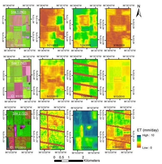
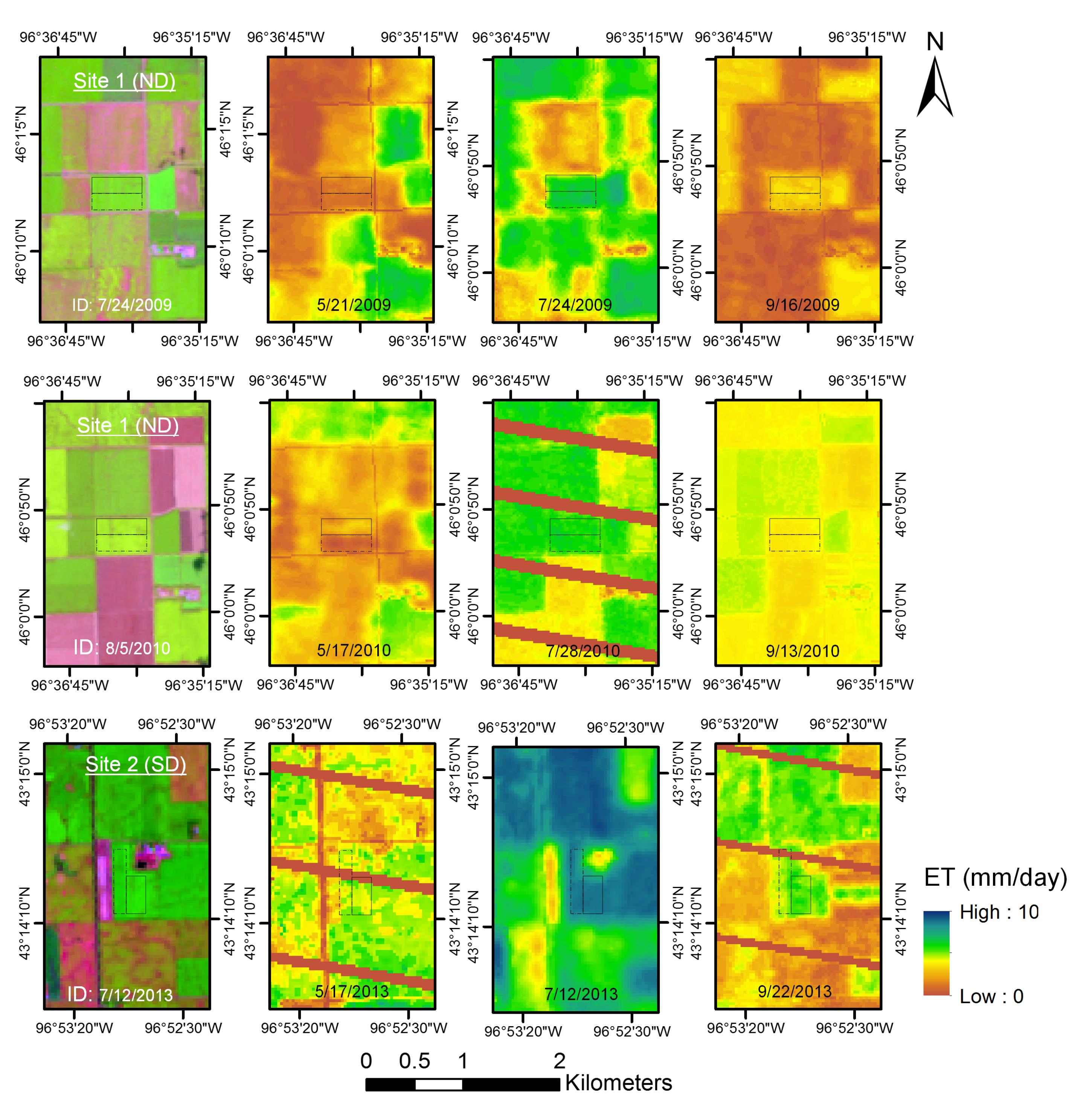
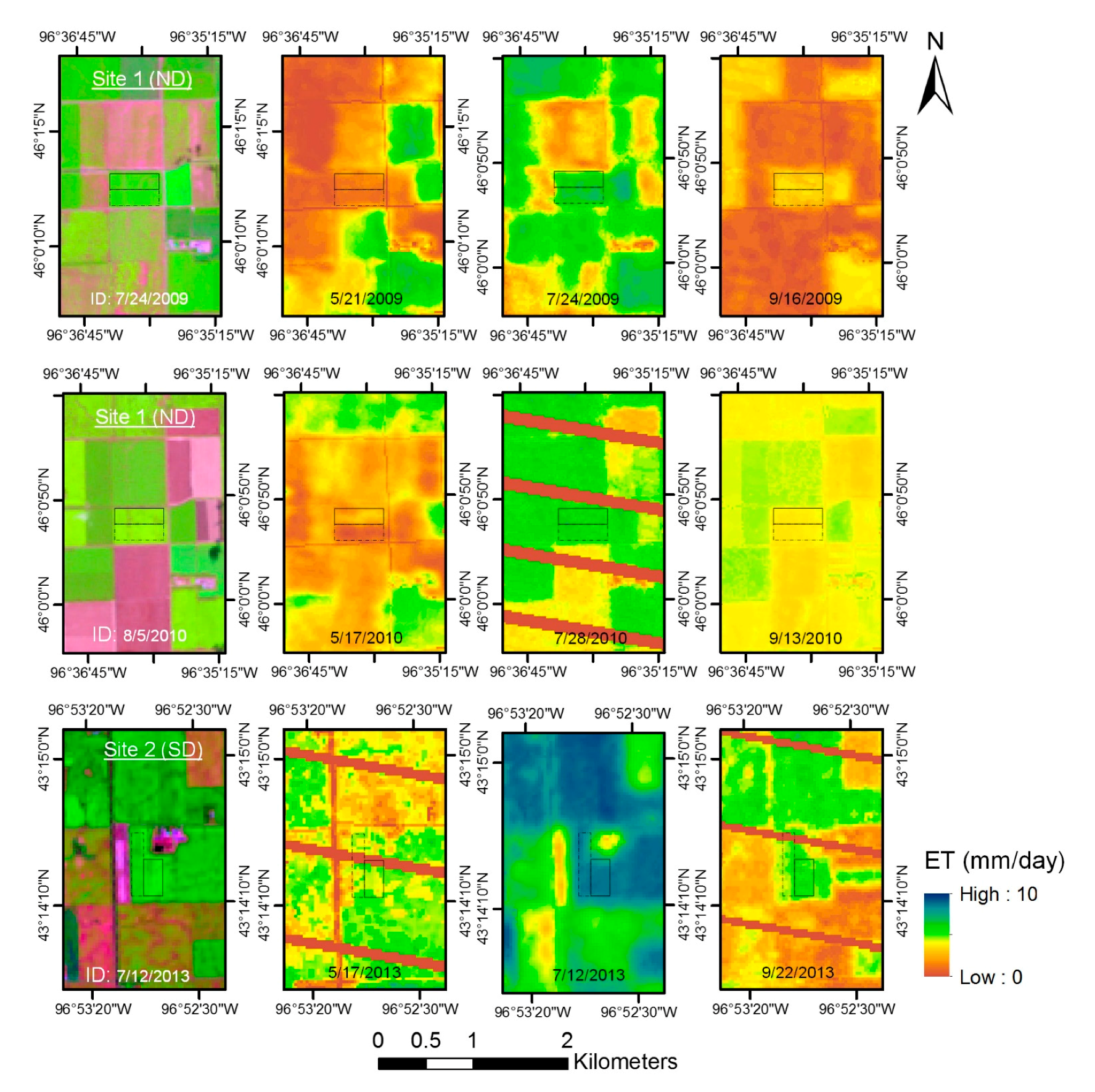
Figure 4.
Daily ET from the subsurface drained (solid rectangle) and undrained (dashed rectangle) fields for the selected Landsat image dates of May (second column), July (third column), and September (last column). The first column represents Landsat false color image (RGB: 5,4,3). ET data gaps associated with Landsat 7 images were filled by the natural neighbor interpolation method.

Figure 5.
Daily ET differences (TD–UD) at (a,b) Site 1 and (c) Site 2. The positive values indicate greater ET rates from the TD fields. Corn ET (Site 1) after October 1 to end-November, 2009 is missing due to unavailability of cloud-free Landsat image.
Figure 5.
Daily ET differences (TD–UD) at (a,b) Site 1 and (c) Site 2. The positive values indicate greater ET rates from the TD fields. Corn ET (Site 1) after October 1 to end-November, 2009 is missing due to unavailability of cloud-free Landsat image.

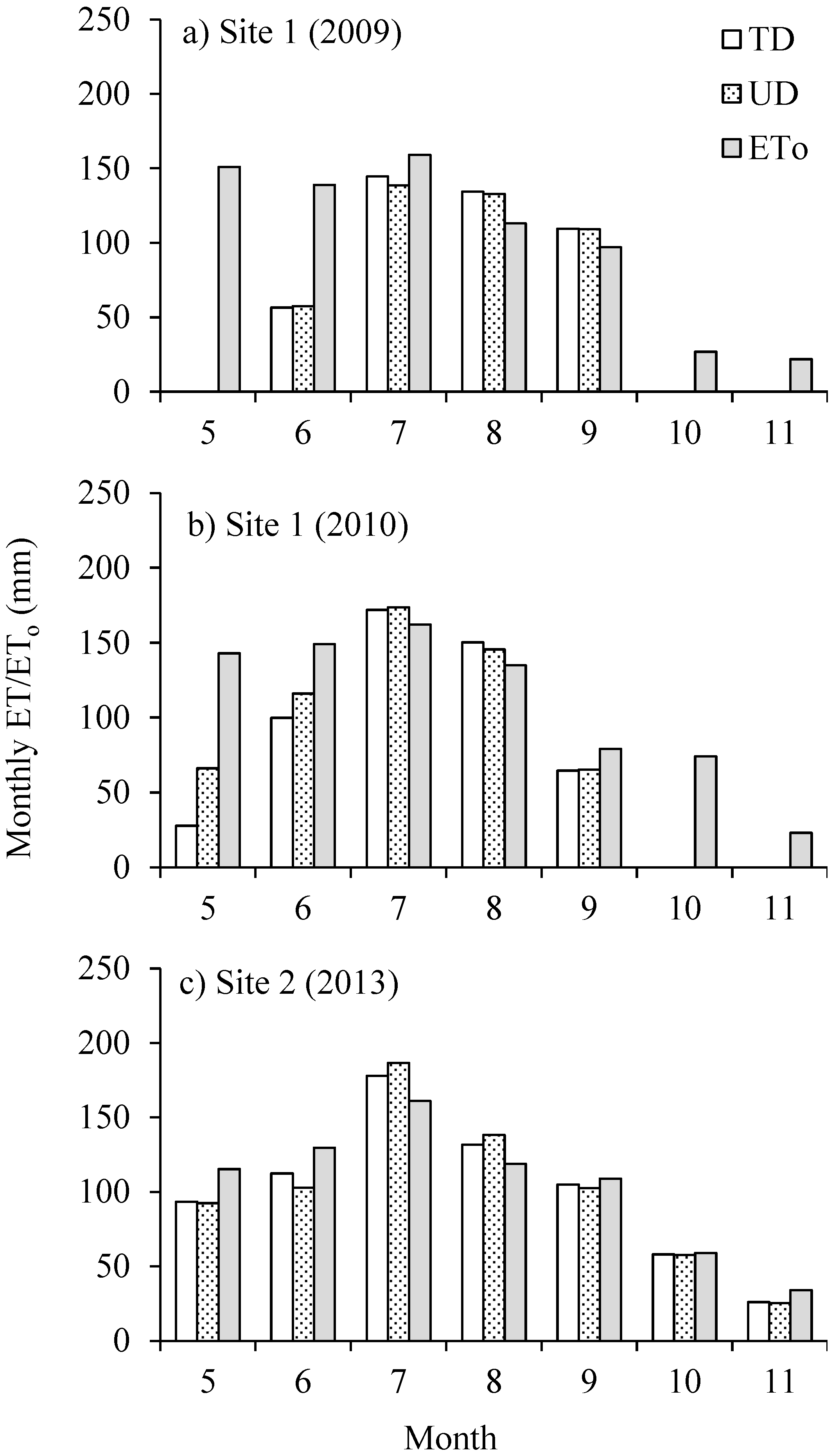
Figure 6.
Monthly ET from the subsurface drained (TD) and undrained (UD) fields estimated using METRIC, and monthly ETo estimated from weather data during the study years at (a,b) Site 1 and (c) Site 2.
Figure 6.
Monthly ET from the subsurface drained (TD) and undrained (UD) fields estimated using METRIC, and monthly ETo estimated from weather data during the study years at (a,b) Site 1 and (c) Site 2.

Table 1.
Summary of study site characteristics including drainage design information.
| Study Site | Geographic Location | Year | Crop | TD* System (Approx. Depth/Spacing) | Soil Type (Slope) |
|---|---|---|---|---|---|
| Site 1 (ND) | 46°00′45′′ N 96°35′47′′ W | 2009 and 2010 | corn (2009), soybean (2010) | 1.1 m/18.3 m | silty clay loam (≤1%) |
| Site 2 (SD) | 43°14′10′′ N 96°52′32′′ W | 2013 | corn | 1.1 m/13.7 to 30.5 m | silty clay loam (<2%) |
TD* = subsurface (tile) drainage.
Table 2.
Selected Landsat image dates with Landsat path/row and satellite information.
| Study Site | Image Date | Landsat Path/Row | Satellite |
|---|---|---|---|
| Site 1 | 21 May 2009 | 30/28 | Landsat 5 |
| 1 July 2009 | 29/28 | Landsat 5 | |
| 24 July 2009 | 30/28 | Landsat 5 | |
| 18 August 2009 | 29/28 | Landsat 5 | |
| 10 September 2009 | 30/28 | Landsat 5 | |
| 19 September 2009 | 29/28 | Landsat 5 | |
| 26 September 2009 | 30/28 | Landsat 5 | |
| 22 April 2010 | 30/28 | Landsat 5 | |
| 17 May 2010 | 29/28 | Landsat 5 | |
| 18 June2010 | 29/28 | Landsat 5 | |
| 28 July2010 | 29/28 | Landsat 7 | |
| 5 August 2010 | 29/28 | Landsat 5 | |
| 28 August 2010 | 30/28 | Landsat 5 | |
| 13 September 2010 | 30/28 | Landsat 5 | |
| 8 October 2010 | 29/28 | Landsat 5 | |
| Site 2 | 17 May 2013 | 29/30 | Landsat 7 |
| 18 June 2013 | 29/30 | Landsat 7 | |
| 12 July2013 | 29/30 | Landsat 8 | |
| 29 August 2013 | 29/30 | Landsat 8 | |
| 22 September 2013 | 29/30 | Landsat 7 | |
| 17 November 2013 | 29/30 | Landsat 8 |
Table 3.
ET from the subsurface drained (TD) and undrained (UD) field, rainfall, and reference ET for the June–September period.
Table 3.
ET from the subsurface drained (TD) and undrained (UD) field, rainfall, and reference ET for the June–September period.
| Study Year | Month | ET (mm) | Rain (mm) | ETo (mm) | |
|---|---|---|---|---|---|
| TD | UD | ||||
| 2009 (corn) | JJ | 201 | 196 | 115 | 298 |
| JA | 279 | 272 | 109 | 272 | |
| AS | 244 | 242 | 138 | 210 | |
| 2010 (soybean) | JJ | 272 | 290 | 134 | 311 |
| JA | 322 | 319 | 135 | 297 | |
| AS | 215 | 211 | 216 | 214 | |
| 2013 (corn) | JJ | 290 | 289 | 106 | 290 |
| JA | 309 | 325 | 108 | 280 | |
| AS | 236 | 240 | 115 | 227 | |
JJ = June–July; JA = July–August; AS = August–September.
© 2017 by the authors. Licensee MDPI, Basel, Switzerland. This article is an open access article distributed under the terms and conditions of the Creative Commons Attribution (CC BY) license (http://creativecommons.org/licenses/by/4.0/).
Share and Cite
MDPI and ACS Style
Khand, K.; Kjaersgaard, J.; Hay, C.; Jia, X. Estimating Impacts of Agricultural Subsurface Drainage on Evapotranspiration Using the Landsat Imagery-Based METRIC Model. Hydrology 2017, 4, 49. https://doi.org/10.3390/hydrology4040049
AMA Style
Khand K, Kjaersgaard J, Hay C, Jia X. Estimating Impacts of Agricultural Subsurface Drainage on Evapotranspiration Using the Landsat Imagery-Based METRIC Model. Hydrology. 2017; 4(4):49. https://doi.org/10.3390/hydrology4040049
Chicago/Turabian StyleKhand, Kul, Jeppe Kjaersgaard, Christopher Hay, and Xinhua Jia. 2017. "Estimating Impacts of Agricultural Subsurface Drainage on Evapotranspiration Using the Landsat Imagery-Based METRIC Model" Hydrology 4, no. 4: 49. https://doi.org/10.3390/hydrology4040049
Note that from the first issue of 2016, this journal uses article numbers instead of page numbers. See further details here.