On Rigorous Drought Assessment Using Daily Time Scale: Non-Stationary Frequency Analyses, Revisited Concepts, and a New Method to Yield Non-Parametric Indices


Abstract
1. Introduction
2. Methods
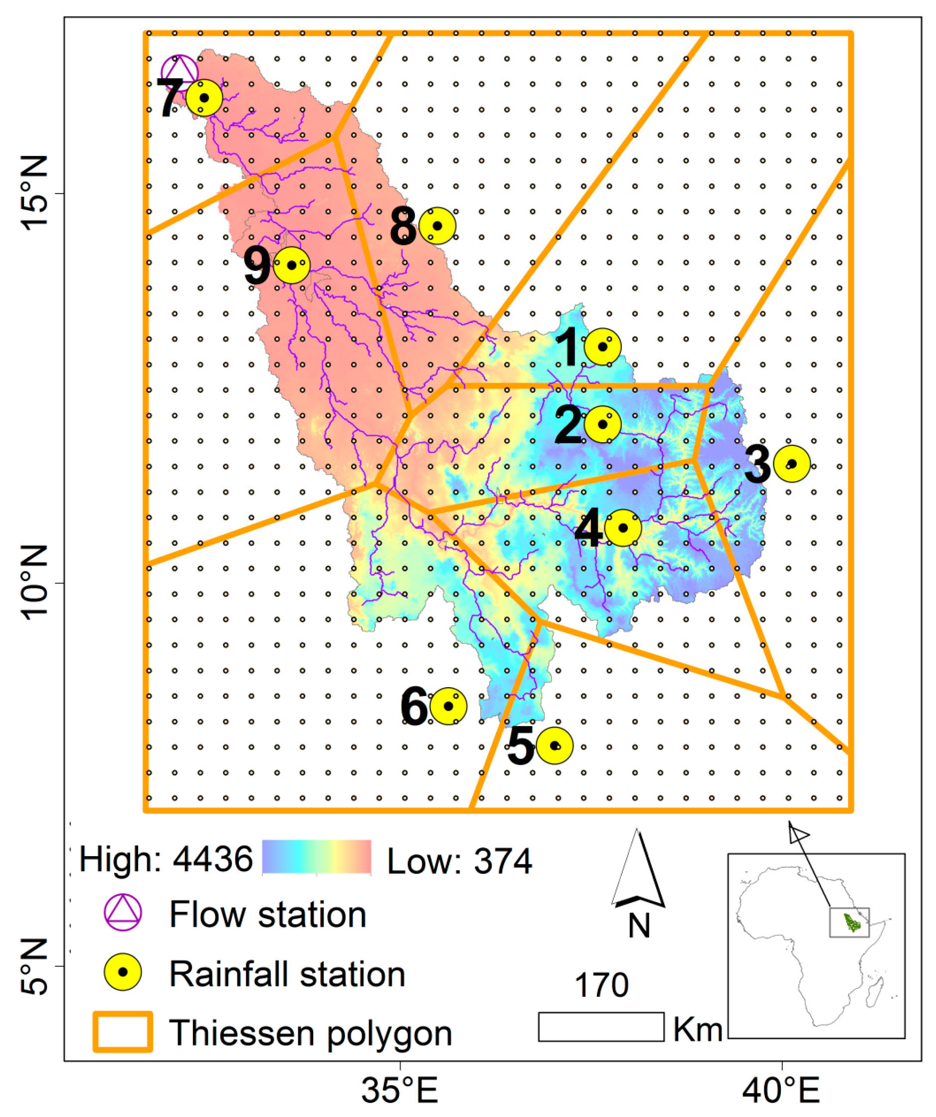
2.1. Data for the Case Study
2.2. Stationarity versus Non-Stationarity
2.2.1. Pre-Requisites for Frequency Analysis
Data Transformation
Independence of the Extreme Events
- (i)
- the time in between the two events should not be less than the stipulated value;
- (ii)
- the extracted event should not be less than the specified threshold; and
- (iii)
- the independency ratio should not be greater than a stipulated value.
Significance of Trend in the Data
2.2.2. Frequency Analyses of Stationary Extremes
2.2.3. Frequency Analyses of Non-Stationary Extremes
Method 1: The use of significance of quantiles
can be computed using where RT is obtained using Equation (17) or (18) depending on the shape parameter γ.Method 2: The use of statistical simulation of extreme events
- (1)
- Obtain the plot of POTs versus the RTOs and compute the intercept of the linear trend line.
- (2)
- Detrend the POTs to obtain Qi = POTi − (m × RTOi + intercept) for i = 1, 2, ..., n′. Obtain Qmin i.e., the absolute value of the minimum residual time series Qi using Qmin = |min(Qi)|.
- (3)
- Investigate which correlation model the extreme events follow. The persistence model can be used for generating the synthetic extreme events. Assuming that the remaining persistence in the POTs following the application of the independence criteria for extracting the extreme events is of the lag-1 autoregressive AR(1) process, compute the AR(1) serial correlation coefficient r1 of the detrended time series Qi using Equation (10). The AR(1) was assumed for illustration purpose. Persistence may be of the forms characterized by the fractional Gaussian noise, fractionally integrated autoregressive moving average, autoregressive integrated moving average, discrete fractional Brownian motion, fractionally differenced process, etc.
- (4)
- Obtain W and N such that N = βn′ and W (in year) = βw, where β determines the length of the synthetic events, while w and n′ are as defined shortly before. For instance, in this paper, β was set to 2 as a precaution to minimize the possible introduction of uncertainty in the extreme value analysis due to finite sample size.
- (5)
- Let θ1 denote the RTO of the first POT event. Generate the serial number Φ for the synthetic time series using Φi = θ1 + Δ × (i − 1) for i = 1, 2, ..., N, where Δ = (365.25 × W)/N. The value of Φ should be rounded to a whole number.Obtain two trend lines based on the values of Φ. Using the trend slope m from Equation (1) and the intercept computed from Step (1), obtain the first trend line L1 using L1,i = (m × Φi + intercept) where i = 1, 2, ..., N. Using the Qmin from Step (2), obtain the second line L2,i = L1,i − Qmin. The second line L2 is to ensure that the synthetic events do not go below the threshold used in the independence criteria for extraction of the POTs from the original or full time series.
- (6)
- Generate large number, say, Nsim, of synthetic time series using Equation (19) based on the relevant persistence model identified in Step (3). In this case, for illustration, based on first-order (Markov) AR stochastic process assumed in Step (3), the synthetic extreme events were generated using:where E(G) is the mean of Gi (i.e., the POT events), G0 denotes the first POT event, εi is the white-noise process with mean με = 0 and standard deviation σε. Based on the standard deviation SD of the POT events, σε = SD × (1 − )0.5 and r1 is as defined in Step (3).Superimpose, for i = 1, 2, ..., N, the linear trend onto the time series using G1,i = Gi + L1,i − E(G). Eventually, for i = 1, 2, ..., N, the final synthetic events Gsys = G1,i if G1,i ≥ L2,i or Gsys = (G1,i + L2,i + Qmin) when G1,i < L2,i.
- (7)
- The simulation procedure will yield synthetic extreme events in the form of a matrix of N rows and Nsim columns. For each row, rank, in descending order, the Nsim synthetic events. Construct the upper and lower limits of the (100-αs)% confidence interval on the synthetic event of each row using (0.005 × αs% × Nsim)th and ({1 − [0.005 × αs%]} × Nsim)th ranked values, respectively. Similarly, compute the mean of the Nsim values in each row. Rank the computed mean values, as well as the (100-αs)% confidence interval limits from the highest to the lowest. Finally, compute the return period T (in years) of the synthetic values as the ratio of W (in years) to the rank j of the synthetic events (ordered such that j = 1 is for the highest ranking value).
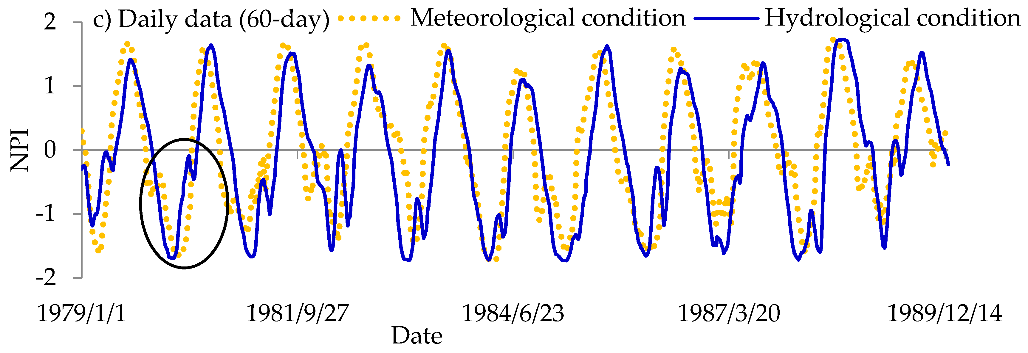
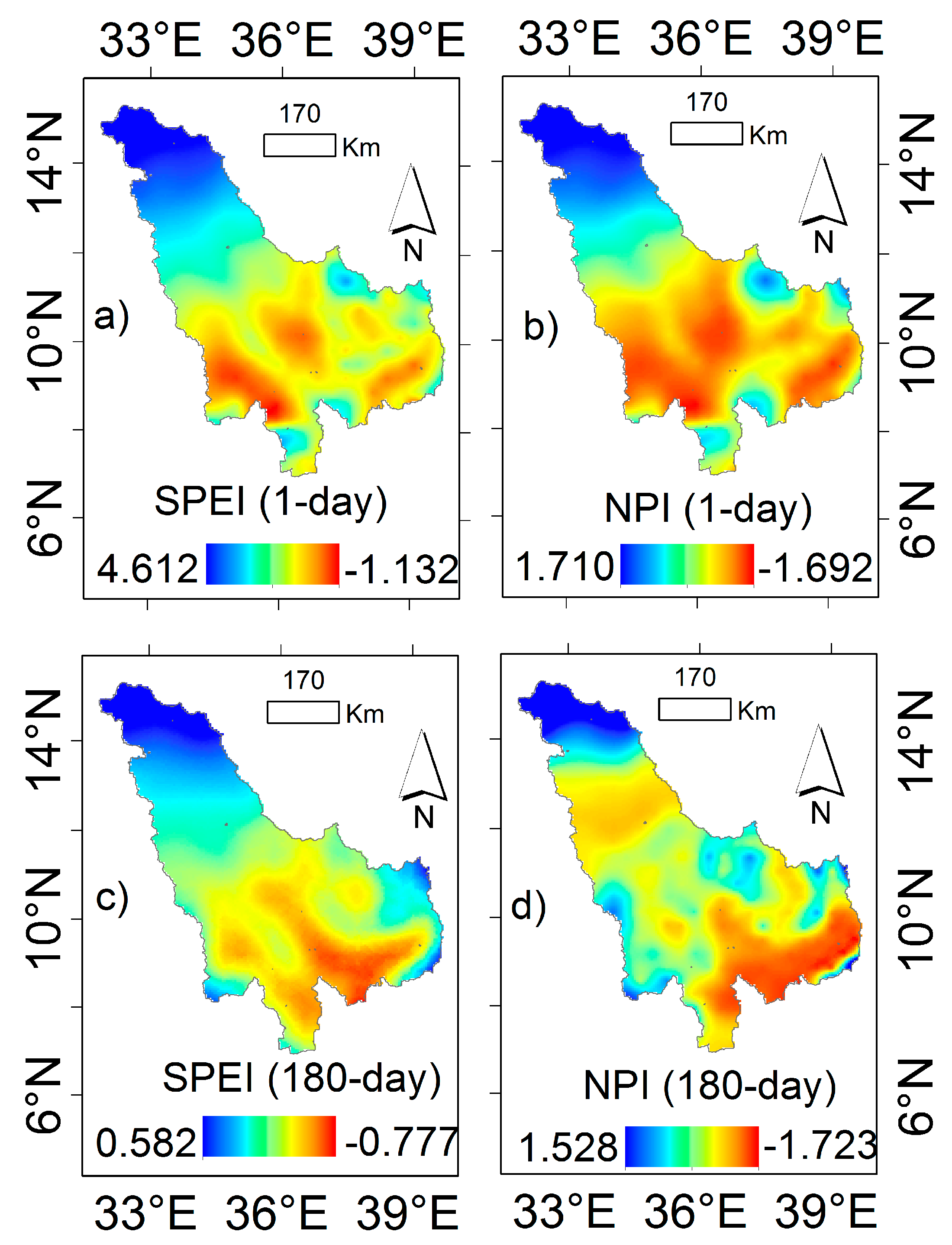
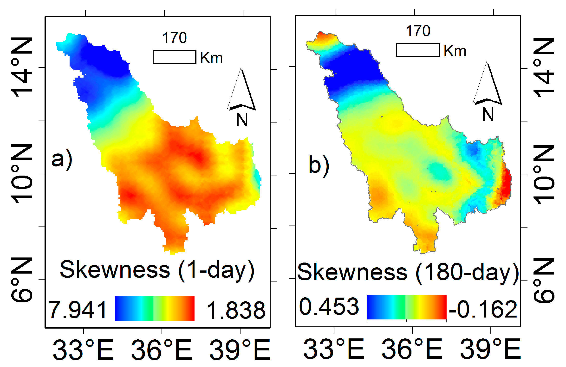
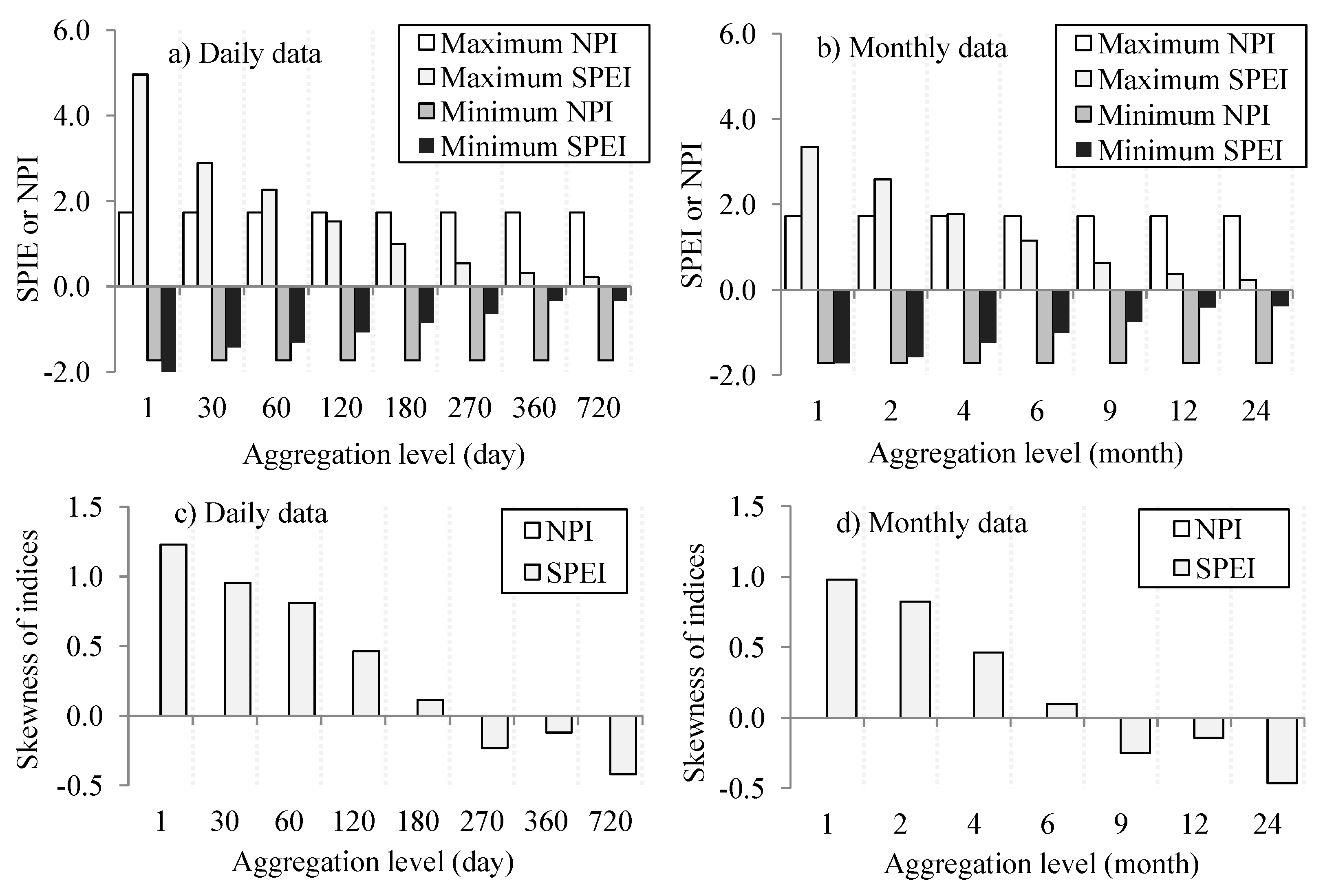
2.2.4. Non-Parametric Indices (NPIs) for Drought Assessment
3. Results and Discussion
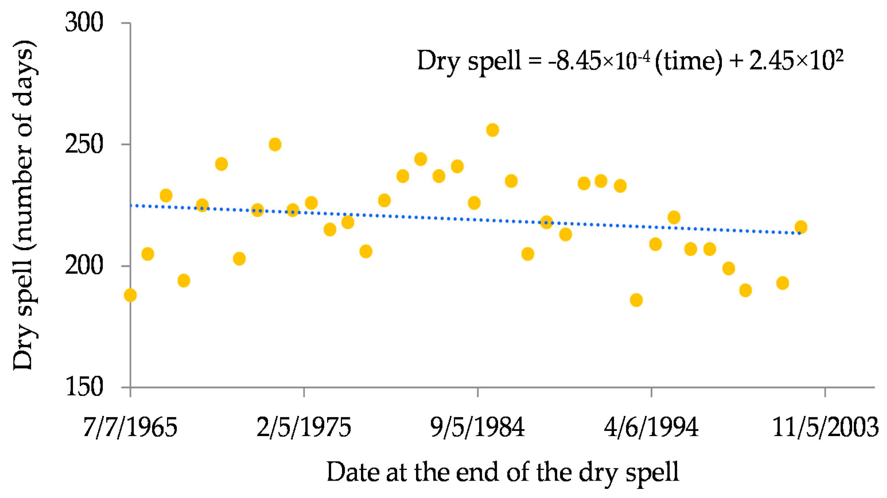
3.1. Statistical Trend Analyses
3.2. Frequency Analyses of Stationary Extremes
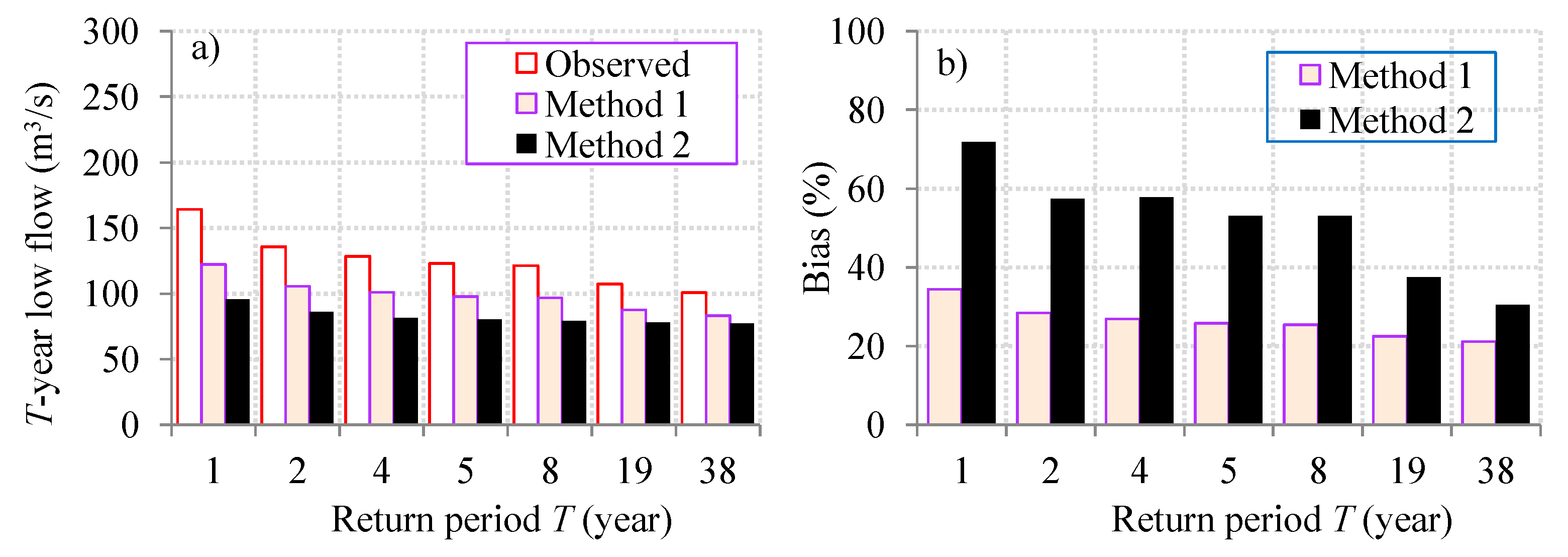
3.3. Frequency Analyses of Non-Stationary Extremes
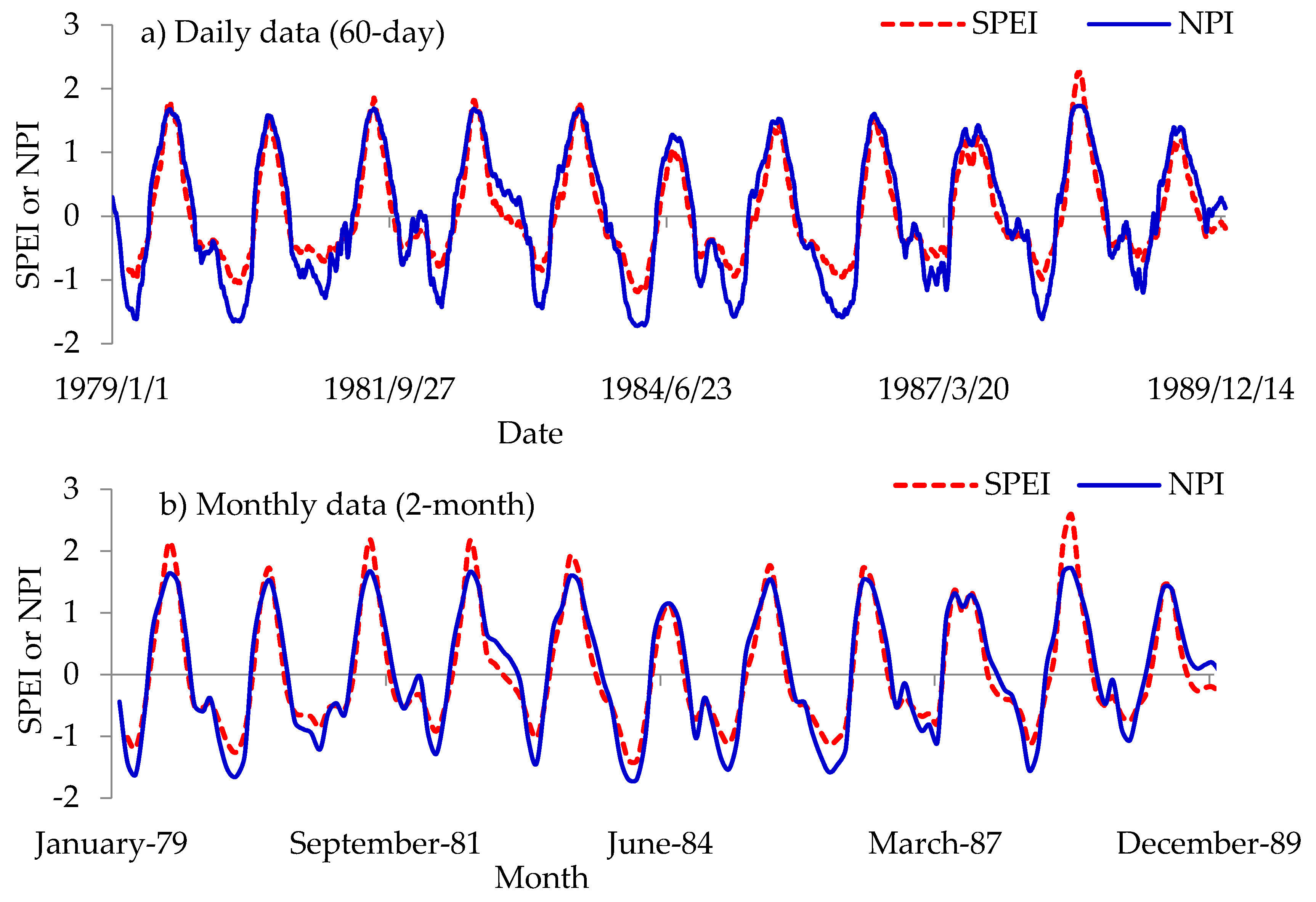
3.4. Non-Parametric Indices (NPIs) for Drought Assessment
4. Conclusions
Acknowledgments
Conflicts of Interest
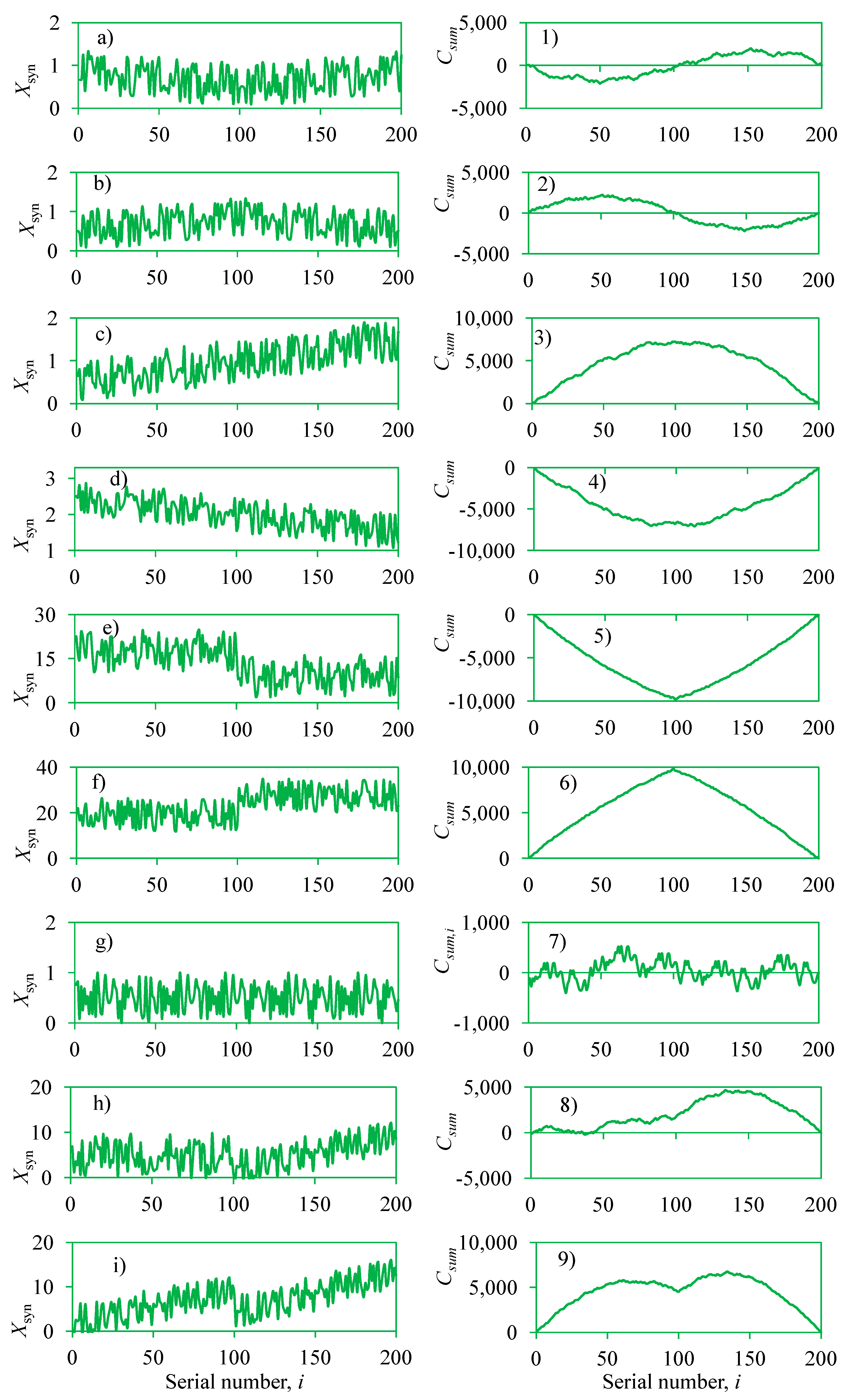
Appendix A. Performance of the CSD Trend Statistic Variance Correction
Appendix B. Graphical Diagnoses of Changes Based on CSD Trend Test
Appendix C. Revisiting Concepts on Drought Assessment through Shift from Coarse to Fine Temporal Scale
C.1. Introduction
C.2. Definitions of Key Drought Terms Based on Daily Time Scale
C.2.1. Threshold
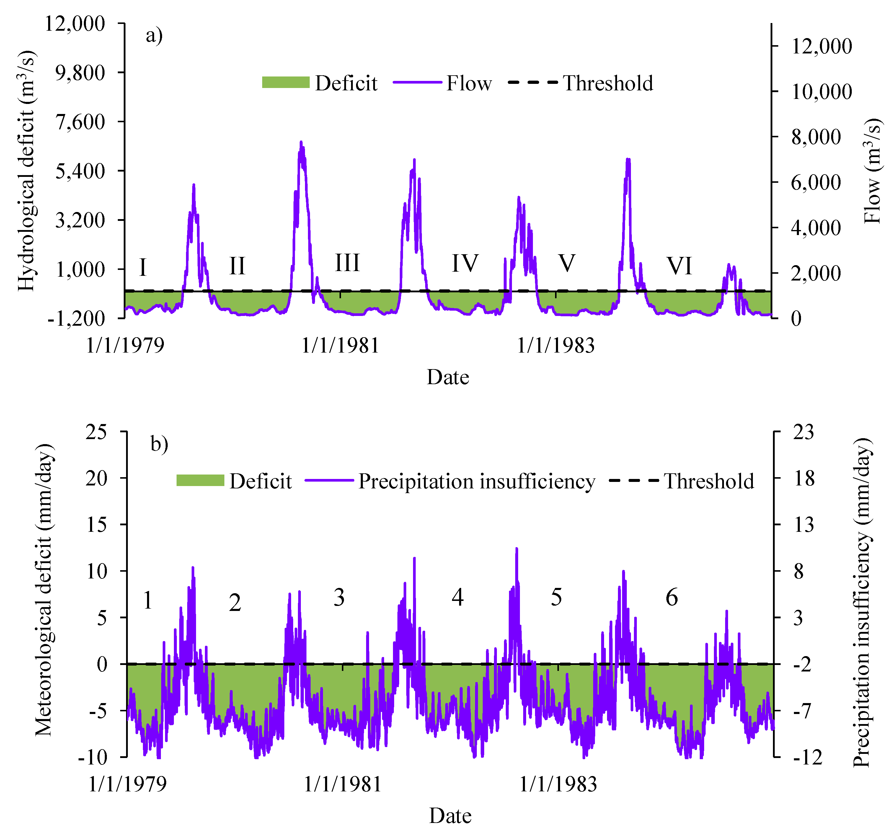
C.2.2. Deficit, Deficit Period, Drought Intensity and Extremity
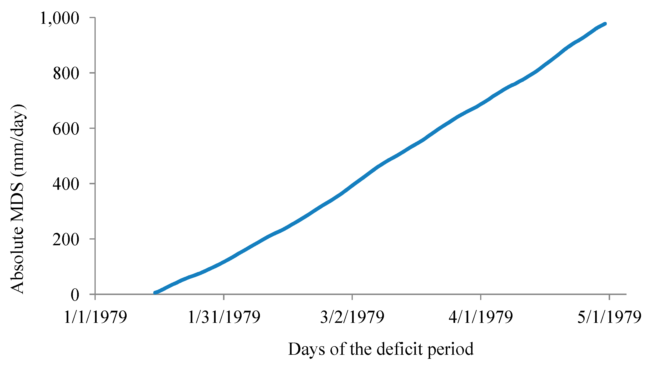
C.2.3. Deficit Sum versus Days of Deficit Period
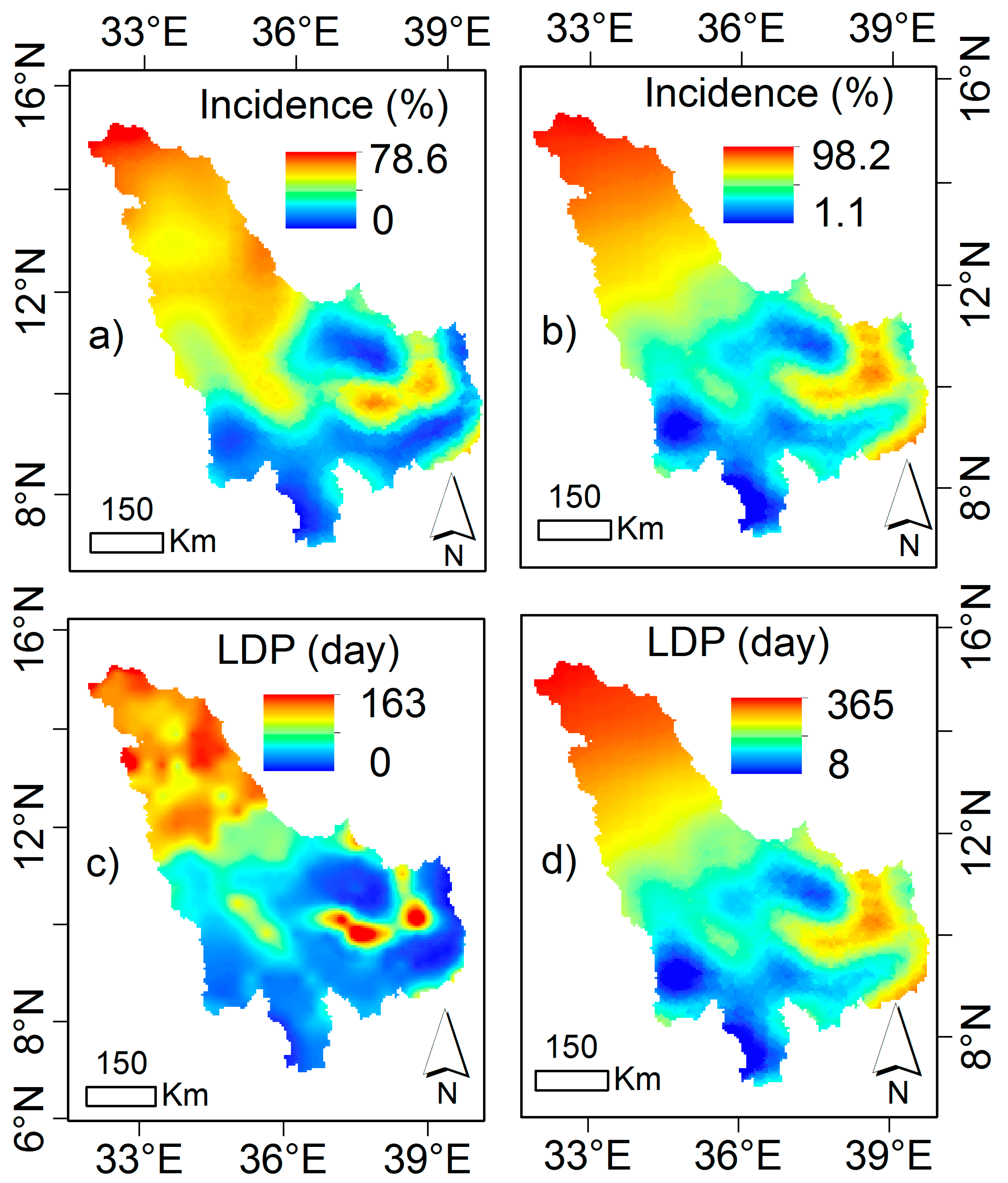
C.2.4. Drought Quantile and Incidence
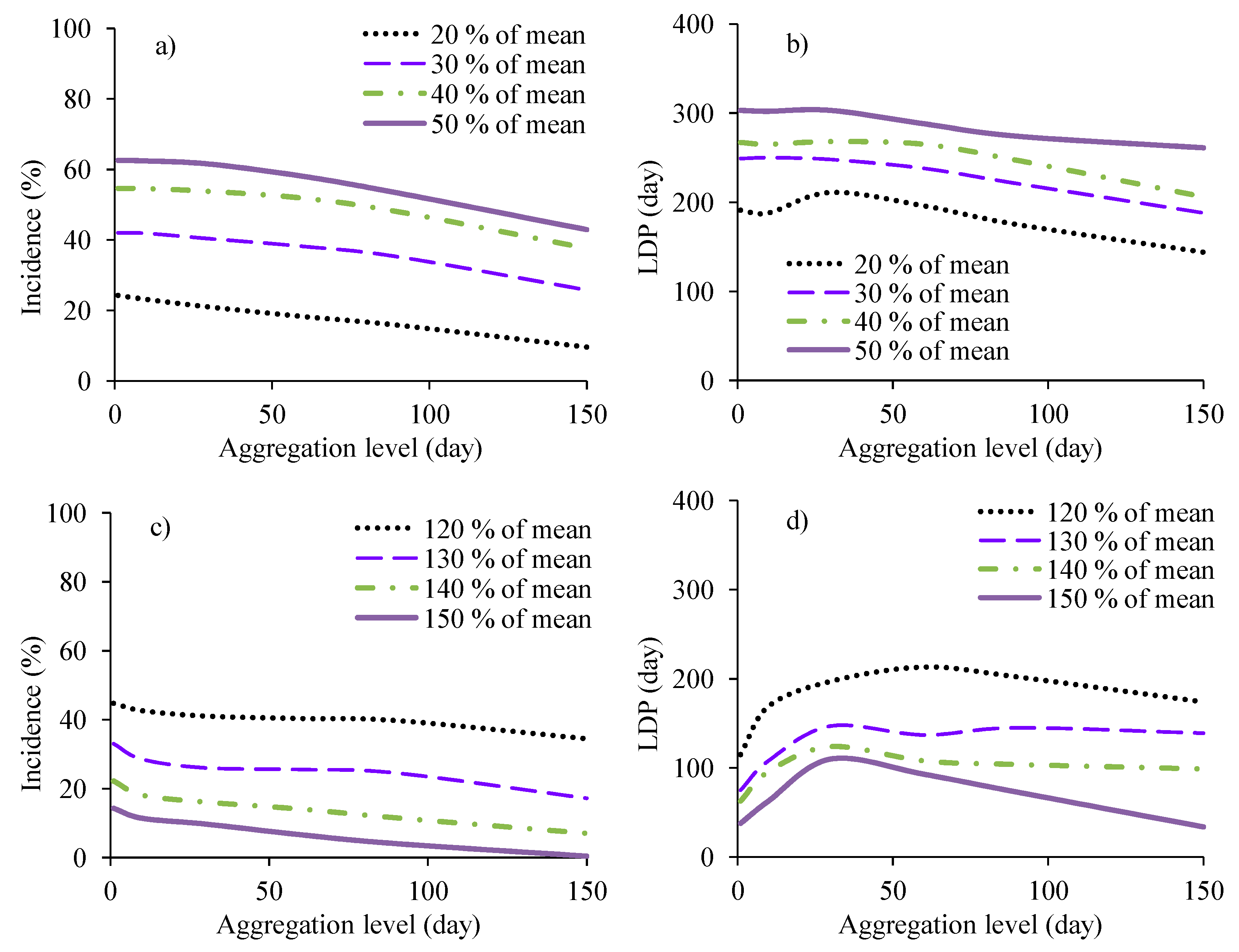
C.2.5. Relationships between Deficit or Incidence with Threshold and Duration
- (1)
- Select aggregation levels (Aagg). For illustration in this paper, the values of Aagg were set to 1, 7, 15, 30, 60, 90 and 150 days. In reality, the range of Aagg to be selected should be relevant for the intended application. Next, pass an overlapping moving averaging window of length equal to each Aagg using Equations (20)–(24).
- (2)
- Select thresholds for determining the deficit period. In this study, 20, 30, 40 and 50% of the long-term mean of daily river flow, and 120, 130, 140 and 150% of the long-term mean of daily precipitation insufficiency were selected.
- (3)
- For each threshold, compute the historical LDP and incidence based on the aj’s from each value of Aagg from Step 1. The last step is the compilation of the LDP and incidence for the various thresholds and values of Aagg to constitute LDP-DT and IDT relationships respectively.
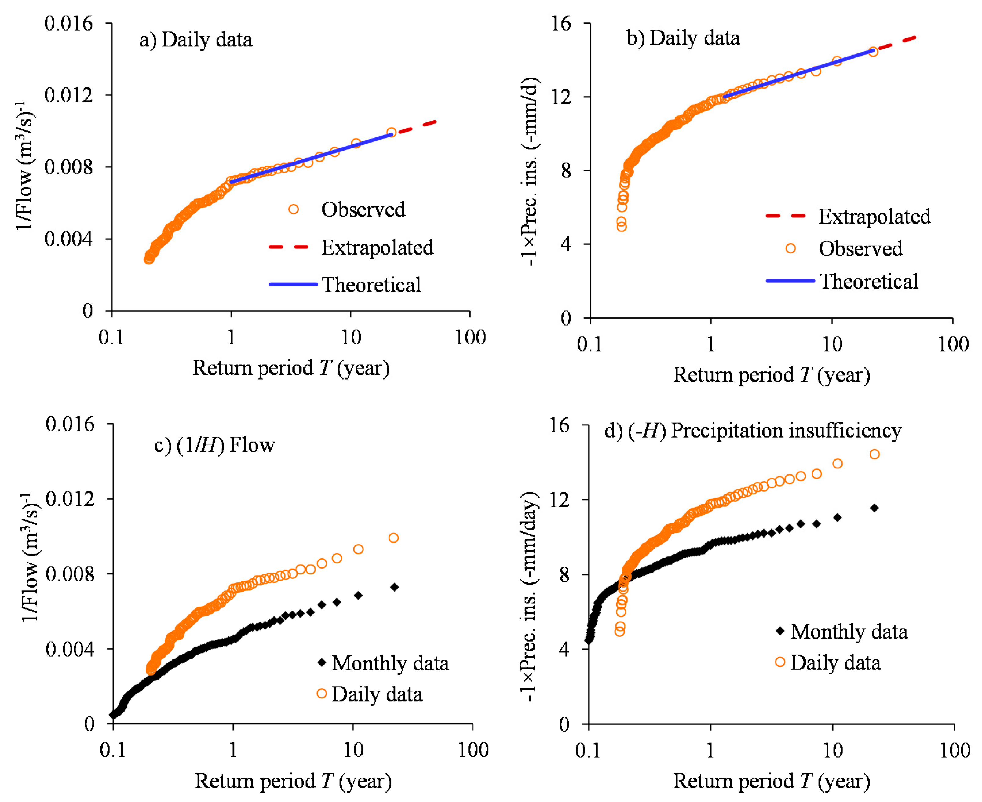
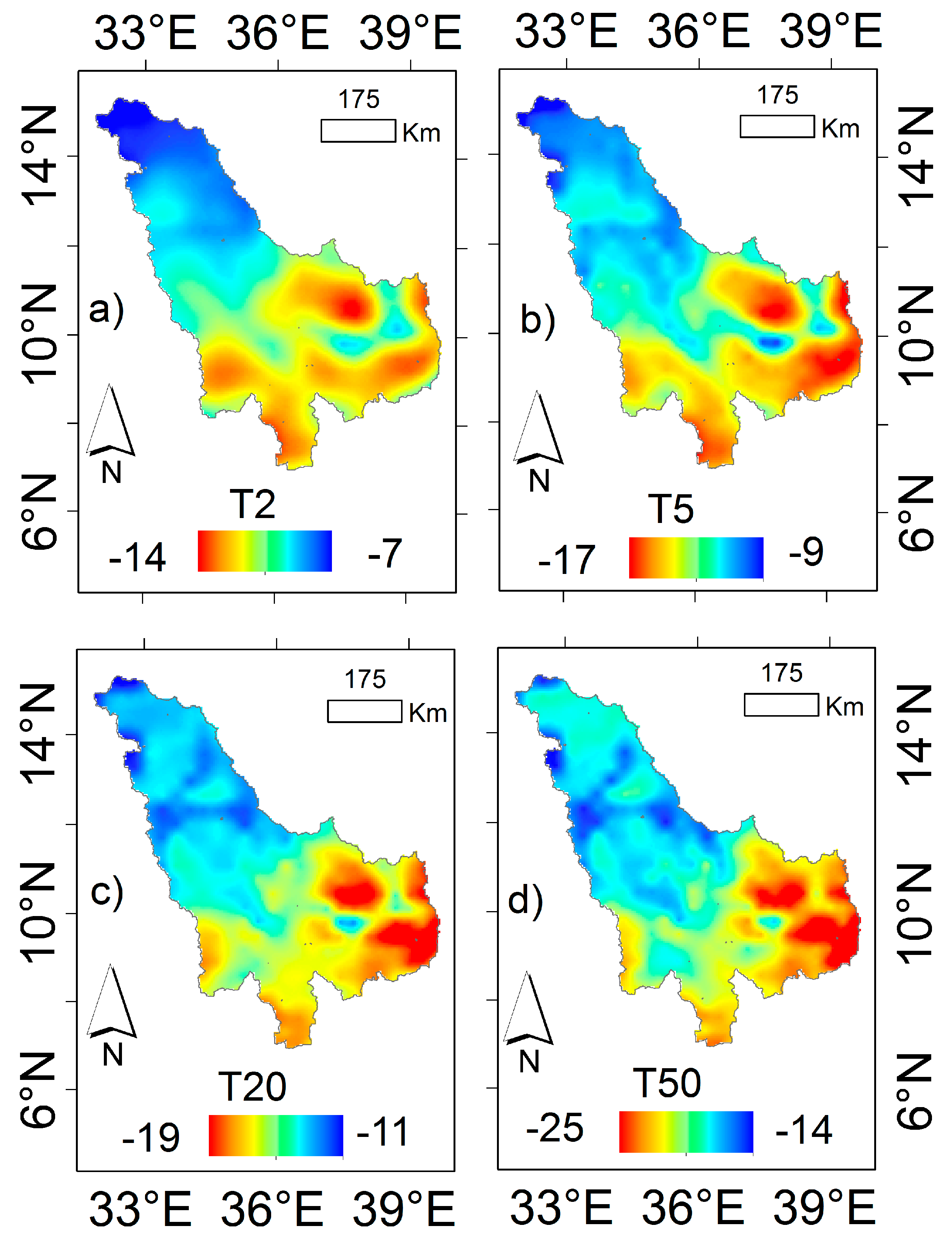
C.2.6. Amplitude–Duration–Frequency Relationships
- (1)
- Transform river flow (H) and precipitation insufficiency (H) using (1/H) and (-H), respectively.
- (2)
- Select various values of Aagg with the range relevant for the intended application.
- (3)
- For each of the Aagg values, perform:
- (a)
- temporal aggregation of the series using Equation (20);
- (b)
- extraction of the POT events using the independence criteria from Section 2.2.1; since aggregation may bring about auto-correlation, the specifications of these criteria can be in a relaxed or stringent way based on whether small or large values of Aagg have been used to smoothen the data;
- (c)
- selection of various T’s relevant for the intended application; and
- (d)
- derivation, for the corresponding T’s, the return levels assuming H is from stationary or non-stationary process using the details of methodology presented in Section 2.2.2 and Section 2.2.3.
- (4)
- Compile back-transformed quantiles for the various T’s and Aagg values.
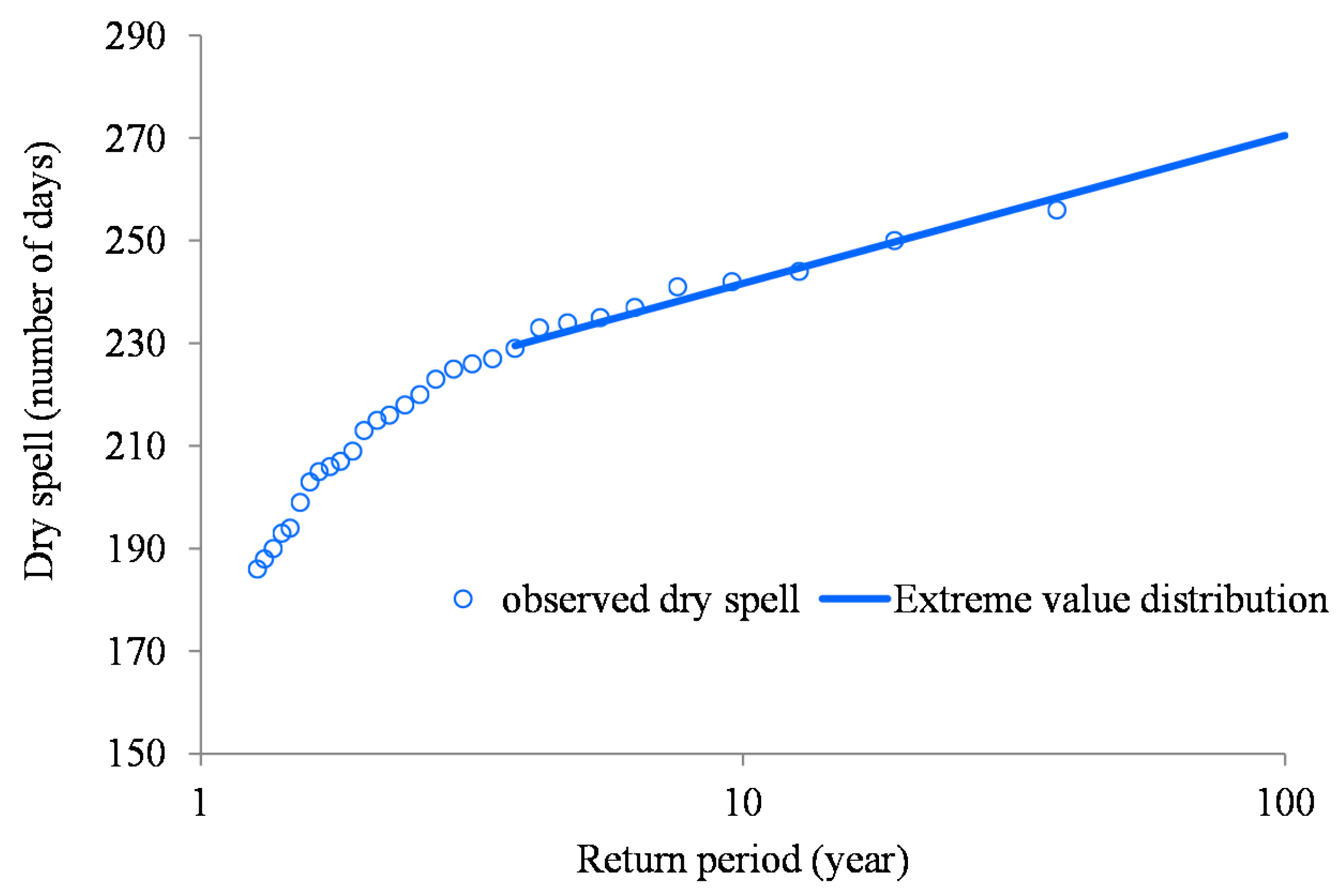
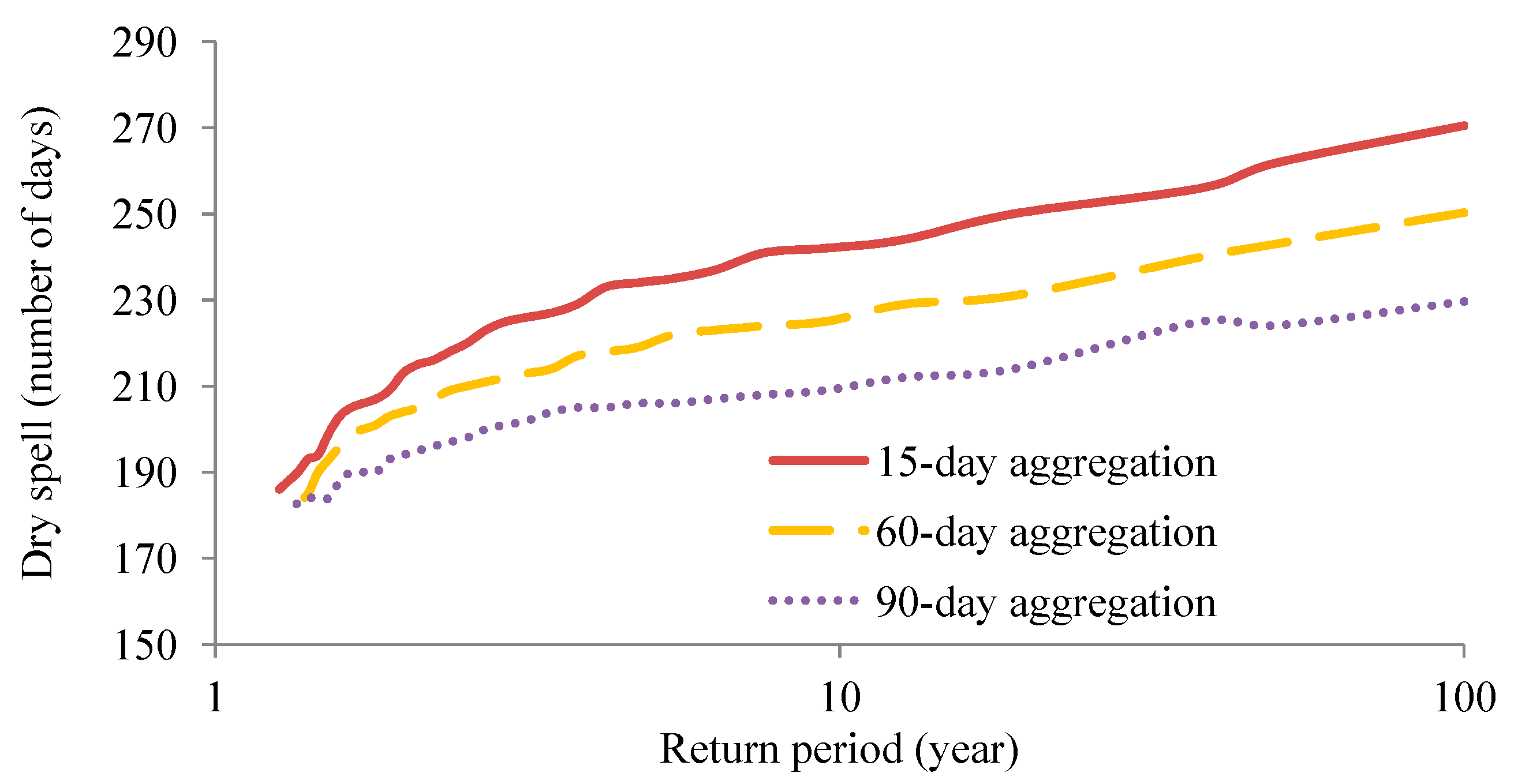
C.2.7. Relationship between Dry Spell or Deficit Period, Duration and Frequency
- (1)
- Values of Aagg were set to 15, 60 and 90 days and Equation (20) was applied to the time series.
- (2)
- For each Aagg, hydrological dry spells or deficit periods were independent (or nearly so). Expressly, daily flow threshold was set to 800 m3/s, and the minimum number of days to characterize a hydrological dry spell was set to 175 days.
- (3)
- For each Aagg, empirical T was computed for the independent dry spells. Theoretical dry spell DT for a given T was estimated using DT = η × {log(T) − log(Th)} + Dh where Dh is the threshold dry spell, Th is the return period of Dh, and η is the slope of the line fitted above the threshold. To estimate η, log-transformed empirical T is plotted against the dry spell. The slope of the logarithmic line fitted to the events above the Dh gives the η estimate.
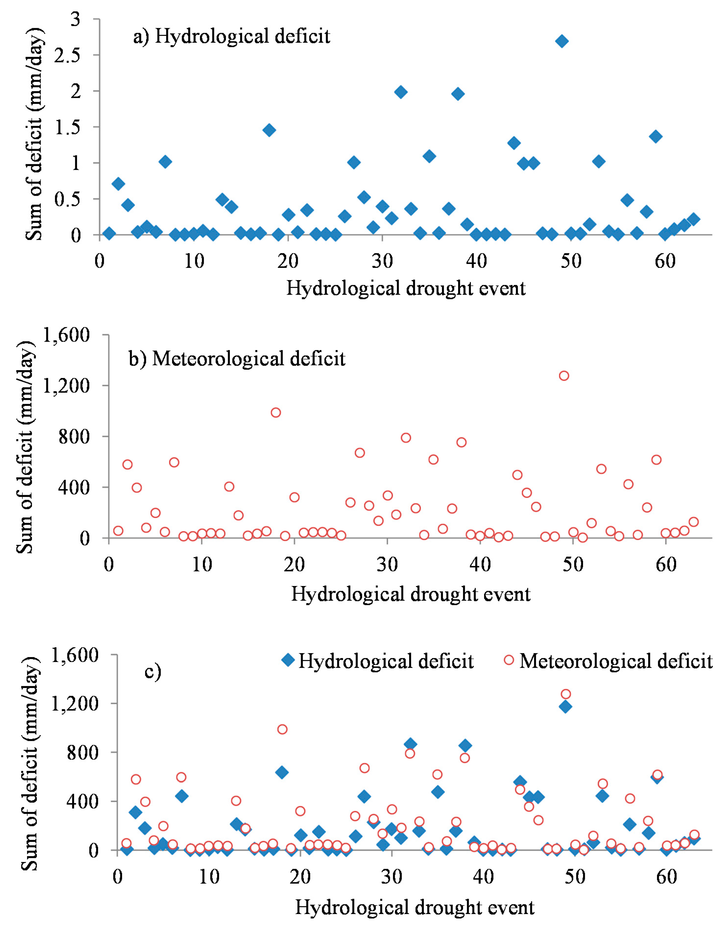
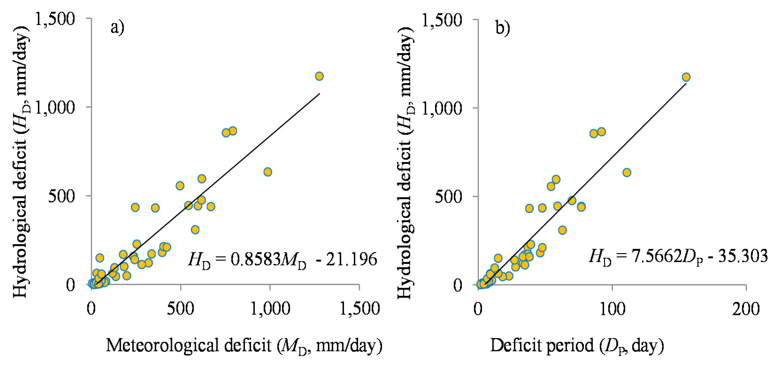
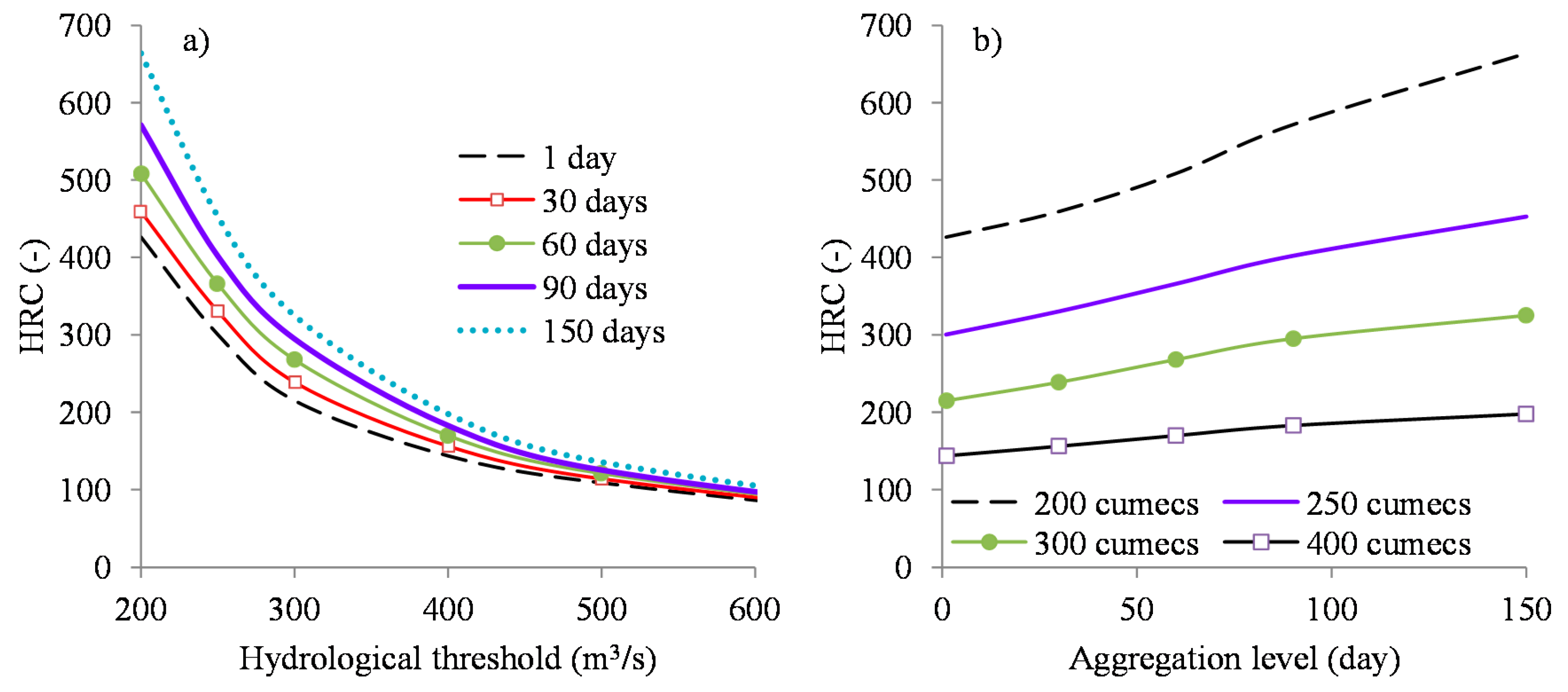
C.2.8. Hydrological Response to Meteorological Drought
- (1)
- Set the relevant hydrological or flow thresholds. In this study, for illustration, daily flow thresholds were set to 200, 500, 750 m3/s, etc.
- (2)
- Determine the hydrological deficit periods.
- (3)
- For each deficit period or drought event, obtain the absolute sum of the hydrological deficits (m3/s). Multiply each daily hydrological deficit by (86.4/CA) where CA is the catchment area in km2. This converts all the obtained deficits from m3/s to mm/day to match the unit of the precipitation insufficiency.
- (4)
- For each corresponding daily hydrological deficit period, obtain the absolute sum of the precipitation insufficiency (mm/day).
- (5)
- By trial and error, look for a constant (hereinafter taken as the HRC) by which when all the sums of the hydrological deficits are multiplied, the difference between the meteorological and hydrological deficits becomes minimal. This can be done by mean squared error minimization technique. Expectedly, the scatter plots of the hydrological versus meteorological deficits should exhibit a linear relationship. For an ideal system, the line passes through the origin and has a slope equal to 1.
- (6)
- Repeat Steps 2 to 5 for various Aagg values. Finally, compile the HRCs from the various Aagg values and thresholds to comprise the HRC–DT relationships.
C.3. Applications of Daily Time Scale for Drought Analyses
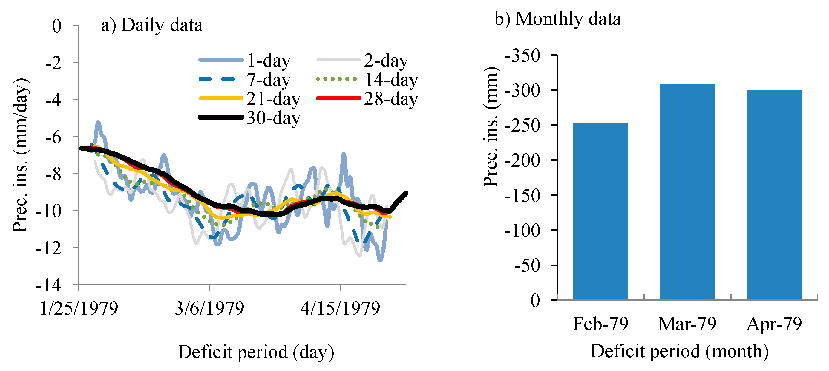
C.3.1. Threshold and Deficits
C.3.2. Deficit Sum versus Days of Deficit Period
C.3.3. Drought Quantile and Incidence
C.3.4. Relationships between Deficit or Incidence with Threshold and Duration
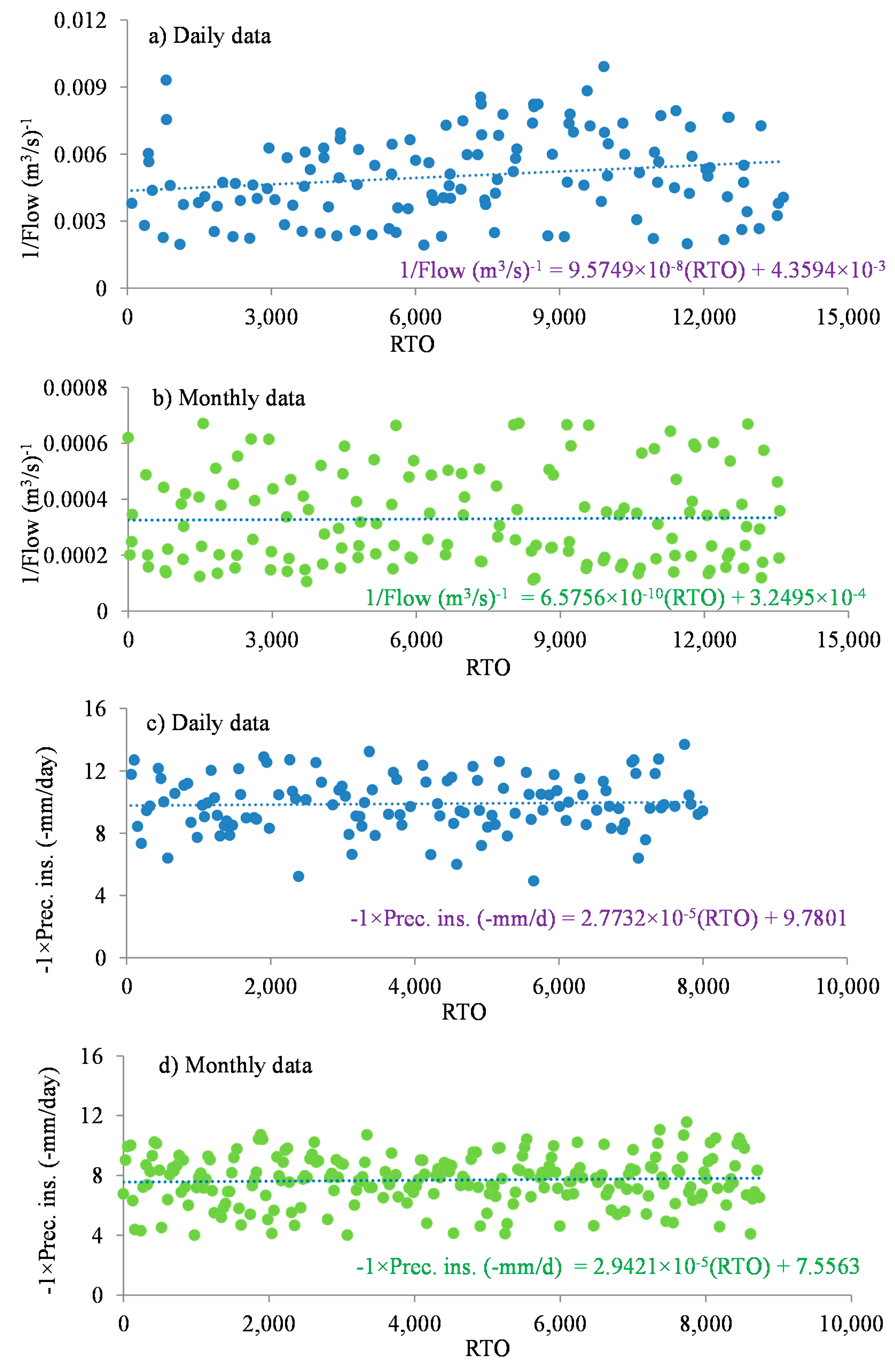
C.3.5. Amplitude–Duration–Frequency Relationships
C.3.6. Relationship between Dry Spell or Deficit Period, Duration and Frequency
C.3.7. Hydrological Response to Meteorological Drought
References
- Wilhite, D.A.; Glantz, M.H. Understanding: The drought phenomenon: The role of definitions. Water Int. 1985, 10, 111–120. [Google Scholar] [CrossRef]
- Kogan, F.N. Global drought watch from space. Bull. Am. Meteorol. Soc. 1997, 78, 621–636. [Google Scholar] [CrossRef]
- Wilhite, D.A.; Buchanan-Smith, M. Drought as hazard: Understanding the natural and social context. In Drought and Water Crises: Science, Technology, and Management Issues; Wilhite, D.A., Ed.; Taylor and Francis: Boca Raton, FL, USA, 2005; pp. 3–29. [Google Scholar]
- Palmer, W.C. Keeping track of crop moisture conditions, nationwide. The new crop moisture index. Weatherwise 1968, 21, 156–161. [Google Scholar] [CrossRef]
- McKee, T.; Doesken, N.; Kleist, J. The relationship of drought frequency and duration to time scales. In Proceedings of the 8th Conference of Applied Climatology, Anaheim, CA, USA, 17–22 January 1993; pp. 179–184. [Google Scholar]
- Bloomfield, J.P.; Marchant, B.P. Analysis of groundwater drought building on the standardised precipitation index approach. Hydrol. Earth Syst. Sci. 2013, 17, 4769–4787. [Google Scholar] [CrossRef]
- Vicente-Serrano, S.M.; Beguería, S.; López-Moreno, J.I. A multiscalar drought index sensitive to global warming: The standardized precipitation evapotranspiration index. J. Clim. 2010, 23, 1696–1718. [Google Scholar] [CrossRef]
- Palmer, W.C. Meteorological Drought; Research Paper No 45; US Weather Bureau: Washington, DC, USA, 1965.
- Abramowitz, M.; Stegun, I.A. Handbook of Mathematical Functions with Formulas, Graphs, and Mathematical Table; Courier Dover Publications: Mineola, NY, USA, 1965. [Google Scholar]
- Stagge, J.A.; Tallaksen, L.M.; Gudmundsson, L.; Van Loon, A.F.; Stahle, K. Candidate distributions for climatological drought indices (SPI and SPEI). Int. J. Climatol. 2015, 35, 4027–4040. [Google Scholar] [CrossRef]
- Stagge, J.A.; Tallaksen, L.M.; Gudmundsson, L.; Van Loon, A.F.; Stahle, K. Short communication response to comment on Candidate Distributions for Climatological Drought Indices (SPI and SPEI). Int. J. Climatol. 2016, 36, 2132–2138. [Google Scholar] [CrossRef]
- Vicente-Serrano, S.M.; Beguería, S. Short communication comment on “candidate distributions for climatological drought indices (SPI and SPEI)” by James H. Stagge et al. Int. J. Climatol. 2016, 36, 2120–2131. [Google Scholar] [CrossRef]
- Sawada, Y.; Koike, T.; Jaranilla-Sanchez, P.A. Modeling hydrologic and ecologic responses using a new eco-hydrological model for identification of droughts. Water Resour. Res. 2014, 50, 6214–6235. [Google Scholar] [CrossRef]
- Cancelliere, A. Non stationary analysis of extreme events. Water Resour. Manag. 2017, 31, 3097–3110. [Google Scholar] [CrossRef]
- Wang, Y.; Li, L.; Feng, P.; Hu, R. A time-dependent drought index for non-stationary precipitation series. Water Resour. Manag. 2015, 29, 5631–5647. [Google Scholar] [CrossRef]
- Mu, Q.; Zhao, M.; Running, S.W. Improvements to a MODIS global terrestrial evapotranspiration algorithm. Remote Sens. Environ. 2011, 115, 1781–1800. [Google Scholar] [CrossRef]
- Anderson, M.C.; Hain, C.; Otkin, J.; Zhan, X.; Mo, K.; Svoboda, M.; Wardlow, B.; Pimstein, A. An Intercomparison of drought indicators based on thermal remote sensing and NLDAS-2 simulations with U.S. drought monitor classifications. J. Hydrometeorol. 2013, 14, 1035–1056. [Google Scholar] [CrossRef]
- IWMI. East Africa. Available online: http://eastafrica.iwmi.cgiar.org/ (accessed on 14 September 2017).
- Onyutha, C. Influence of hydrological model selection on simulation of moderate and extreme flow events: A case study of the Blue Nile Basin. Adv. Meteorol. 2016, 1–28. [Google Scholar] [CrossRef]
- NCEP. NCEP Climate Forecast System Reanalysis (CFSR). Available online: http://rda.ucar.edu/pub/cfsr.html (accessed on 30 February 2016).
- Allen, R.G.; Pereira, L.S.; Raes, D.; Smith, M. Crop Evapotranspiration—Guidelines for Computing Crop Water Requirements—FAO Irrigation and Drainage Paper 56; FAO—Food and Agriculture Organization of the United Nations: Rome, Italy, 1998; ISBN 92-5-104219-5. [Google Scholar]
- Thiessen, A.H. Precipitation averages for large areas. Mon. Weather Rev. 1911, 39, 1082–1084. [Google Scholar] [CrossRef]
- Menne, M.J.; Durre, I.; Vose, R.S.; Gleason, B.E.; Houston, T.G. An overview of the global historical climatology network-daily database. J. Atmos. Ocean. Technol. 2012, 29, 897–910. [Google Scholar] [CrossRef]
- Koutsoyiannis, D. Nonstationarity versus scaling in hydrology. J. Hydrol. 2006, 324, 239–254. [Google Scholar] [CrossRef]
- Smith, R.L. Threshold Methods for Sample Extremes. In Statistical Extremes and Applications; de Oliveira, J.T., Ed.; NATO ASI Series: Dordrecht, The Netherlands, 1985; Volume 131, pp. 623–638. [Google Scholar]
- Lang, M.; Ouarda, T.B.M.J.; Bobée, B. Towards operational guidelines for over-threshold modeling. J. Hydrol. 1999, 225, 103–117. [Google Scholar] [CrossRef]
- Langbein, W.B. Annual floods and the partial-duration flood series. Trans. Am. Geophys. Union 1949, 30, 879–881. [Google Scholar] [CrossRef]
- Willems, P. A time series tool to support the multi-criteria performance evaluation of rainfall-runoff models. Environ. Model. Softw. 2009, 24, 311–321. [Google Scholar] [CrossRef]
- Yue, S.; Pilon, P.; Cavadias, G. Power of the Mann–Kendall and Spearman’s rho tests for detecting monotonic trends in hydrological series. J. Hydrol. 2002, 259, 254–271. [Google Scholar] [CrossRef]
- Onyutha, C. Identification of sub-trends from hydro-meteorological series. Stoch. Environ. Res. Risk Assess. 2016, 30, 189–205. [Google Scholar] [CrossRef]
- Robson, A.; Bardossy, A.; Jones, D.; Kundzewicz, Z.W. Statistical Methods for Testing for Change. In Detecting Trend and Other Changes in Hydrological Data; Kundzewicz, Z.W., Robson, A., Eds.; World Meteorological Organization: Geneva, Switzerland, 2000; pp. 46–62. [Google Scholar]
- Theil, H. A rank-invariant method of linear and polynomial regression analysis. Nederl. Akad. Wetench. Ser. A 1950, 53, 386–392. [Google Scholar]
- Sen, P.K. Estimates of the regression coefficient based on Kendall’s tau. J. Am. Stat. Assoc. 1968, 63, 1379–1389. [Google Scholar] [CrossRef]
- Onyutha, C. Statistical uncertainty in hydro-meteorological trend analyses. Adv. Meteorol. 2016, 1–26. [Google Scholar] [CrossRef]
- Mann, H.B. Nonparametric tests against trend. Econometrica 1945, 13, 245–259. [Google Scholar] [CrossRef]
- Kendall, M.G. Rank Correlation Methods, 4th ed.; Charles Griffin: London, UK, 1975. [Google Scholar]
- Spearman, C. The proof and measurement of association between two things. Am. J. Psychol. 1904, 15, 72–101. [Google Scholar] [CrossRef]
- Lehmann, E.L. Nonparametrics, Statistical Methods Based on Ranks; Holden-Day Inc.: San Francisco, CA, USA, 1975. [Google Scholar]
- Sneyers, R. On the Statistical Analysis of Series of Observations; Technical Note no. 143, WMO no. 415; Secretariat of the World Meteorological Organization: Geneva, Switzerland, 1990. [Google Scholar]
- Onyutha, C. Statistical analyses of potential evapotranspiration changes over the period 1930–2012 in the Nile River riparian countries. Agric. For. Meteorol. 2016, 226, 80–95. [Google Scholar] [CrossRef]
- Kundzewicz, Z.W.; Robson, A.J. Change detection in hydrological records—A review of the methodology. Hydrol. Sci. J. 2004, 49, 7–19. [Google Scholar] [CrossRef]
- Wang, W.; Chen, Y.; Becker, S.; Liu, B. Variance correction prewhitening method for trend detection in autocorrelated data. J. Hydrol. Eng. 2015, 20, 04015033. [Google Scholar] [CrossRef]
- Salas, J.D.; Delleur, J.W.; Yevjevich, V.; Lane, W.L. Applied Modelling of Hydrologic Time Series; Water Resources Publications: Littleton, CO, USA, 1980; p. 484. [Google Scholar]
- Anderson, R.L. Distribution of the serial correlation coefficients. Ann. Math. Stat. 1941, 8, 1–13. [Google Scholar] [CrossRef]
- Pickands, J. Statistical inference using extreme order statistics. Ann. Stat. 1975, 3, 119–131. [Google Scholar]
- Hill, B.M. A simple and general approach to inference about the tail of a distribution. Ann. Stat. 1975, 3, 1163–1174. [Google Scholar] [CrossRef]
- Klein, T.A.M.G.; Zwiers, F.W.; Zhang, X. Guidelines on Analysis of Extremes in a Changing Climate in Support of Informed Decisions for Adaptation; WMO-TD 1500, WCDMP-No. 72; WMO: Geneva, Switzerland, 2009; p. 56. [Google Scholar]
- Milly, P.C.D.; Betancourt, J.; Falkenmark, M.; Hirsch, R.M.; Kundzewicz, Z.W.; Lettenmaier, D.P.; Stouffer, R.J. Stationarity is dead: Whither water management? Science 2008, 319, 573–574. [Google Scholar] [CrossRef] [PubMed]
- IPCC. Climate Change 2007: The Physical Science Basis, Working Group 1, IPCC Fourth Assessment Report; Cambridge University Press: Cambridge, UK; New York, NY, USA, 2007; p. 996. [Google Scholar]
- World Meteorological Organization. Standard Precipitation Index User Guide; Svoboda, M., Hayes, M., Wood, D., Eds.; WMO: Geneva, Switzerland, 2012; p. 24. [Google Scholar]
- Van Loon, A.F.; Laaha, G. Hydrological drought severity explained by climate and catchment characteristics. J. Hydrol. 2015, 526, 3–14. [Google Scholar] [CrossRef]
- Mishra, A.K.; Singh, V.P. A review of drought concepts. J. Hydrol. 2010, 391, 202–216. [Google Scholar] [CrossRef]
- Degefu, M.A.; Bewket, W. Trends and spatial patterns of drought incidence in the Omo-Ghibe River Basin, Ethiopia. Geogr. Ann. Ser. A Phys. Geogr. 2015, 97, 395–414. [Google Scholar] [CrossRef]
- Gil, A.M.L.; Sinoga, J.D.R. Incidence of droughts in sensitive tourist areas. The case of Cuba. Cuadernos Turismo 2014, 34, 401–404. [Google Scholar]
- Breshears, D.D.; Knapp, A.K.; Law, D.; Smith, M.D.; Twidwell, D.; Wonkka, C. Rangeland responses to predicted increases in drought extremity. Rangelands 2016, 38, 191–196. [Google Scholar] [CrossRef]
- Nicholson, S.E. A review of climate dynamics and climate variability in Eastern Africa. In The Limnology, Climatology and Paleoclimatology of the East African Lakes; Johnson, T.C., Odada, E.O., Eds.; Gordon and Breach: Amsterdam, The Netherlands, 1996; pp. 25–56. [Google Scholar]
- Fontaine, B.; Roucou, P.; Trzaska, S. Atmospheric water cycle and moisture fluxes in the West African monsoon: Mean annual cycles and relationship using NCEP/NCAR reanalysis. Geophys. Res. Lett. 2003, 30, 3–6. [Google Scholar] [CrossRef]
- Long, M.; Entekhabi, D.; Nicholson, S.E. Interannual variability in rainfall, water vapor flux, and vertical motion over West Africa. J. Clim. 2000, 13, 3827–3841. [Google Scholar] [CrossRef]
- Zhang, Z.; Xu, C.Y.; El-Tahir, M.E.H.; Cao, J.; Singh, V.P. Spatial and temporal variation of precipitation in Sudan and their possible causes during 1948–2005. Stoch. Environ. Res. Risk Assess. 2012, 26, 429–441. [Google Scholar] [CrossRef]


| Station | Period | Statistics | ||||
|---|---|---|---|---|---|---|
| Number | Identity | Name | From | To | CV | Skewness |
| 1 | ET000063331 | Gondar | 1952 | 1988 | 2.30 | 3.63 |
| 2 | ET000063332 | Bahar Dar | 1952 | 1988 | 2.53 | 4.57 |
| 3 | ET000063333 | Combolcha | 1953 | 1988 | 2.54 | 3.98 |
| 4 | ET000063334 | Debremarcos | 1953 | 1987 | 1.94 | 2.93 |
| 5 | ET000063402 | Jimma | 1952 | 1988 | 1.92 | 3.11 |
| 6 | ET000063403 | Gore | 1952 | 2014 | 1.95 | 3.40 |
| 7 | SU000062721 | Khartoum | 1957 | 1987 | 8.31 | 13.66 |
| 8 | SU000062752 | Gedaref | 1957 | 1976 | 4.37 | 8.21 |
| 9 | SU000062762 | Sennar | 1961 | 2013 | 6.17 | 11.22 |
| Decision | Trend Magnitude | ||
|---|---|---|---|
| m ≠ 0 | m ≈ 0 | ||
| Trend direction | |Z*| ≥ |Zαs/2| | Non-stationarity | Stat * |
| |Z*| < |Zαs/2| | Non-stationarity | Stationarity | |
| Daily Time Scale | Monthly Time Scale | Category | Return Period T (year) | ||
|---|---|---|---|---|---|
| From | To | From | To | ||
| 0 | −1.72258 | 0 | −1.44421 | Near normal | ≤1 |
| −1.72259 | −1.73112 | −1.44422 | −1.70391 | Mild | 2–9 |
| −1.73113 | −1.73159 | −1.70392 | −1.71833 | Moderate | 10–19 |
| −1.73160 | −1.73188 | −1.71834 | −1.72169 | Severe | 20–49 |
| −1.73189 | −1.73197 | −1.72170 | −1.72988 | Extreme | 50–99 |
| −1.73198 | <−1.73198 | −1.72989 | <−1.72989 | Exceptional | ≥100 |
| POT | Data Period | Daily Data | Monthly Data | ||
|---|---|---|---|---|---|
| m | p-Value | m | p-Value | ||
| (1/H) low flow | 1965–2002 | 9.57 × 10⁻⁸ | 0.007 | 6.58 × 10⁻¹⁰ | 0.843 |
| (1/H) low flow | 1979–2000 | 1.64 × 10⁻⁷ | 0.152 | −3.85 × 10⁻⁹ | 0.622 |
| (-H) precipitation insufficiency | 1979–2000 | 2.77 × 10⁻⁵ | 0.685 | 2.94 × 10⁻⁵ | 0.480 |
| POT | Data Period | p-Value From | p-Value From | ||
|---|---|---|---|---|---|
| Daily Data | Monthly Data | ||||
| CSD Test | MK Test | CSD Test | MK Test | ||
| (1/H) low flow | 1965–2002 | 0.151 | 0.136 | 0.998 | 0.985 |
| (1/H) low flow | 1979–2000 | 0.375 | 0.413 | 0.914 | 0.937 |
| (-H) precipitation insufficiency | 1979–2000 | 0.497 | 0.511 | 0.977 | 0.963 |
© 2017 by the author. Licensee MDPI, Basel, Switzerland. This article is an open access article distributed under the terms and conditions of the Creative Commons Attribution (CC BY) license (http://creativecommons.org/licenses/by/4.0/).
Share and Cite
Onyutha, C. On Rigorous Drought Assessment Using Daily Time Scale: Non-Stationary Frequency Analyses, Revisited Concepts, and a New Method to Yield Non-Parametric Indices. Hydrology 2017, 4, 48. https://doi.org/10.3390/hydrology4040048
Onyutha C. On Rigorous Drought Assessment Using Daily Time Scale: Non-Stationary Frequency Analyses, Revisited Concepts, and a New Method to Yield Non-Parametric Indices. Hydrology. 2017; 4(4):48. https://doi.org/10.3390/hydrology4040048
Chicago/Turabian StyleOnyutha, Charles. 2017. "On Rigorous Drought Assessment Using Daily Time Scale: Non-Stationary Frequency Analyses, Revisited Concepts, and a New Method to Yield Non-Parametric Indices" Hydrology 4, no. 4: 48. https://doi.org/10.3390/hydrology4040048
APA StyleOnyutha, C. (2017). On Rigorous Drought Assessment Using Daily Time Scale: Non-Stationary Frequency Analyses, Revisited Concepts, and a New Method to Yield Non-Parametric Indices. Hydrology, 4(4), 48. https://doi.org/10.3390/hydrology4040048