Article

Bayesian Hierarchical Regression to Assess Variation of Stream Temperature with Atmospheric Temperature in a Small Watershed

1
Faculty of Engineering and Applied Science, Memorial University of Newfoundland, St. John’s, NL A1B 3X5, Canada
2
Department of Civil and Environmental Engineering, Carnegie Mellon University, Pittsburgh, PA 15213, USA
*
Author to whom correspondence should be addressed.
Hydrology 2017, 4(3), 44; https://doi.org/10.3390/hydrology4030044
Submission received: 31 July 2017 / Revised: 12 September 2017 / Accepted: 13 September 2017 / Published: 15 September 2017

Abstract

:
This paper described the variability of stream temperature, T s , and compared relationships between T s and air temperature, T a , at 10 sites along a 1.2 km reach in a 2 km 2 basin in New Jersey, USA, using Bayesian Hierarchical Regression. Mean daily mean T s was significantly cooler at two sites and significantly warmer at three sites relative to the mean daily T s for all sites combined. Seasonal daily mean T s showed the greatest variation between sites in the summer within the reach for both daily mean and daily maximum temperatures. Posterior distributions for slope parameters ( β j ) for regressions varied significantly by season and showed the greatest variation in summer. The strongest relationships occurred in autumn with β = 0 . 743 ± 0 . 019 ( β = 0 . 712 ± 0 . 022 ), and the weakest relationships occurred in the summer with β = 0 . 254 ± 0 . 030 ( β = 0 . 193 ± 0 . 039 ). Results support the conclusion that riparian shading impacts the effect of T a on T s , and that T s shows a stronger relationship with measured T a at sites in open areas that are more likely to have meteorologic conditions similar to bulk conditions.

1. Introduction

Stream temperature ( T s ) is an important water quality parameter that has direct effects on a wide range of important processes in rivers. It plays a significant role in freshwater ecosystems through direct and indirect impacts on aquatic organisms [1,2,3]. Stream temperature directly affects the timing of fish spawning [4], controls freshwater mussel life cycles [5], and high T s can have lethal affects on most organisms. Stream temperature indirectly controls overall stream metabolism through impacts on nutrient cycling and dissolved O 2 concentrations [6,7]. Variation of T s creates heterogeneity of aquatic habitat and influences the distribution of fish and other organisms in a river network [8]. Furthermore, T s has been rising along with global air temperatures throughout most of the world [9,10], and will likely have a significant impact on many fish species, such as salmonids and trout, that are sensitive to high T s as well as other aquatic organisms [11]. For instance, in North America, freshwater mussels (Unionids) are a highly threatened group of organisms [5] that are vulnerable to increasing T s [12]. Daraio et al. [13] indicated that thermal thresholds for mussels will be exceeded more frequently as a result of land-use and climate change in many areas of a watershed in North Carolina, USA, but not uniformly within the basin. Understanding T s variation over a wide range of scales will help conservation efforts and management of aquatic habitat and fisheries [14].
The fundamental physical processes that determine heat fluxes that control T s in streams are relatively well understood (see Webb et al. and Garner et al. [1,15] for reviews). However, the complexity of river systems makes it difficult to understand dominant mechanisms that lead to stream temperature variability. Stream temperature can vary at a wide range of spatial scales, including the basin scale, reach scale, and laterally across the width of a river [1,16,17,18,19,20].
Some systems show little variation in stream temperature. Groundwater fed streams tend to show less spatial variation of T s , and groundwater can be of importance across at local scales [21,22]. For example, gaining streams showed less diurnal T s variation as a result of the influx of groundwater, which is at a relatively constant T s [23]. In contrast, alpine river systems have a high degree of variation in T s due to the influence of snowmelt, ice-melt, and hydroclimatological conditions [24,25]. Stream temperature increased by greater than 8 C over a 1 km reach in glacial fed river and extreme rainfall decreased temperatures up to 10 C [26]. River systems with T s variation between these extremes are impacted by a wide range of processes: land-use, clear-cutting, and forest fires impact T s [1]. Stream temperature after the occurrence of wildfires in the Canadian Rocky Mountains increased both mean daily and daily maximum T s by up to 3 C [27]. Small watersheds in urban areas produce T s surges after storm events as runoff travels over heated impervious surfaces [28]. However, the degree to which runoff adds heat is dependent upon characteristics of the rainfall event and weather conditions prior to the event, e.g., air and dew point temperatures and duration of rainfall [29]. Riparian cover contributes to spatial heterogeneity of T s at local scales within stream networks [30]. Interactions between local and watershed scale processes makes it difficult to parse and quantify the relative contribution of potential sources of variability in T s . Djebou and Singh [31] use an entropy-based index to quantify patterns of precipitation, land-cover, and streamflow across a watershed, and such an approach may be useful to assess stream temperature variability as well.
Our growing understanding of T s and T s variation and its importance to river ecosystems has led to an increased interest in the use of T s models to aid in conservation and management decisions. Many studies have shown a strong relationship between T a and T s [10,21,32], which is most likely because the heat fluxes that determine T s and T a are similar. For instance, Johnson et al. [33] found that 84–94% of variance in T s at the daily scale was explained by varaiance in T a . However, transfer of heat energy from air to water only accounts for a small portion of energy exchanges affecting stream temperature [34]. While it is likely that regional models of T s based on T a do not capture the variation in local scale T s and fail to represent small-scale thermal variation [35], it is possible that variations in relationships between T s and T a could point to sources of variation in T s at local scales.
There have been relatively few studies that attempt to quantify differences in the relationship between T s and T a . Rice and Jastram [36] used principal components analysis to examine trends in air and water temperature based on landscape scale factors such as dominant land cover and presence of major dams. Stefan and Preud’Homme [37] performed linear regression of T s with T a in the Upper Mississippi River basin at 11 sites, with scales ranging from 137 km 2 to 400,000 km 2 , and found that regression coefficients and variances of coefficients differed across sites. Stefan and Preud’Homme [37] explained differences in coefficients to be a result of local features in the river network, such as impoundments, lakes, wetlands, industrial releases, and shading. Caissie et al. [38] found that regression models relating T a to T s only worked on a weekly time scale and varied on a seasonal basis, which seems to suggest the dominance of microclimate in driving T s variation.
We conjecture that measuring differences in the relationship of T s and T a will help identify factors most important to T s variability at small scales. In this paper, we use Bayesian hierarchical regression analyses to quantify variation in T s and its relationship with T a and then attempt to relate it to site specific characteristics within the basin. The objectives were to (1) describe the variability of T s in a small urbanized watershed at a daily time scale; and (2) determine and compare posterior distributions of estimated regression parameters for T s and T a at 10 sites within the basin at a daily time scale using Bayesian regression techniques. Objective (2) will provide a measure of the variability of T s and the relationship between T s and T a in this small watershed.

2. Methods

2.1. Site Location

Chestnut Branch is a tributary of Mantua Creek, which flows into the Delaware River across from Philadelphia International Airport (Figure 1). Chestnut Branch bisects the Rowan University campus, and the basin area is approximately 2 km 2 . It is a perennial first-order stream with a mean annual flow of around 0.062 m 3 s 1 and minimum flow of approximately 0.057 m 3 s 1 at its outlet. Stream flow (Q, m 3 s 1 ) was measured by Rowan University undergraduate students as part of an engineering clinic in Fall 2013 and Spring 2014. Rating curves were developed at two sites (Figure 2) and stream flow was estimated at these sites over the period of record. The region has an average annual rainfall of 1155 mm.

2.2. Data

The 1.3 km reach of the Chestnut Branch was divided into 10 sites (Figure 2). Sites were chosen in order to collect data from areas representing a range of riparian and watershed conditions (Table 1). Stream temperature ( C) was recorded using Onset® HOBO® Water Temperature Pro v2 Data Loggers (Onset Computer Corporation, Bourne, MA, USA) from August 2013 to August 2014. The number of daily temperature samples at each site are given in Table 1. The temperature loggers have an accuracy of ± 0.21 C, and the manufacturer calibrates all its data devices. Temperature loggers were checked (cross-calibrated) over a 24 h period in air. Meteorological data were collected using an Onset® HOBO® weather station located on the roof of Rowan Hall adjacent to Rowan Pond that flows into site 2 (Figure 2). Data were collected for T a ( C), solar radiation ( R s , Wm 2 ), wind speed (V, ms 1 ), relative humidity ( R H ), and precipition. (P, mm). Precipitation was recorded using a tipping-bucket rain gage.
Mean daily flow at gage 1 (located at the watershed outlet, site 1) was 0 . 93 ± 0 . 05 m 3 s 1 and at gage 2 (site 8) was 0 . 89 ± 0 . 05 m 3 s 1 . On average, flows were 0 . 004 ± 0 . 02 m 3 s 1 greater (not significant; p = 0 . 37 ) at gage 1 than gage 2 over the year, but on a daily basis differences in mean flows were significantly greater ( p < 0 . 05 ) at gage 1 than gage 2 by 0 . 15 ± 0 . 02 m 3 s 1 . Inflow between stream gages 2 and 1 was primarily from Rowan pond, which is groundwater fed, and groundwater inflow that occurs between sites 4 and 1.

2.3. Data Analysis

Fifteen minute increment T s data were used to calculate daily mean T s and find the daily maximum T s at each site. Fifteen minute increment meteorological data were used to calculate daily average T a , daily average R H , daily maximum incoming R s , daily average V, and daily total P. Temperature data were centered by subtracting the mean daily T s or T a (mean daily maximum T s or T a ) for all sites combined over the time period of analysis from the daily mean (daily maximum) T s or T a for each day. Centering allows for a direct interpretation of the regression intercept parameter as the temperature difference, or anomaly, at a given site compared with all sites combined, and it allows for direct comparison of the mean temperature between sites. Analyses were done using the entire period of record, and on a seasonal basis.
Variations in relationships between T s and T a at sites across the watershed were assessed using hierarchical Bayesian linear regression. Bayesian regression considers intercept and slope parameters as random variables, and analyses were performed to estimate posterior distributions for these parameters. Assessing posterior distributions for regression parameters allows the identification of differences and variation in the strength of relationships between T s and T a , and provides estimates of differences and variation in temperature. A varying-intercept, varying-slope model was used to determine relationships of daily mean and maximum T s with T a at each site. In general form, the regression was given by
y i N α j [ i ] + β j [ i ] x i , σ y 2 for i = 1 , , I ,
where the the regression parameters are estimated from a normal distribution
α j β j N μ α μ β , σ α 2 σ α σ β σ α σ β σ β 2 for j = 1 , , J ,
and y i is the predictand (mean or maximum daily T s ) at site j, x i is the predictor (mean or maximum T a , mean R s , etc.) at site j, I is the total number of observations at site j, J is the total number of sites (10), α j is the intercept parameter at site j having an mean μ α and variance σ α 2 , and β j is the slope parameter at site j having an mean μ α and variance σ β 2 . The notation N ( , ) represents that parameters α j and β j were from a Gaussian (Normal) distribution with a given mean and variance. Non-informative prior distributions were given for hyper-parameters: σ y 2 , μ α , and μ β were given by uniform distributions, and the covariance matrix for α j and β j was given by an inverse-Wishart distribution. Bayesian regression analyses were done using R [39] and the R package R2OpenBUGS [40]. See Gelman and Hill [41] and Lunn et al. [42] for details on Bayesian regression and using BUGS. Statistical tests comparing regression parameters were done using methods for normally distributed data.

3. Results

Mean daily T a over the time period of data collection was 12 . 2 ± 9 . 85 C , and mean daily maximum T a was 17 . 6 ± 10 . 3 C. Mean daily T s over the time period of data collection was 14 . 4 ± 6 . 41 C, and mean daily maximum T s was 15 . 9 ± 6 . 33 C. Mean daily and mean daily maximum T s 
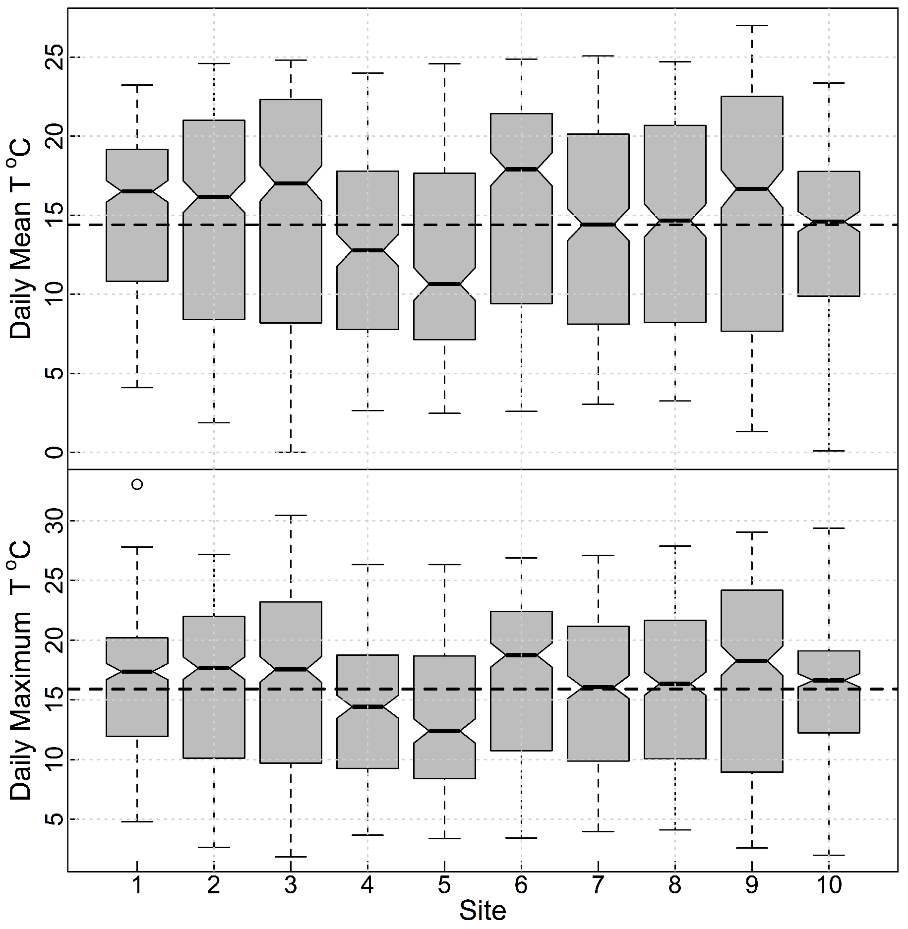
showed significant variation within the watershed (Figure 3). Variation in daily mean T s was similar at all sites (Table 2) with sites 3 and 9 showing the greatest variation in daily mean and daily maximum T s . Site 1 had the lowest variance for daily mean and daily maximum T s . While T s at sites were highly correlated (Table 2), there was no clear trend in correlation as a function of the distance between sites. Site 10 showed the weakest relationship with other sites, but this did not seem to be a function of distance since correlations for site 10 were stronger with site 1 (outlet) than with all other sites in the reach.
Daily mean T s was strongly correlated with daily mean T a at all sites, and daily maximum T s and maximum T a were also strongly correlated at all sites (Table 3). The correlations were significant for all basins for mean temperatures and all basins except basin 10 (where p < 0 . 10 ) for maximum temperatures. Pearson’s correlation coefficients for mean T s and mean R s ranged from 0.0 to 0.50 over the 10 basins, but none of the correlations were significant at the p < 0 . 05 level. Stream temperatures at site 9 indicated the greatest correlation (0.48) with R s , and this site was located at the outlet of Abbott’s Pond that is not shaded and is affected by solar radiation. A relatively high correlation existed at site 7, ρ = 0 . 39 , which is a slow flowing less shaded area of the stream. There were no significant relationships between T s with Q, R H , or V. There was no apparent relationship between P and T s , and there was no difference in the correlation between T a and T s on days with precipitation ( ρ = 0 . 94 ) and days without precipitation ( ρ = 0 . 93 ).
Estimates of slope parameters ( β j ) for regressions on relationships between T s and T a for daily mean and daily maximum showed variation within the watershed (Figure 4, Table 4). The average slope for all sites combined was β a v e = 0 . 61 ± 0 . 11 . The variation in slope parameter for all sites combined was much greater than the slope parameter ( β j ) for each individual site (≈0.01 at all sites). The slope parameters for both mean and maximum T s with T a 
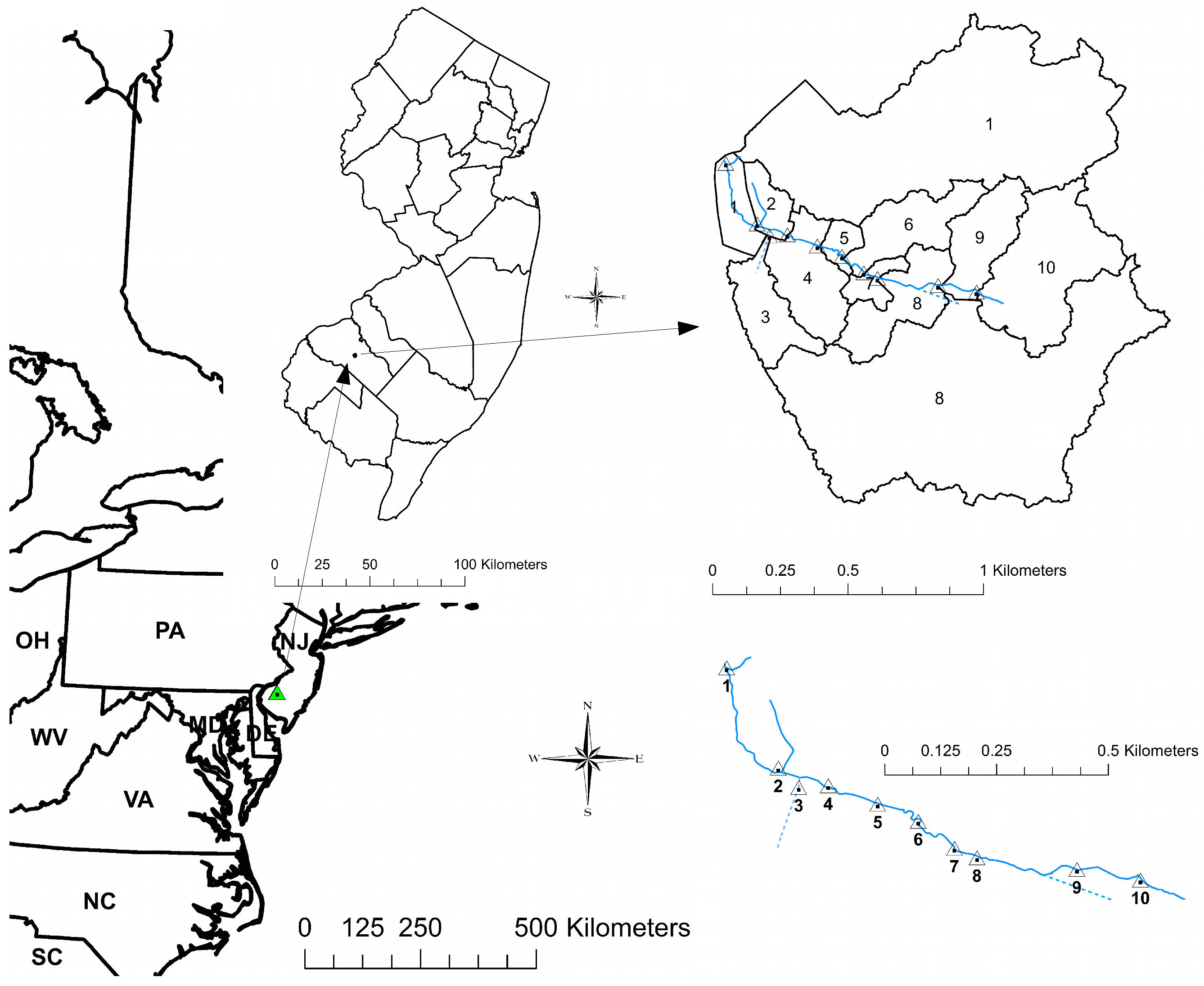
were lowest at sites 1 and 10, representing the outlet and the uppermost section of the watershed, respectively. Slope parameters were largest at sites 3 and 9, which is discussed above. The data logger at site 3 was inside a drainage conduit, which ran under a parking lot, fed from a small retention pond with some wetland vegetation (Figure 2). The retention pond has some shading from low lying wetland vegetation and was lined with large stones.imum) T s for all sites combined. Differences in mean T s between sites can be compared in Table 5. T s differences within ±0.4 C are not considered to be physically significant given the limits of accuracy of the data loggers. Sites 3 and 9 were warmer on average than other sites, and sites 4 and 10 were cooler. The same trends were observed for daily maximum T s for both slope and intercept parameters.
Differences in daily mean temperature between some sites were > 4 C in the summer and > 3 C in the winter (
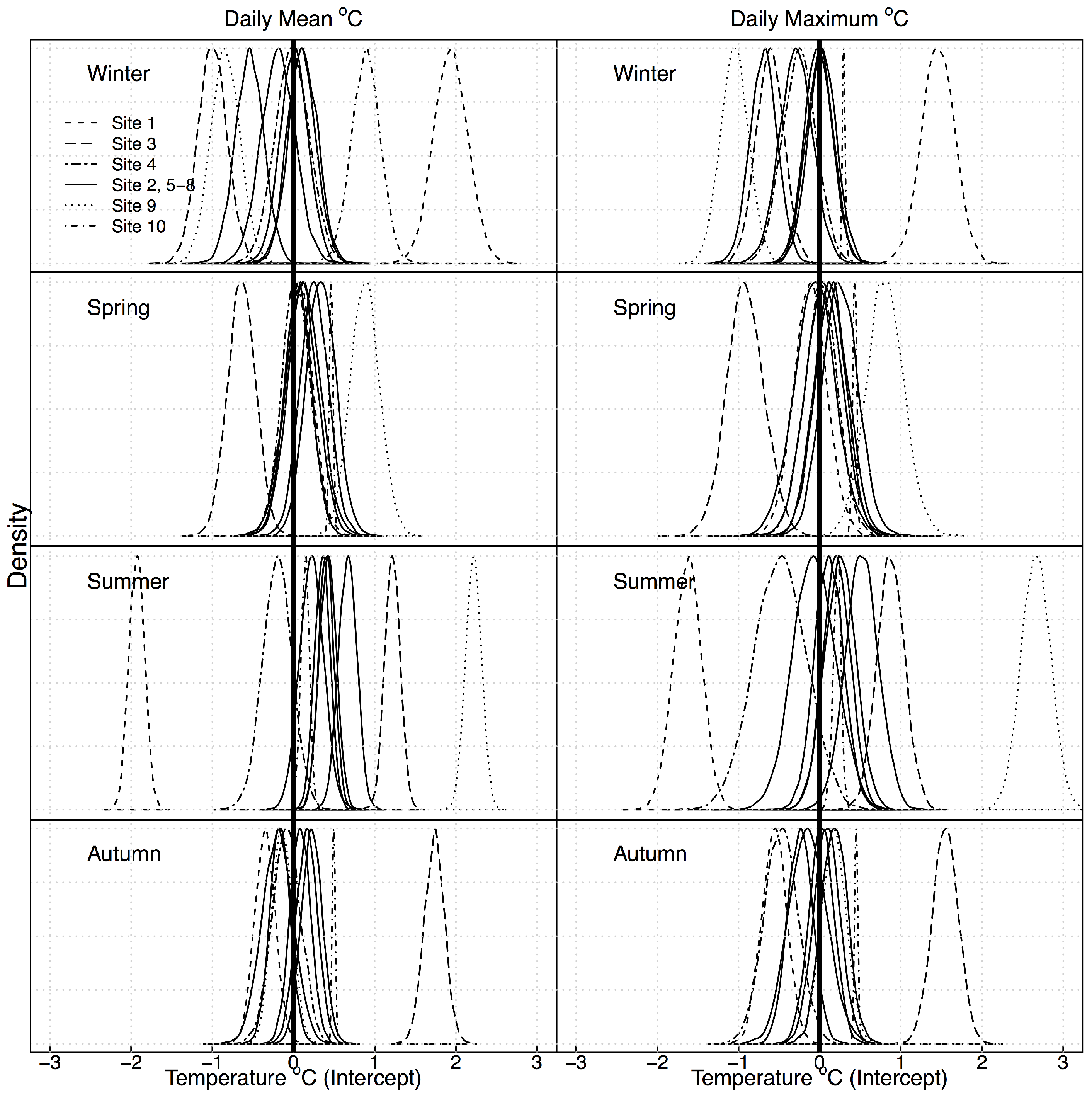
Table 6). There were large temperature differences between sites 9 and 10, which were only 150 m apart, because of the heating that occurred in Abbott’s pond just upstream from site 9. Estimated intercept parameters indicated that mean T s had its greatest variation between sites in the summer within the watershed for both daily mean and daily maximum temperatures (Figure 5), while seasonal mean daily T s and mean daily T a had the least amount of variation in the summer (Table 7). Seasonal mean T s was significantly different ( p < 0 . 05 ) at several sites within the watershed from mean T s for all sites over the entire watershed (Table 6). Mean and maximum daily T s was greater at sites 1 and 10 in the winter, but cooler at these sites in the summer. Site 10 was cooler in spring and autumn as well. Site 9 was warmer in the spring and summer and cooler in the winter compared to other sites. Site 3 was cooler in the winter and spring, but warmer in the summer and autumn. Variation in daily mean and daily maximum T s was greatest in winter and spring overall within sites (width of distributions in Figure 5), and greatest in winter and summer between sites. Daily mean and maximum T s varied more uniformly over the watershed in the spring when T s was more uniform throughout the watershed. Site 10 had the least variation in daily maximum T s in all seasons, and the least variation in daily mean in all seasons except winter compared to all other sites.
Posterior distributions for slope parameters ( β j ) for regressions varied significantly by season (Figure 6). The strongest relationships between T a and T s occurred in the autumn and spring. Relationships were weakest in the winter and summer but showed the greatest variation in summer both within and between sites, contrary to the variation in measured T s . Between site variance was greater than within site variance at all sites in spring, summer and autumn (Figure 6). Sites 1 and 10 showed the weakest relationships with air temperature, and site 9 showed the strongest relationship between daily mean (max) T s and daily mean (max) T a with β = 0 . 74 ± 0 . 02 ( β = 0 . 71 ± 0 . 02 ) for all seasons combined. The weakest relationship with daily mean (max) T a was at site 1 in the summer where β = 0 . 25 ± 0 . 03 ( β = 0 . 19 ± 0 . 04 ).

4. Discussion

The significant variation in daily mean and daily maximum T s within the 1.2 km reach of Chestnut Branch is consistent with results from other small stream networks [35]. Over the entire year, mean daily temperature was similar at all sites except site 10, where mean temperature was just over 1 C cooler. Mean daily temperature was cooler at site 10 compared each of the other sites as well. The slope of the regression line of T s and T a at site 10, β 10 , was significantly lower than at other sites except for site 1 over the entire year. Sites 1 and 10 had the least variation in T s compared with other sites. Furthermore, sites 1 and 10 showed less variation and the greatest temperature differences compared to other sites in winter and summer. These two sites were heavily shaded in the summer and received a greater proportion of flow from groundwater relative to other sites. Site 1 receives inflow from Rowan pond, which is groundwater fed and flows into Chestnut Branch, except at times of high flow. Site 10 was just downstream from where perennial flow begins. These factors help explain the lower variance observed at these sites. For example, Constantz [23] found that variation in T s was 11% in gaining reaches and 30% in losing reaches. Riparian cover tends to moderate diurnal variations and keep maximum temperatures lower than unshaded areas [43,44]. It is not likely that the small differences in flow, apart from the contribution of groundwater, impacted the observed differences in T s . MacDonald et al. [45] found that discharge was important in explaining inter-annual T s variation in a headwater streams, in particular moisture conditions at the watershed scale (10 km 2 ). However, there were no observed relationships between stream flow and T s , and it is not likely that Q impacts T s in Chestnut Branch (2 km 2 ). This is likely due in part to the small size of the watershed, but there is evidence that the duration of temperature exceedance is impacted by stream flow more than daily mean T s [13].
Stream temperature at sites 1 and 10 also showed the weakest relationship (low β ) with T a based on regressions compared with other sites over the entire year and in spring and summer. While lower variance in daily mean T s may indicate the influence of groundwater and/or riparian cover, the weaker relationship with T a indicates that factors other than those that affect T a are controlling T s at these sites. It is likely that interactions with groundwater influx and shading in these reaches impacted the relationship with T a , particularly in the summer. Groundwater temperatures are relatively constant and are close to the average annual air temperature in a region. Stream temperature has been shown to be less responsive to T a in colder tributaries [35], and it seems likely that this is the case within segments of the same stream. Additionally, these sites have dense riparian cover, which leads to a microclimate different that average bulk meteorological conditions. These effects seemed less apparent for maximum temperatures where the means of the slope parameter tended to converge, i.e., less between site variation, for maximum temperature. It seems that relationship of maximum T s with maximum T a is more uniform.
The site with the warmest mean daily temperatures (site 9) had the strongest relationship ( β 9 ) with air temperature, and this site had the greatest variation in daily mean T s . Site 9 was located downstream of the outlet of Abbott’s pond, with little cover, and is most likely to have conditions throughout the year similar to bulk meteorological conditions measured at the weather station. The lack of riparian cover over the pond allows the loss of heat at night to be a function primarily of the temperature gradient between the water and air [46], thus a stronger relationship of T s with T a .
The greatest differences in daily mean T s between sites occurred in the summer. Spatial T s variability between sites was greatest in the summer, and spatial variability of T s was most uniform in winter and spring. Relationships between T a and T s were strongest in spring and autumn and weakest in summer at all sites, but there was greater variability in slope parameters in summer between sites for relationship with T a . These results support the conclusion that micro-climate was more important in the summer when shading can have a larger impact on heat fluxes. For example, Rutherford et al. [47] indicated that differential heating due to absorption of solar radiation by riparian vegetation affects stream temperature. Results indicated a correlation between solar radiation and T s , but correlations were not significant ( p < 0 . 10 ) at all sites. Correlations between T s and R s were greatest at sites 7 and 9. Site 9 was near the outlet of Abbott’s pond, which is clearly impacted by solar radiation, but the correlation at site 7, which was <100 m downstream from site 8 does was not likely physically significant. Micro-climate factors, such as wind speed, relative humidity, and solar radiation, at sites are likely to have effects at these sites, especially in smaller basins and at sheltered sites [48,49]. Bulk measurements for these meteorological variables from a single weather station are less likely to show consistent relationships with T s between sites.
The stronger relationship with T a and higher between site variance in slope parameters in autumn can possibly be explained in part by the major changes in riparian cover that occur during the autumn season. The autumn months were September, October, and November, and leaves are fully shed from trees by mid- to late-October in southern New Jersey. Therefore, autumn represents a time period with both significant cover in some areas and with little cover after leaf fall. Additionally, leaf fall occurs non-uniformly along the stream, which likely impacts heat flux, and the accumulation of leaf litter in the stream varies within the basin. While leaf litter decomposition is an important component for stream metabolism [50] and impacts heat flux in terrestrial systems [51], it is not clear how it impacts stream temperature. Woody debris and small scale morphological features have been shown to increase temperature variability [52], though these factors are not highly variable in Chestnut Branch.
Relative values and variation on slope parameters for relationships of T s and T a provided an indication of the potential that different processes were affecting stream temperature between sites. The 10 sites chosen represented a variety of known conditions along the stream, and the variance in β a v e for regressions using data from all sites within the basin was relatively high compared to variance in β j for each site.
The solar radiation and groundwater inflow were found to have the most significant impact on heat budget in a 116 km 2 watershed in Indiana [53]. Differences at this temporal scale, regressions of T s with T a are able to distinguish stream temperature variations, but, at a season scale, regressions provide more info.
A detailed spatial analysis as described by Isaak et al. [54] was beyond the scope of this study. However, it is likely that differing characteristics between sites were more important in the summer when microclimate is, this is different. Kanno et al. [35] found that T s variability primarily occurred between stream segments as opposed to within a stream segment, i.e., after tributary confluences.

5. Conclusions

The Bayesian hierarchical analysis as applied to the Chestnut Branch watershed provides a straightforward method for identifying local scale variability in the relationship between stream temperature and air temperature. This approach can be applied at relatively small scales to identify areas where different local scale processes may be contributing to the response of stream temperature to different drivers in daily to seasonal time frames. Application of such information can be important for management and conservation of local scale habitat with regard to the potential impacts of land-use and climate change.
Steam temperature variation was lowest at sites with a greater amount of riparian cover that also had a relatively large proportion of flow from groundwater. These sites also showed the weakest relationship between T s and T a , suggesting a significant influence of groundwater influx and shading on the relationship. Stream temperature variation was greatest in the spring and autumn, and lowest in the summer. The relationship between T s and T a varied significantly by season both within and between sites. Relationships were strongest in spring and autumn and weakest in summer at all sites, but greater variability in slope parameters was found between sites in summer. Greater variability in slope parameters and weaker relationships between T s and T a indicate that micro-climate and/or local characteristics of the basin impact T s most in the summer. In general, these results support the conclusion that riparian shading impacts the effect of T a on T s , and that open areas without cover are more likely to have meteorologic conditions similar to bulk conditions. Therefore, T s shows a stronger relationship with measured T a at these sites, though these impacts could not be fully quantified at the daily time scale. Additionally, at the daily scale, the impacts of watershed characteristics and rainfall on T s were not clear. However, this does not imply that these are not important factors affecting T s . Analysis at a finer time resolution is required to quantify these effects, and the posterior distributions for slope parameters will help to locate areas where site-specific factors are more likely to impact T s . The one-minute T s collected and used in this study will be used for further analysis of relationships between T s and other factors, such as land-use/land cover and rainfall, at these sites.

Supplementary Materials

Supplementary material are available online at www.mdpi.com/2306-5338/4/3/44/s1, including R source code for all data analyses.

Acknowledgments

Many undergraduate and graduate students provided vital support without whom this project would not have been completed. Stream gauging was done by John Benigno, Pat Lynch, Chris Wagner, Jason Shaub, Dan Collins and Rob Morrone in Fall 2013 and Spring 2014. T s data collection was done every three weeks and the authors would like to thank Chris Seigel, C. J. Patras, Graham Neville, and Katie Miller for their help on this project. This project was partially funded by Rowan University, and Ken Sears was partially funded through Rowan University’s Thomas N. Bantivoglio Honors Program.

Author Contributions

K.W.S. and J.A.D. conceived and designed the sampling methodology and site locations; K.W.S. performed data collection; J.A.D. and K.W.S. analyzed the data; J.A.D. and A.O.A. wrote the paper and interpreted analysis results.

Conflicts of Interest

The authors declare no conflict of interest. The founding sponsors had no role in the design of the study; in the collection, analyses, or interpretation of data; in the writing of the manuscript, and in the decision to publish the results.

References

  1. Webb, B.W.; Hannah, D.M.; Moore, R.D.; Brown, L.E.; Nobilis, F. Recent advances in stream and river temperature research. Hydrol. Process. 2008, 22, 902–918. [Google Scholar] [CrossRef]
  2. Döll, P.; Zhang, J. Impact of climate change on freshwater ecosystems: A global-scale analysis of ecologically relevant river flow alterations. Hydrol. Earth Syst. Sci. 2010, 14, 783–799. [Google Scholar] [CrossRef] [Green Version]
  3. Hester, E.T.; Doyle, M.W. Human impacts to river temperature and their effects on biological processes: A quantitative synthesis. J. Am. Water Resour. Assoc. 2011, 47, 571–587. [Google Scholar] [CrossRef]
  4. Schindler, D.E.; Rogers, D.E.; Scheuerell, M.D. Effects of changing climate on zooplankton and juvenile sockeye salmon growth in southwestern Alaska. Ecology 2005, 86, 198–209. [Google Scholar] [CrossRef]
  5. Strayer, D.L.; Downing, J.A.; Haag, W.R.; King, T.L.; Layzer, J.B.; Newton, T.J.; Nichols, S.J. Changing perspectives on pearly mussels, North America’s most imperiled animals. BioScience 2004, 54, 429–439. [Google Scholar] [CrossRef]
  6. Caissie, D. The thermal regime of rivers: A review. Freshw. Biol. 2006, 51, 1389–1406. [Google Scholar] [CrossRef]
  7. Ducharne, A. Importance of stream temperature to climate change impact on water quality. Hydrol. Earth Syst. Sci. 2008, 12, 797–810. [Google Scholar] [CrossRef]
  8. Caissie, D.; Satish, M.G.; El-Jabi, N. Predicting water temperatures using a deterministic model: Application on Miramichi River catchments (New Brunswick, Canada). J. Hydrol. 2007, 336, 303–315. [Google Scholar] [CrossRef]
  9. Kaushal, S.S.; Likens, G.E.; Jaworski, N.A.; Pace, M.L.; Sides, A.M.; Seekell, D.; Belt, K.T.; Secor, D.H.; Wingate, R.L. Rising stream and river temperatures in the United States. Front. Ecol. Environ. 2010, 8, 461–466. [Google Scholar] [CrossRef]
  10. Bonacci, O.; Trninić, D.; Roje-Bonacci, T. Analysis of the water temperature regime of the Danube and its tributaries in Croatia. Hydrol. Process. 2008, 22, 1014–1021. [Google Scholar] [CrossRef]
  11. Hawkins, C.P.; Hogue, J.N.; Decker, L.M.; Feminella, J.W. Channel morphology, water temperature, and assemblage structure of stream insects. J. N. Am. Benthol. Soc. 1997, 26, 728–749. [Google Scholar] [CrossRef]
  12. Pandolfo, T.J.; Cope, W.G.; Arellano, C.; Bringolf, R.B.; Barnhart, M.C.; Hammer, E. Upper thermal tolerances of early life stages of freshwater mussels. J. N. Am. Benthol. Soc. 2010, 29, 959–969. [Google Scholar] [CrossRef]
  13. Daraio, J.A.; Bales, J.D.; Pandolfo, T.J. Effects of Land Use and Climate Change on Stream Temperature II: Threshold Exceedance Duration Projections for Freshwater Mussels. JAWRA J. Am. Water Resour. Assoc. 2014, 50, 1177–1190. [Google Scholar] [CrossRef]
  14. Poole, G.C.; Berman, C.H. An Ecological Perspective on In-Stream Temperature: Natural Heat Dynamics and Mechanisms of Human-Caused Thermal Degradation. Environ. Manag. 2001, 27, 787–802. [Google Scholar] [CrossRef]
  15. Garner, G.; Hannah, D.M.; Sadler, J.P.; Orr, H.G. River temperature regimes of England and Wales: Spatial patterns, inter-annual variability and climatic sensitivity. Hydrol. Process. 2014, 28, 5583–5598. [Google Scholar] [CrossRef]
  16. Arscott, D.B.; Tockner, K.; Ward, J.V. Thermal heterogeneity along a braided floodplain river (Tagliamento River, northeastern Italy). Can. J. Fish. Aquatic Sci. 2001, 58, 2359–2373. [Google Scholar] [CrossRef]
  17. Long, S.L.; Jackson, C.R. Variation of stream temperature among mesoscale habitats within stream reaches: Southern Appalachians. Hydrol. Process. 2013, 28, 3041–3052. [Google Scholar] [CrossRef]
  18. DeWeber, J.T.; Wagner, T. A regional neural network ensemble for predicting mean daily river water temperature. J. Hydrol. 2014, 517, 187–200. [Google Scholar] [CrossRef]
  19. Vatland, S.J.; Gresswell, R.E.; Poole, G.C. Quantifying stream thermal regimes at multiple scales: Combining thermal infrared imagery and stationary stream temperature data in a novel modeling framework. Water Resour. Res. 2015. [Google Scholar] [CrossRef]
  20. Letcher, B.H.; Hocking, D.J.; O’Neil, K.; Whiteley, A.R.; Nislow, K.H.; O’Donnell, M.J. A hierarchical model of daily stream temperature using air-water temperature synchronization, autocorrelation, and time lags. Peer J. 2016, 4. [Google Scholar] [CrossRef] [PubMed]
  21. Smith, K.; Lavis, M.E. Environmental influences on the temperature of a small upland stream. Oikos 1975, 26, 228–236. [Google Scholar] [CrossRef]
  22. Matheswaran, K.; Blemmer, M.; Rosbjerg, D.; Boegh, E. Seasonal variations in groundwater upwelling zones in a Danish lowland stream analyzed using Distributed Temperature Sensing (DTS). Hydrol. Process. 2013, 28, 1422–1435. [Google Scholar] [CrossRef]
  23. Constantz, J. Interaction between stream temperature, streamflow, and groundwater exchanges in alpine streams. Water Resour. Res. 1998, 34, 1609–1615. [Google Scholar] [CrossRef]
  24. Brown, L.E.; Hannah, D.M. Spatial heterogeneity of water temperature across an alpine river basin. Hydrol. Process. 2008, 22, 954–967. [Google Scholar] [CrossRef]
  25. Cadbury, S.L.; Hannah, D.M.; Milner, A.M.; Pearson, C.P.; Brown, L.E. Stream temperature dynamics within a New Zealand glacierized river basin. River Res. Appl. 2007, 24, 68–89. [Google Scholar] [CrossRef]
  26. Brown, L.E.; Hannah, D.M.; Milner, A.M. Hydroclimatological influences on water column and streambed thermal dynamics in an alpine river system. J. Hydrol. 2006, 325, 1–20. [Google Scholar] [CrossRef]
  27. Wagner, M.J.; Bladon, K.D.; Silins, U.; Williams, C.H.; Martens, A.M.; Boon, S.; MacDonald, R.J.; Stone, M.; Emelko, M.B.; Anderson, A. Catchment-scale stream temperature response to land disturbance by wildfire governed by surface-subsurface energy exchange and atmospheric controls. J. Hydrol. 2014, 517, 328–338. [Google Scholar] [CrossRef]
  28. Nelson, K.C.; Palmer, M.A. Stream Temperature Surges Under Urbanization and Climate Change: Data, Models, and Responses. JAWRA J. Am. Water Resour. Assoc. 2007, 43, 440–452. [Google Scholar] [CrossRef]
  29. Herb, W.R.; Janke, B.; Mohseni, O.; Stefan, H.G. Thermal pollution of streams by runoff from paved surfaces. Hydrol. Process. 2008, 22, 987–999. [Google Scholar] [CrossRef]
  30. Hannah, D.M.; Malcolm, I.A.; Soulsby, C.; Youngson, A.F. A comparison of forest and moorland stream microclimate, heat exchanges and thermal dynamics. Hydrol. Process. 2008, 22, 919–940. [Google Scholar] [CrossRef]
  31. Djebou, S.D.C.; Singh, V.P. Entropy-Based Index for Spatiotemporal Analysis of Streamflow, Precipitation, and Land-Cover. J. Hydrol. Eng. 2016, 21, 05016024. [Google Scholar] [CrossRef]
  32. Mohseni, O.; Stefan, H.G. Stream temperature/air temperature relationship: A physical interpretation. J. Hydrol. 1999, 218, 128–141. [Google Scholar] [CrossRef]
  33. Johnson, M.F.; Wilby, R.L.; Toone, J.A. Inferring air–water temperature relationships from river and catchment properties. Hydrol. Process. 2014, 28, 2912–2928. [Google Scholar] [CrossRef] [Green Version]
  34. Johnson, S.L. Stream temperature: Scaling of observations and issues for modelling. Hydrol. Process. 2003, 17, 497–499. [Google Scholar] [CrossRef]
  35. Kanno, Y.; Vokoun, J.C.; Letcher, B.H. Paired Stream-Air Temperature Measurements Reveal Fine-Scale Thermal Heterogeneity within Headwater Brook Trout Stream Networks. River Res. Appl. 2013, 30, 745–755. [Google Scholar] [CrossRef]
  36. Rice, K.C.; Jastram, J.D. Rising air and stream-water temperatures in Chesapeake Bay region, USA. Clim. Chang. 2015, 128, 127–138. [Google Scholar] [CrossRef]
  37. Stefan, H.G.; Preud’Homme, E.B. Stream temperature estimation from air temperature. Water Resour. Bull. 1993, 29, 27–45. [Google Scholar] [CrossRef]
  38. Caissie, D.; El-Jabi, N.; Satish, M.G. Modelling of maximum daily water temperatures in a small stream using air temperatures. J. Hydrol. 2001, 251, 14–28. [Google Scholar] [CrossRef]
  39. R Core Team. R: A Language and Environment for Statistical Computing; R Foundation for Statistical Computing: Vienna, Austria, 2014. [Google Scholar]
  40. Sturtz, S.; Ligges, U.; Gelman, A. R2WinBUGS: A Package for Running WinBUGS from R. J. Stat. Softw. 2005, 12, 1–16. [Google Scholar] [CrossRef]
  41. Gelman, A.; Hill, J. Data Analysis Using Regression and Multilevel/Hierarchical Models; Cambridge University Press: Cambridge, UK, 2007. [Google Scholar]
  42. Lunn, D.; Jackson, C.; Best, N.; Thomas, A.; Spiegelhalter, D. The BUGS Book: A Practical Introduction to Bayesian Analysis; Taylor & Francis: Abingdon, UK, 2012. [Google Scholar]
  43. Malcolm, I.A.; Soulsby, C.; Hannah, D.M.; Bacon, P.J.; Youngson, A.F.; Tetzlaff, D. The influence of riparian woodland on stream temperatures: Implications for the performance of juvenile salmonids. Hydrol. Process. 2008, 22, 968–979. [Google Scholar] [CrossRef]
  44. Broadmeadow, S.B.; Jones, J.G.; Langford, T.E.L.; Shaw, P.J.; Nisbet, T.R. The influence of riparian shade on lowland stream water temperatures in southern England and their viability for brown trout. River Res. Appl. 2011, 27, 226–237. [Google Scholar] [CrossRef]
  45. MacDonald, R.J.; Boon, S.; Byrne, J.M.; Silins, U. A comparison of surface and subsurface controls on summer temperature in a headwater stream. Hydrol. Process. 2013, 28, 2338–2347. [Google Scholar] [CrossRef]
  46. Moore, R.D.; Spittlehouse, D.; Story, A. Riparian Microclimate and Stream Temperature Response to Forest Harvesting: A Review. J. Am. Water Resour. Assoc. 2005, 41, 813. [Google Scholar] [CrossRef]
  47. Rutherford, J.C.; Blackett, S.; Blackett, C.; Saito, L.; Davies-Colley, R.J. Predicting the effects of shade on water temperature in small streams. N. Z. J. Marine Freshw. Res. 1997, 31, 707–721. [Google Scholar] [CrossRef]
  48. Benyahya, L.; Caissie, D.; El-Jabi, N.; Satish, M.G. Comparison of microclimate vs. remote meteorological data and results applied to a water temperature model (Miramichi River, Canada). J. Hydrol. 2010, 380, 247–259. [Google Scholar] [CrossRef]
  49. Brown, L.E.; Cooper, L.; Holden, J.; Ramchunder, S.J. A comparison of stream water temperature regimes from open and afforested moorland, (Yorkshire Dales, northern England. Hydrol. Process. 2010, 24, 3206–3218. [Google Scholar] [CrossRef]
  50. Fisher, S.G.; Likens, G.E. Energy Flow in Bear Brook, New Hampshire: An Integrative Approach to Stream Ecosystem Metabolism. Ecol. Monogr. 1973, 43, 421. [Google Scholar] [CrossRef]
  51. Ogée, J.; Lamaud, E.; Brunet, Y.; Berbigier, P.; Bonnefond, J.M. A long-term study of soil heat flux under a forest canopy. Agric. For. Meteorol. 2001, 106, 173–186. [Google Scholar] [CrossRef]
  52. Cardenas, M.B.; Harvey, J.W.; Packman, A.I.; Scott, D.T. Ground-based thermography of fluvial systems at low and high discharge reveals potential complex thermal heterogeneity driven by flow variation and bioroughness. Hydrol. Process. 2008, 22, 980–986. [Google Scholar] [CrossRef]
  53. Younus, M.; Hondzo, M.; Engel, B.A. Stream temperature dynamics in upland agricultural watersheds. J. Environ. Eng. 2000, 126, 518–526. [Google Scholar] [CrossRef]
  54. Isaak, D.J.; Wollrab, S.; Horan, D.; Chandler, G. Climate change effects on stream and river temperatures across the northwest U.S. from 1980–2009 and implications for salmonid fishes. Clim. Chang. 2012, 113, 499–524. [Google Scholar] [CrossRef]
Figure 1. Location of Chestnut Branch. Dashed lines in representation of Chestnut Branch signifies an underground conduit that drains into the stream.
Hydrology 04 00044 g001
Figure 2. Location of sites where stream temperature data were collected.
Hydrology 04 00044 g002
Figure 3. Daily mean (top) and maximum (bottom) stream temperature ( C) at each recording site. Mean daily stream temperature and mean daily maximum stream temperature over the data collection period is represented by the dotted lines.
Hydrology 04 00044 g003
Figure 4. Regression parameters for the relationship between mean daily stream temperatures and mean daily air temperatures (black) and maximum daily stream temperatures and maximum daily air temperatures (greay) at each site. Parameters were estimated using Bayesian regression analyses. Points indicate mean value of regression parameter ( μ β and μ α ), solid lines indicate 67% confidence level, and + indicates 95% confidence level ( σ β and σ α ). Intercept is C where an intercept = 0 C (dark dotted line) indicates that the mean (maximum) daily T s at a basin is the same as the mean (maximum) stream temperature for all basins combined over the period of record. Mean daily and maximum stream temperature was used as the baseline to calculate anomalies for mean daily and mean daily maximum stream temperatures at each basin.
Hydrology 04 00044 g004
Figure 5. Posterior probability density functions of estimated intercept temperature ( C) from daily mean (left) and maximum (right) stream temperature Bayesian hierarchical regression with daily mean and maximum air temperature, respectively, for each season at each recording site. Mean daily and maximum stream temperature for each season was used as the baseline to calculate anomalies for seasonal mean daily and season mean daily maximum stream temperatures at each basin. An intercept = 0 C (dark vertical line) indicates that the mean daily T s at a basin is the same as the mean stream temperature for all basins combined for that season. Winter = DJF, Spring = MAM, Summer = JJA, Autumn = SON.
Hydrology 04 00044 g005
Figure 6. Posterior pdfs (probability density functions) of regression slope parameters ( β ) for the relationship between mean daily stream temperatures and mean daily air temperatures and between daily maximum stream temperature and daily maximum air temperature at each site for each season of the year. Parameters were estimated using Bayesian regression analyses. Relationships of stream temperature with air temperature are relatively uniform between basins in the winter. Posterior pdfs are different at sites 1, 9, and 10 in the summer than for the other sites, and posterior pdfs are more variable in autumn. Winter = DJF, Spring = MAM, Summer = JJA, Autumn = SON.
Hydrology 04 00044 g006
Table 1. Basin characteristics and description of site locations. Length, L, in meters of the location of the site upstream from the stream outlet at site 1. NA indicates that is not a temperature logger upstream of the site. Area, A, in hectares of drainage area for the basin delineated at the location of the logger. Sample size, N, indicating number of days with temperature readings at each site.
SiteL (m)A (ha)NLocation/Description
1064.4316Outlet of the basin, highly shaded reach with intermittent tributaries that flow during rainfall events.
23033.29346Confluence of surface inflow from Rowan Pond, which is shaded most of the day and groundwater fed with a baseflow of approximately 25% of flow in Chestnut Branch.
3376 * 7.17343Drainage conduit that runs under a parking lot and drains a constructed wetland/detention area that primarily collects runoff from student residences on campus. Baseflow in this conduit was estimated to be <0.001 m 3 s 1 with enough flow for the logger to be fully submerged.
44179.35244Shaded area about midway between sites 2 and 5.
55401.92224Incised shaded section of the stream about midway between sites 4 and 6.
66758.34275Midway point of a relatively broad meandering section of the stream with sparse riparian cover. The stream is incised in this area
77942.28299Downstream site 8 in a sparsely shaded, slow flowing, relatively deep reach that receives runoff directly from a large area of impervious surface.
885279.1302Downstream of shaded riparian area with multiple storm drainage inlets fed from off campus areas of Glassboro.
910907.93330Downstream of Abbott’s Pond, which is surface water fed and not well shaded.
10124618.75330Upstream most section of Chestnut Branch open to atmosphere.
* Not on the main stem of Chestnut Branch.
Table 2. Matrix for comparison of mean daily, daily maximum, and variance of stream temperature (bold), and correlations between sites.
Site 12345678910
Mean CVariance/Correlation, Daily Mean Stream Temperature
115.123.4
214.70.9744.0
315.20.960.9752.9
412.80.980.990.9631.8
512.30.970.990.960.9939.0
615.50.980.990.970.990.9942.8
714.40.980.990.970.990.991.0041.7
814.40.980.990.970.990.990.990.9940.5
915.10.960.990.950.970.980.980.980.9855.9
1013.40.9480.9180.8980.900.890.920.910.910.9029.6
Mean CVariance/Correlation, Daily Maximum Stream Temperature
116.325.2
216.10.9642.3
316.50.940.9649.1
414.10.980.990.9530.1
513.70.960.990.960.9937.0
616.70.960.990.970.990.9940.6
715.70.960.990.960.990.990.9939.9
815.70.960.990.970.990.990.990.9939.0
916.70.950.980.940.970.980.980.980.9859.7
1015.40.890.890.870.870.880.890.880.890.8728.7
Table 3. Pearson’s correlation coefficients ( ρ ) for relationships of daily mean stream temperature and daily mean air temperature, daily maximum stream temperature and daily maximum air temperature, and daily mean stream temperature and daily mean solar radiation.
BasinDaily Mean CDaily Maximum CMean Radiation (Wm 2 )
10.95 *0.91 *0.06
20.96 *0.95 *0.22
30.92 *0.91 *0.15
40.95 *0.93 *0.27
50.95 *0.94 *0.004
60.97 *0.95 *0.30 **
70.96 *0.94 *0.39 **
80.96 *0.95 *0.31 **
90.95 *0.94 *0.48 **
100.90 *0.88−0.07
All0.94 *0.92 *0.18
* significant at p < 0.05; ** significant at p < 0.10.
Table 4. Estimated slope parameter ( β j ) at each site j standard deviation (italics), and estimated β j for each site for the given season and standard deviation (italics).
SiteAll12345678910
Estimated Slope Parameter ( β j )
β a l l 0.610.470.650.680.570.610.640.630.620.720.48
σ β 0.110.010.010.010.010.010.010.010.010.010.01
β W i n t e r 0.300.270.300.320.300.310.300.300.300.290.29
σ β W i n t e r 0.020.030.020.020.020.020.020.020.020.020.02
β S p r i n g 0.510.430.530.520.500.520.530.520.500.560.46
σ β S p r i n g 0.050.020.020.020.020.020.020.020.020.020.02
β S u m m e r 0.330.270.390.320.340.350.350.350.340.440.14
σ β S u m m e r 0.090.040.040.050.050.050.040.040.040.050.05
β A u t u m n 0.580.480.620.490.560.600.610.610.600.750.49
σ β A u t u m n 0.100.020.020.020.030.020.020.020.020.020.02
Table 5. Mean daily temperature anomaly ( C) at each site. Diagonal of matrix (bold) is the temperature anomaly for the site based on all sites combined. Other values are the difference of the mean daily temperature anomaly between each site. Positive values indicate that the mean daily temperature at the site listed in the column is greater than the site listed in the row (all sites combined for bold values). All values were statistically significant ( p < 0 . 001 ); however, differences within ±0.4 C are not considered physically significantly different due to the error in the data loggers.
Site12345678910
Difference in Mean Daily Stream Temperature C
1 0 . 06
20.12 0 . 18
3−0.32−0.44 0 . 26
40.290.170.61 0 . 34
50.200.090.52−0.08 0 . 26
6−0.22−0.340.10−0.51−0.43 0 . 16
7−0.25−0.360.07−0.53−0.45−0.02 0 . 19
8−0.16−0.280.16−0.44−0.360.060.09 0 . 10
9−0.40−0.52−0.08−0.69−0.61−0.18−0.15−0.24 0 . 34
101.090.971.410.800.881.311.331.241.49 1 . 15
Table 6. Mean daily temperature anomaly ( C) at each site for each season. Diagonal of matrix (bold) is the temperature anomaly for the site based on all sites combined. Other values are the difference of the mean daily temperature anomaly between each site. Positive values indicate that the mean daily temperature at the site listed in the column is greater than the site listed in the row (all sites combined for bold values). All values were statistically significant ( p < 0 . 001 ); however, differences within ±0.4 C are not considered physically significantly different due to the error in the data loggers.
Site12345678910
Difference in Mean Daily Stream Temperature C
Winter
12.00
22.48 0 . 48
32.930.46 0 . 94
41.95−0.53−0.980.04
51.93−0.55−1.00−0.020.06
62.12−0.35−0.810.170.20 0 . 13
71.84−0.64−1.09−0.11−0.09−0.280.15
81.82−0.66−1.12−0.14−0.11−0.31−0.020.18
92.780.30−0.160.820.850.650.940.96 0 . 78
101.04−1.43−1.89−0.91−0.88−1.08−0.80−0.77−1.730.95
Spring
1 0 . 02
20.01 0 . 03
30.710.69 0 . 73
40.040.02−0.67 0 . 06
5−0.04−0.06−0.75−0.080.03
6−0.05−0.06−0.75−0.08−0.000.03
7−0.27−0.28−0.98−0.31−0.23−0.220.25
8−0.18−0.20−0.89−0.22−0.14−0.140.080.17
9−0.81−0.82−1.52−0.85−0.77−0.76−0.54−0.630.79
101.091.080.381.051.131.141.361.281.90 1 . 11
Summer
1 2 . 29
2−2.330.04
3-3.15−0.820.86
4−1.730.601.42 0 . 55
5−2.150.181.00−0.42 0 . 13
6−2.290.050.86−0.56−0.13 0 . 00
7−2.60−0.260.55−0.87−0.44−0.310.31
8−2.35−0.020.80−0.62−0.20−0.070.240.06
9 4 .15−1.81−1.00−2.42−1.99−1.86−1..55−1.791.86
101.253.584.402.983.403.533.843.605.39 3 . 54
Autumn
1 0 . 29
2−0.18 0 . 11
3−2.09−1.901.80
4−0.26−0.081.82 0 . 03
5−0.150.031.930.11 0 . 14
6−0.43−0.251.65−0.17−0.280.14
7−0.58−0.391.51−0.31−0.42−0.140.29
8−0.51−0.331.57−0.25−0.36−0.080.060.22
9−0.21−0.021.880.05−0.050.230.370.31 0 . 08
100.941.133.031.201.101.381.521.461.15 1 . 23
Table 7. Mean and variance of the mean daily air temperature and mean daily maximum air temperature over the period of data collection.
Daily T CSDMaximum T CSD
Winter
Air0.616.205.496.67
Water6.562.628.072.67
Spring
Air10.57.3216.07.77
Water12.44.1014.34.07
Summer
Air23.31.8529.02.41
Water21.91.9223.22.28
Autumn
Air14.76.6920.37.12
Water16.84.2518.04.25

