Abstract
It is always a dream of hydrologists to model the mystery of complex hydrological processes in a precise way. If parameterized correctly, a simple hydrological model can represent nature very accurately. In this study, a simple and effective optimization algorithm, sequential replacement of weak parameters (SRWP), is introduced for automatic calibration of hydrological models. In the SRWP algorithm, a weak parameter set is sequentially replaced with another deeper and good parameter set. The SRWP algorithm is tested on several theoretical test functions, as well as with a hydrological model. The SRWP algorithm result is compared with the shuffled complex evolution-University of Arizona (SCE-UA) algorithm and the robust parameter estimation (ROPE) algorithm. The result shows that the SRWP algorithm easily overcomes the local minima and converges to the optimal parameter space. The SRWP algorithm does not converge to a single optima; instead, it gives a convex hull of an optimal space. An ensemble of results can be generated from the optimal space for prediction purpose. The ensemble spread will account for the parameter estimation uncertainty. The methodology was demonstrated using the hydrological model (HYMOD) conceptual model on upper Neckar catchments of southwest Germany. The results show that the parameters estimated by this stepwise calibration are robust and comparable to commonly-used optimization algorithms. SRWP can be an alternative to other optimization algorithms for model calibration.
1. Introduction
Over the last few decades, a number of conceptual hydrological models that represent complex hydrological processes have emerged. They are increasingly used due to the simplicity of implementation. All of the hydrological models have a certain number of parameters; some of them have a physical meaning, while others do not. An important step in applying these models is the need to estimate the parameters using observed data before using the model for practical purposes. The typical way to estimate the parameters is by adjusting the parameters values by various means, so that the response of the model approximates, as closely and consistently as possible, the observed behavior of the catchment [1]. Numerous techniques have been developed to estimate the parameters of a hydrological model. Generally, there are two types of model calibration. First is manual calibration, which relies completely on expert knowledge. Manual calibration can be extremely labor intensive and difficult to implement for complex model calibration situations where models are calibrated to long time series of measured data; hence, it can only be useful as a learning exercise for modelers [2]. The other method is automatic calibration, which employs the power, ability to follow systematic programmed rules, speed and capability of the computer [1,3]. This can be used for any complex model calibration situation.
In manual calibration, agreement between simulated and observed hydrographs is usually subjective and based on visual comparison. The parameters are tuned based on the expert guesses. Automatic calibration can use different single or multi-objective functions for parameter adjustments, and different criteria can be used for the evaluation of the goodness of fit between observed and modeled hydrographs. Parameterization is a challenging task due to the fact that different parameter vectors that control the model’s physical processes’ description might have the same effect on the discharge generation [4,5]. There are several local and global optimization algorithms available. Some of the algorithm results depend on initial guesses and can get trapped in local minima or maxima. To overcome such problems, global optimization algorithms, like shuffled complex evolution-University of Arizona (SCE-UA), simulated annealing (SA), the genetic algorithm (GA), etc., have emerged [6].
Parameter estimation of hydrological models has been receiving increased attention from the hydrology and land surface modeling community [1,4,5,6,7,8,9,10,11,12,13,14,15,16] and many more. Following the same trend, in this current study, a simple parameter estimation technique is presented to solve and understand the problem associated with parameter estimation of hydrological models.
In this study, the concepts of geometry and multivariate statistics are used to address the problem associated with parameter estimation in hydrological models. Specifically, convex sets and the depth function defined in Tukey [17] are used as a tool. Bárdossy and Singh [5], Singh and Bárdossy [18] and Singh [19] have previously used convex sets and the depth function for model calibration. This paper is the continuation of the work done by Bárdossy and Singh [5] for robust parameter estimation for hydrological models. Here, the goal is not to find the parameter vectors that perform best for the calibration period, but to find parameter vectors that:
- lead to good model performance over the selected time period of prediction;
- lead to a hydrologically-reasonable representation of the corresponding hydrological processes;
- are within the optimal parameter space (small changes of the parameters should not lead to very different results);
- are transferable; they perform well for other time periods and might also perform well for other catchments.
The main objective of the proposed method is to fulfill all of the general requirements of a model calibration (as mentioned above) and also to have a reduction in computational time and to get the optimal space of the parameter set. The algorithm is tested on several theoretical test functions, as well as with a hydrological model. The SRWP algorithm results are compared with the shuffled complex evolution-University of Arizona (SCE-UA) algorithm and the robust parameter estimation (ROPE) algorithm.
2. Methodology
The SRWP algorithm uses the data depth function for the generation of new parameter sets. A brief description of the data depth function and its uses for the SRWP algorithm is explained below.
2.1. Depth Function and Parameters
Data depth is a quantitative measurement of how central a point is with respect to a dataset or a distribution. This helps to define the order (so-called central-outward ordering) and ranks of multivariate data. Depth functions were first introduced by Tukey [17] to identify the center (a kind of generalized median) of a multivariate dataset. Several generalizations of this concept have been defined since [20,21,22]. The points with high depth are the points that lie in the interior of the data cloud, while those with low depth lie near the side of the set and can be seen as unusual in nature. Several types of data depth functions have been developed. For example, the half space depth function, L1depth function, Mahalanobis depth function, Oja median, convex hull peeling depth function and simplicial median. For more detailed information about data depth functions and their uses, please refer to [5,20,23]. The methodology presented in this study is not affected by the choice of data depth function. Tukey’s half space depth is one of the most popular depth functions available, and it is conceptually simple and satisfies several desirable properties of depth functions [24]. Hence, in this study, the half space data depth function was used.
The half space depth of a point, p, with respect to the finite set X in the ddimensional space is defined as the minimum number of points of the set X lying on one side of a hyperplane through the point p. The minimum is calculated over all possible hyperplanes. Formally, the half space depth of the point p with respect to set X (both in the d dimensional space) is:
Here, is the scalar product of the d dimensional vectors and is an arbitrary unit vector in the d dimensional space representing the normal vector of a selected hyperplane.
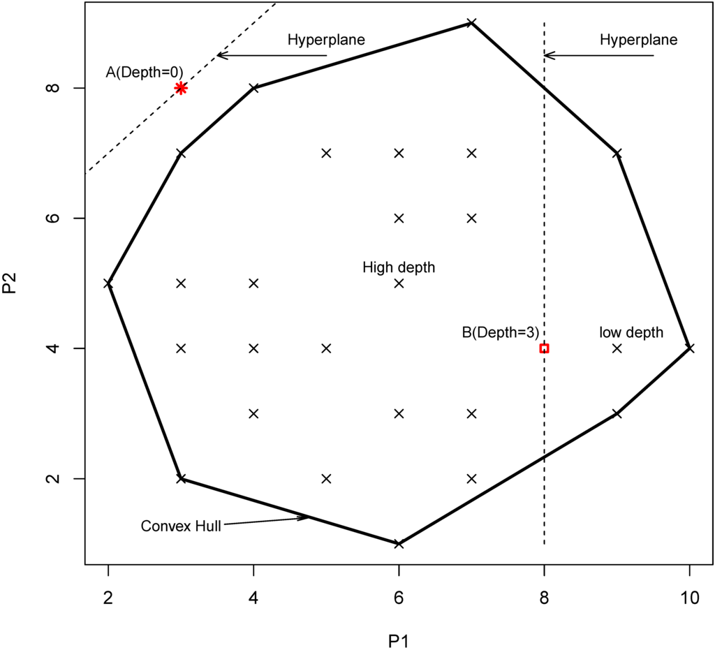
Figure 1.
Example of convex hull, high and low depth in the two-dimensional case (P1 and P2 are two parameters of a model. The red star (A) is a point with depth 0 and red square (B) is a point with depth 3).
Figure 1.
Example of convex hull, high and low depth in the two-dimensional case (P1 and P2 are two parameters of a model. The red star (A) is a point with depth 0 and red square (B) is a point with depth 3).

If the point p is outside the convex hull of X, then its depth is 0. The convex hull of a set of points S is the smallest area polygon that encloses S. Points on and near the boundary of the convex hull have low depth, while points deep inside have high depth. Let P1 and P2 be two parameters of any model. Figure 1 shows the example of a convex hull with low and high depth. The combination of parameters P1 and P2 makes a parameter set. The parameter set that is more central in the parameter space has higher depth. One advantage of this depth function is that it is invariant to affine transformations of the space. This means that the different ranges of the parameters have no influence on their depth. These properties of data depth functions are very useful for hydrological model calibration. This is simply because hydrological model parameters vary in their range and scale. Application of the data depth function is relatively new in the field of water resources. The first application of data depth functions in the field of water resources was seen in the year 2008 by Chebana and Ouarda [23]. They used a depth function to identify the weights of a non-linear regression for flood estimation. In order to identify robust parameters for hydrological models, the statistical concept of data depth was first used by Bárdossy and Singh [5]. They used the data depth function to study the geometrical properties of hydrological model parameters and developed the ROPE algorithm. Singh and Bárdossy [18] used the data depth function for the identification of critical events and developed the ICEalgorithm. Singh et al. [25] used the data depth function for defining predictive uncertainty. Recently, Singh et al. [26] used the data depth function for improving the training of an artificial neural network model.
Bárdossy and Singh [5] demonstrated that the parameters having higher depths are robust in the sense of sensitivity (small change in the parameters’ values) and transferability to other time periods. In this study, the idea of the geometrical properties of the parameters is extended, and a new algorithm for hydrological model parameter estimation is developed. For details about the geometrical properties of the model parameters, please refer to Bárdossy and Singh [5].
2.2. Sequential Replacement of Weak Parameters Algorithm
The ROPE algorithm was further modified and improved by sequential replacement of the weak parameter set with another deeper and good parameter set. A Monte Carlo simulation was performed using a wide range of parameters, and the upper N percentage of well-performing parameters were taken to form a boundary/domain of parameter space. A new parameter was generated in the defined domain, such that the depth of the parameter set is greater than zero in that domain. The performance of this generated parameter set was calculated. If the performance of this newly generated parameter set were better than the minimum performance within a predefined domain, then it was replaced with a newly generated parameter set. This step-wise procedure was repeated until the difference between the maximum and minimum performance in the domain of the parameter space was minimal and acceptable for the purpose of modeling. A general description of the SRWP method is given below. Furthermore, Figure 2 illustrates the methodology.
- Generate N parameter sets from a uniform distribution in the feasible parameter space.
- Compute the objective function at each parameter set.
- Sort the parameter sets in order of increasing or decreasing criteria based on the goal (minimize or maximize)
- Select the best m percentage parameter set and make a convex hull.
- Generate a new parameter set, such that its depth > 0, and compute the objective function for this parameter set.
- If the value of the objective function is better than the worst criterion in the convex hull, replace the corresponding parameter set with the newly-generated parameter set. Otherwise, repeat Steps 5 and 6 until there is no change in the volume of the convex hull or the minimum performance is satisfied.
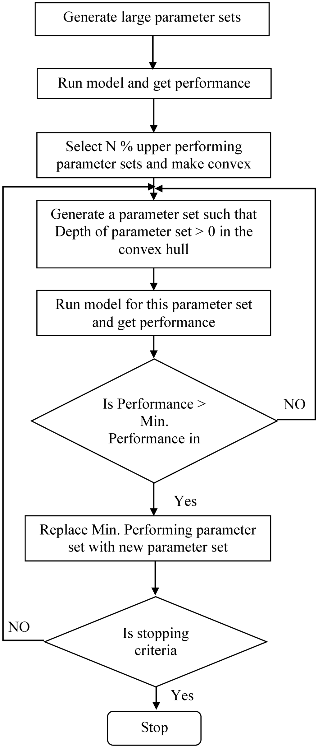
Figure 2.
Schematical explanation of the sequential replacement of weak parameters algorithm.
Figure 2.
Schematical explanation of the sequential replacement of weak parameters algorithm.

This algorithm does not converge to a single best parameter set (which may not exist). Instead it gives a convex hull of parameters, where all of the parameters are equally good. This simply means that it is an optimal parameter space where objective functions are very similar. Once the optimal space is obtained, for real-world applications, the model can be run for many parameter sets from the optimal space, and the results can be given as an ensemble. The spread of the ensemble will account for the parameter uncertainty. Alternatively, the deepest parameter set from the optimal space can be used for prediction purposes. This algorithm can be applied to any performance measures or objective functions. The SRWP algorithm increases the sample of the parameter sets with higher relative depth with the aim of obtaining parameter sets that are robust with respect to changing the period of simulation.
The basic difference between the SRWP and ROPE algorithm is that the SRWP algorithm utilizes Monte Carlo simulation initially to generate numerous candidates in the defined domain of the parameter range, and then, the data depth function is used to get a new parameter set. The candidates with “worst” performances are replaced with those with “better” performances. Whereas in the ROPE algorithm, the optimal parameter space is reached by the help of the convex hull. In each iteration, a convex hull is created and moved towards the optimal space. Whereas in SRWP, we are filtering out the worst parameters with better performing ones. Hence, the SRWP algorithm can move faster toward the optimal space. The stopping criteria for the SRWP algorithm are very flexible compared to the ROPE algorithm. Optimization can be stopped based on the purpose of the modeling and required accuracy.
3. Case Study
3.1. Test of the SRWP Algorithm on Test Functions
The methodology was tested on some of the well-known simple to complex theoretical test functions [27,28]. These functions are the McCormick function, Levy function, Styblinski–Tang function, Leorn function, Giunta function, Rastrigin function and six-hump camel back function. Details about the test functions and their properties are given in the Appendix. For all seven test functions given in the Appendix, the SRWP algorithm was used to obtain the theoretical optima. The SRWP method succeeded in all of the cases. In all of the cases, the SRWP methods have converged to the optimal space. The beauty of this SRWP method is that it does not converge to a single value; instead, it gives the optimal region or optimal parameter space. Table 1, Table 2, Table 3, Table 4 and Table 5, show the analytical solution of some simple to complex theoretical test functions and the solution obtained by the SRWP algorithm. From the table, we can see that the SRWP algorithm has given very similar results to those obtained analytically. Figure 3, Figure 4, Figure 5 and Figure 6 show the contour map of the test function and optimal space mapped by the SRWP method. It can be seen from the figures that the SRWP method has successfully mapped out the optimal space at different levels of complexity of the function (single optimal space to multiple optimal spaces). The theoretical optimal value is a subset of the optimal space. We can see from the function map of the Rastrigin function that it has different levels of optimal space. The contour map of the Rastrigin map with optimal points shown in Figure 3 shows that the SRWP algorithm is successfully able to map the optimal space, as the concentration of the points are more in the optimal space. Similarly, the six-hump camel back function has two optimal spaces, and the optimal parameter points obtained by the SRWP algorithm have a higher concentration in the two optimal spaces; hence, the SRWP algorithm has successfully mapped both of the optimal spaces. Similar results were obtained for all of the other functions (figure not shown). Hydrological model parameter calibration is also complex, nonlinear and multimodal in nature. Hence, we believe SRWP can perform equally well as it performed on the theoretical functions.

Table 1.
McCormick function, its theoretical solution and the solution from the SRWP algorithm. Std, standard deviation.
| Optimal X | SRWP | Optimal Function | Abs.ERin function | |||
|---|---|---|---|---|---|---|
| X | value | value | value | value | ||
| Avg | −0.54725 | Avg | 0.00016 | |||
| −0.54719 | Max | −0.53530 | −1.9133 | Max | 0.00020 | |
| Min | −0.55910 | Min | 0.00010 | |||
| Std | 0.00602 | Std | 0.00005 | |||
| Avg | −1.54731 | Range | Max | Min | ||
| −1.54719 | Max | −1.53540 | 4 | −1.5 | ||
| Min | −1.55910 | 4 | −3 | |||
| Std | 0.00597 | |||||
Table 2.
Leon function, its theoretical solution and the solution from the SRWP algorithm.
| Optimal X | SRWP | Optimal Function | Abs.ER in function | |||
|---|---|---|---|---|---|---|
| X | value | value | value | value | ||
| Avg | 0.99982 | Avg | 0.00007 | |||
| 1 | Max | 1.01190 | 0 | Max | 0.00010 | |
| Min | 0.98790 | Min | 0.00000 | |||
| Std | 0.00602 | Std | 0.00005 | |||
| Avg | 0.99964 | Range | Max | Min | ||
| 1 | Max | 1.02390 | 1.2 | −1.2 | ||
| Min | 0.97600 | 1.2 | −1.2 | |||
| Std | 0.01210 | |||||
Table 3.
Giunta function, its theoretical solution and the solution from the SRWP algorithm.
| Optimal X | SRWP | Optimal Function | Abs.ER in function | |||
|---|---|---|---|---|---|---|
| X | value | value | value | value | ||
| Avg | 0.46729 | Avg | 0.00420 | |||
| 0.45834282 | Max | 0.47230 | 0.0602472184 | Max | 0.00420 | |
| Min | 0.46240 | Min | 0.00420 | |||
| Std | 0.00249 | Std | 0.00000 | |||
| Avg | 0.46735 | Range | Max | Min | ||
| 0.45834282 | Max | 0.47230 | 1 | −1 | ||
| Min | 0.46230 | 1 | −1 | |||
| Std | 0.00254 | |||||
Table 4.
Styblinski–Tang function, its theoretical solution and the solution from the SRWP algorithm.
| Optimal X | SRWP | Optimal Function | Abs.ER in function | |||
|---|---|---|---|---|---|---|
| X | value | value | value | value | ||
| Avg | −2.90349 | Avg | 0.00007 | |||
| −2.903534 | Max | −2.89830 | −78.332 | Max | 0.00010 | |
| Min | −2.90870 | Min | 0.00000 | |||
| Std | 0.00313 | Std | 0.00005 | |||
| Avg | −2.90348 | Range | Max | Min | ||
| −2.903534 | Max | −2.89840 | 5 | −5 | ||
| Min | −2.90880 | 5 | −5 | |||
| Std | 0.00308 | |||||
Table 5.
Levy function, its theoretical solution and the solution from the SRWP algorithm.
| Optimal X | SRWP | Optimal Function | Abs.ER in function | |||
|---|---|---|---|---|---|---|
| X | value | value | value | value | ||
| Avg | 1.00034 | Avg | 0.00790 | |||
| 1 | Max | 1.01350 | 0 | Max | 0.01640 | |
| Min | 0.98670 | Min | 0.00000 | |||
| Std | 0.00695 | Std | 0.00474 | |||
| Avg | 0.99981 | Range | Max | Min | ||
| 1 | Max | 1.10710 | 10 | −10 | ||
| Min | 0.89160 | 10 | −10 | |||
| Std | 0.05415 | |||||
3.2. Case Study on the Hydrological Model
The concept of this paper will be illustrated with examples from the Neckar catchment. The hydrological model chosen is a modified version of the HYMOD model. A short description of the catchment and the model is provided in this section.
3.2.1. Study Area
This study was carried out on the upper Neckar Basin in southwest Germany in the state of Baden-Württemberg using data from the period 1961–2000. The upper Neckar Basin is characterized by strong variation in altitude between the foot hills of the Black forest in the west, the Neckar River Valley in the center and the steep ascent to the Swabian Alb in the east. The study area elevations range from 238 m a.s.l.–1010 m a.s.l. The 4000 km2 Upper Neckar Basin was subdivided into 13 sub-catchments based on gauging stations (Figure 7). Three of the headwater sub-catchments (Rottweil (Neckar), Tübingen( Steinlach) and Süssen (Fils)) were used for this study.
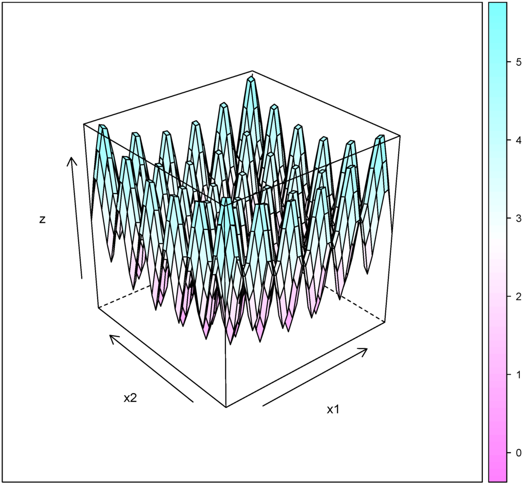
Figure 3.
Rastrigin function.
Figure 3.
Rastrigin function.

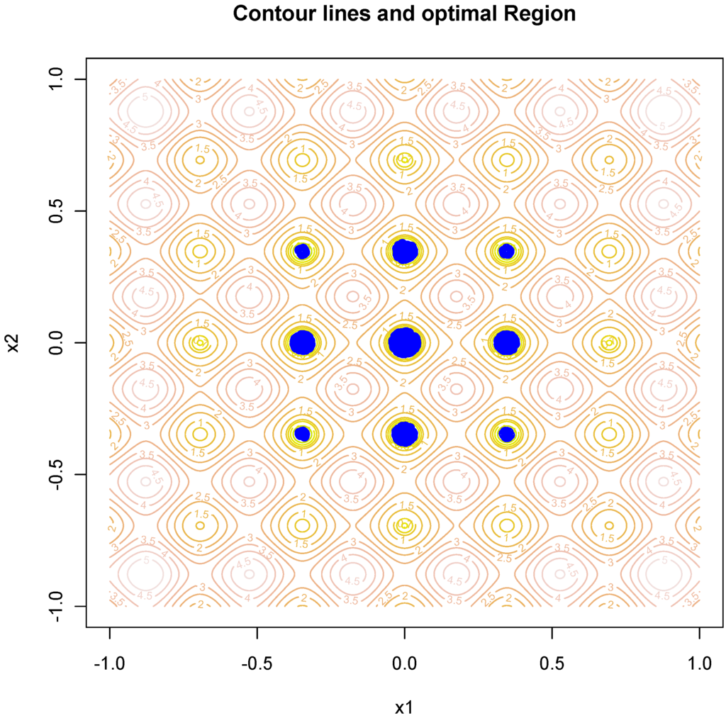
Figure 4.
Contour map for the Rastrigin function and the optimal space obtained by the SRWP algorithm.
Figure 4.
Contour map for the Rastrigin function and the optimal space obtained by the SRWP algorithm.
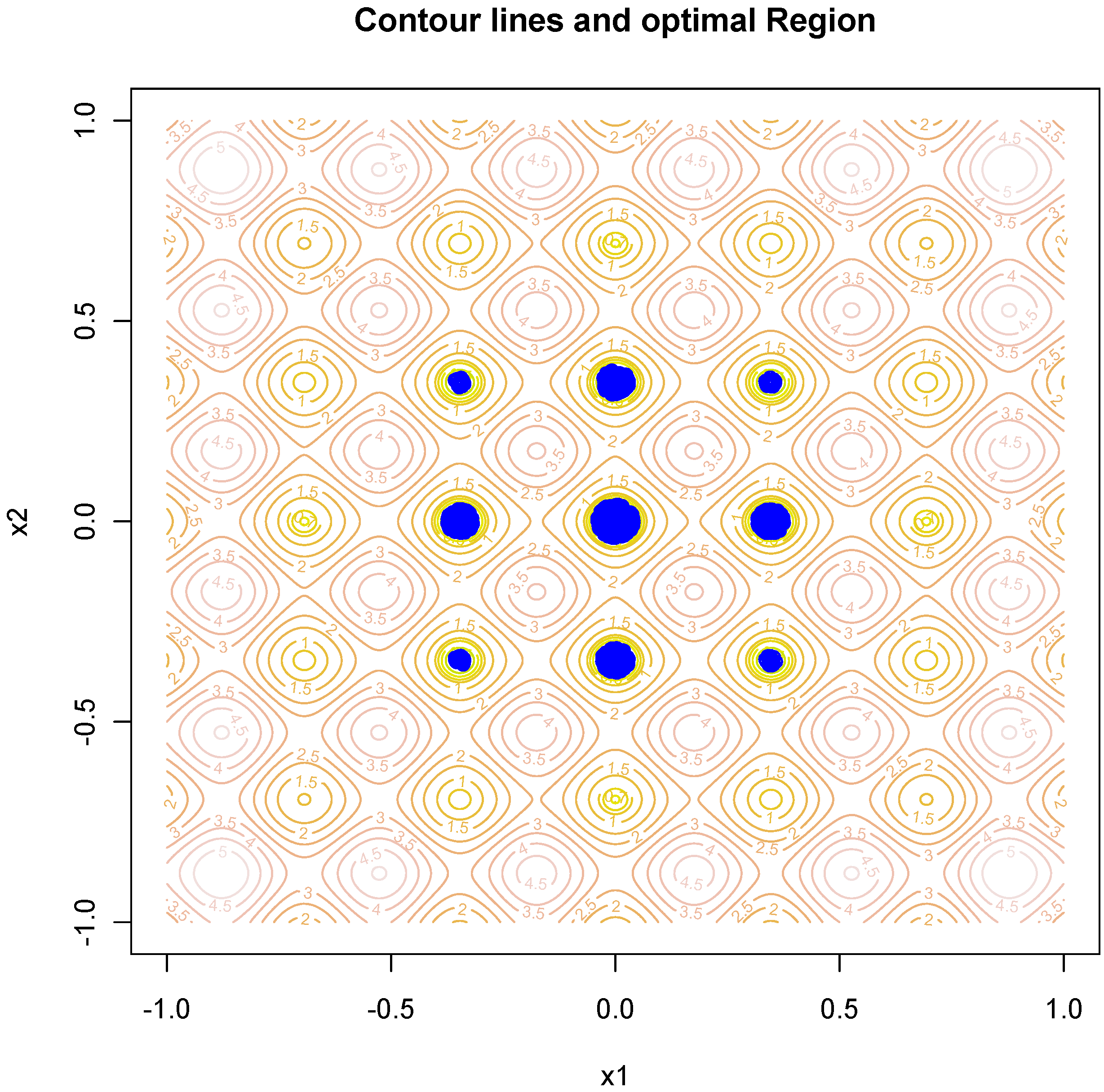

Figure 5.
Six-hump camel back function.
Figure 5.
Six-hump camel back function.
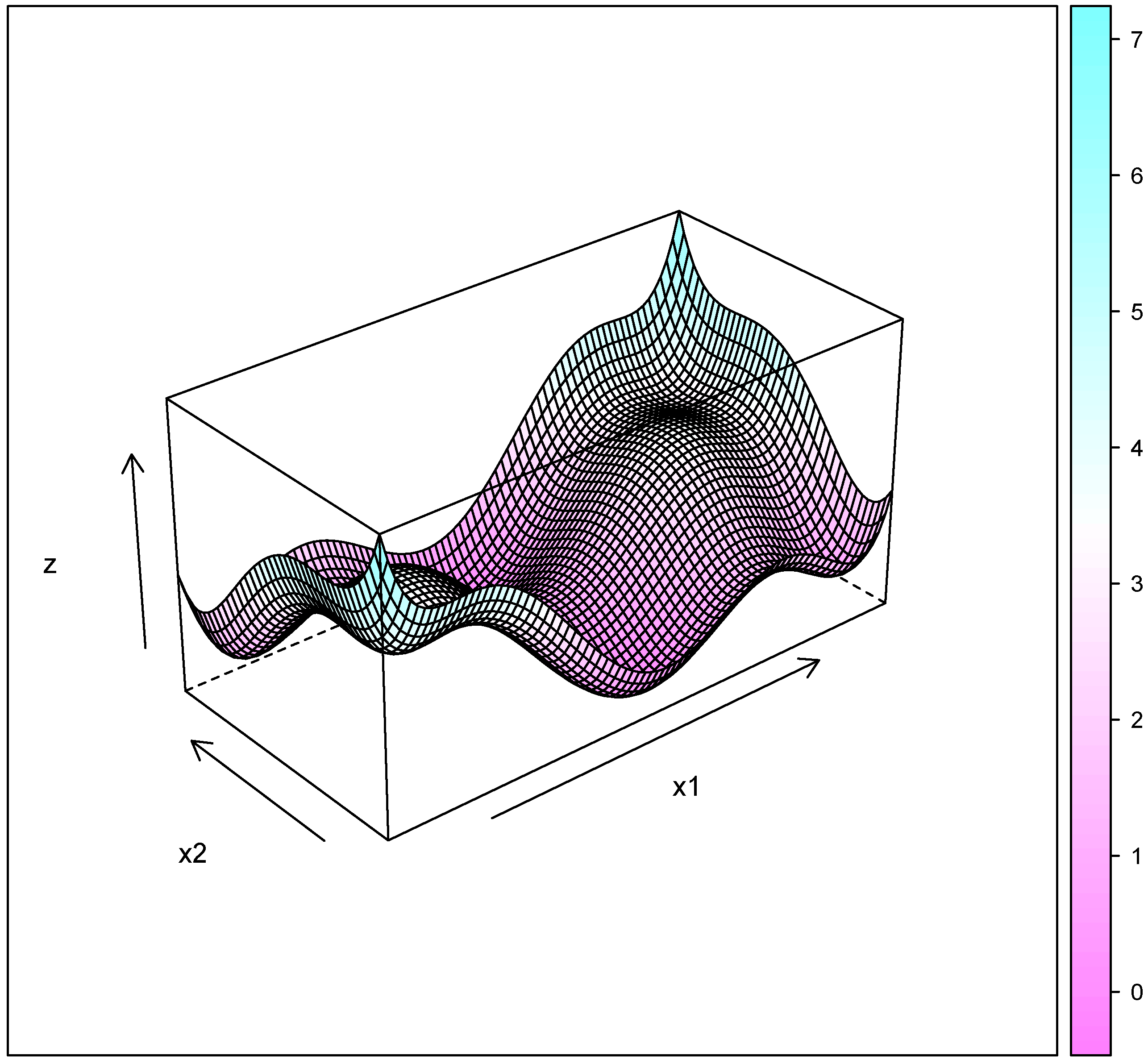

Figure 6.
Contour map for the six-hump camel back function and the optimal space obtained by the SRWP algorithm.
Figure 6.
Contour map for the six-hump camel back function and the optimal space obtained by the SRWP algorithm.
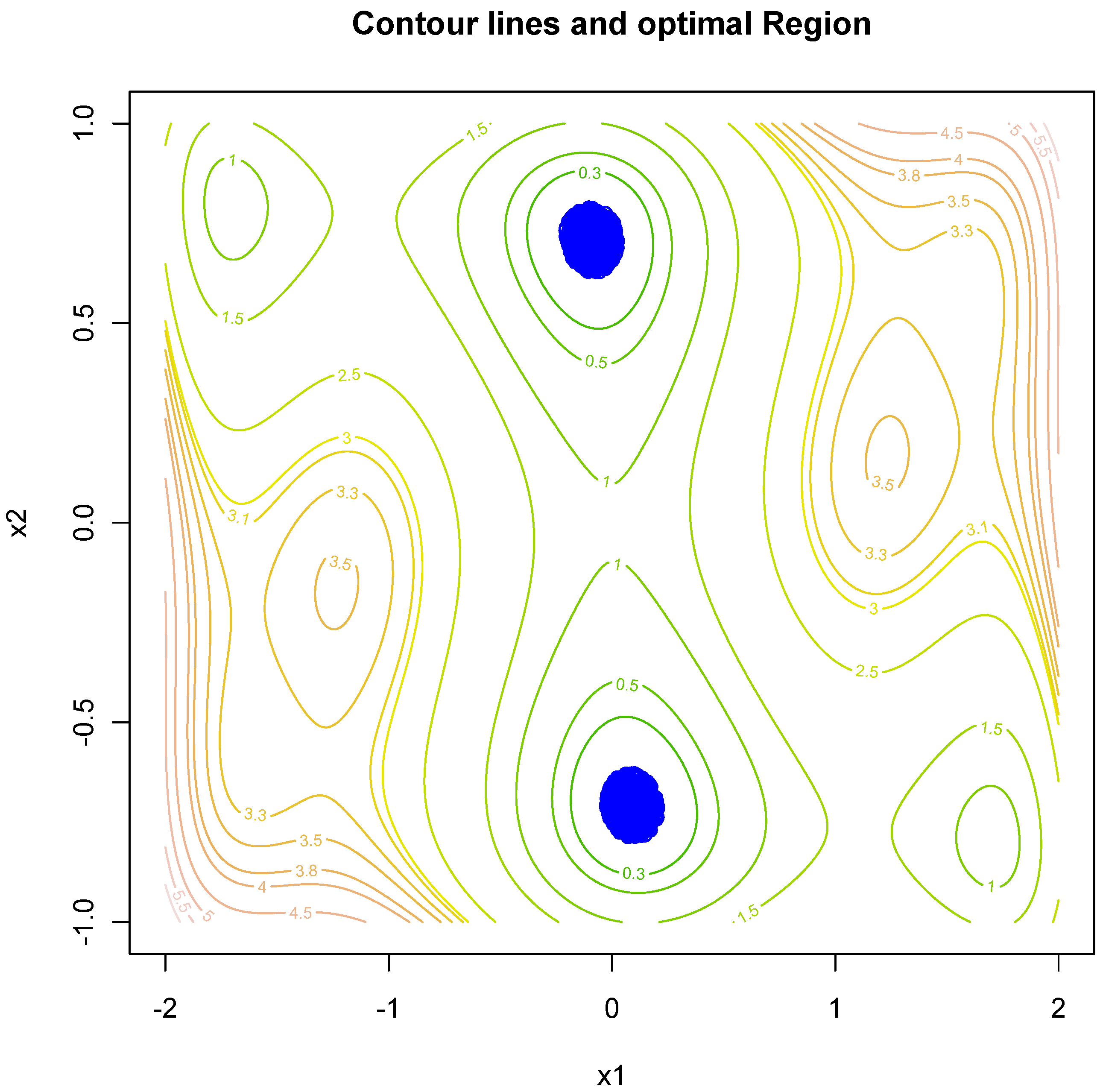

Figure 7.
Study area: Upper Neckar catchment in southwest Germany.
Figure 7.
Study area: Upper Neckar catchment in southwest Germany.
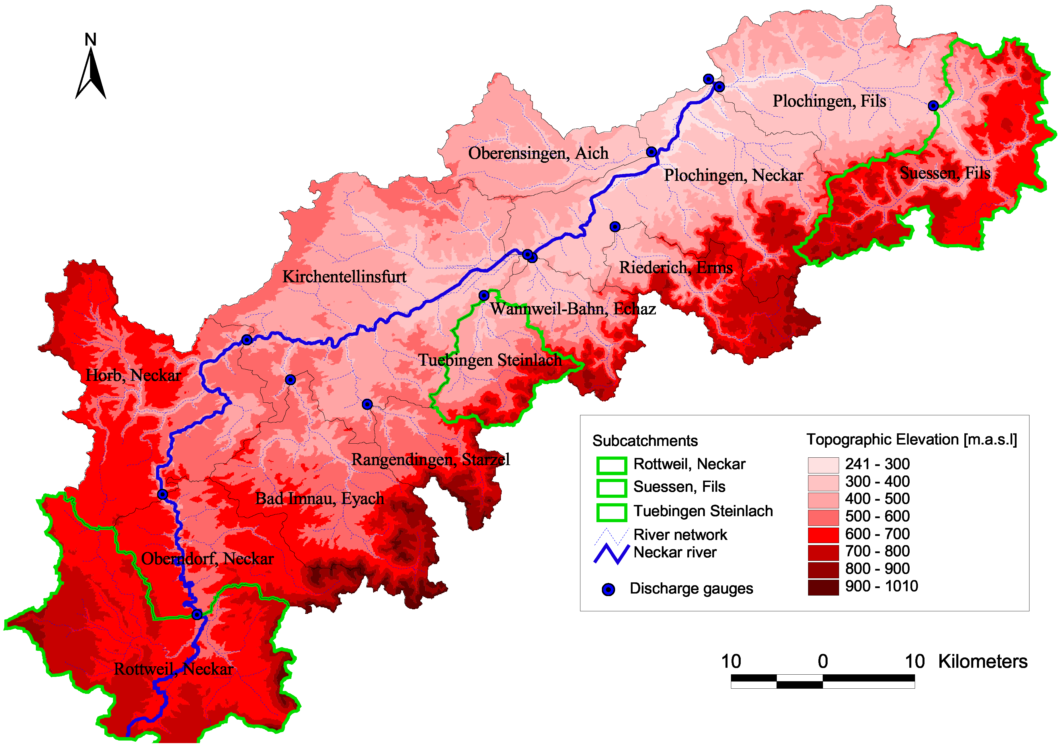
The dataset used in this study includes measurements of daily precipitation from 151 gauges and daily air temperature at 74 climatic stations. The meteorological inputs required for the hydrological model were interpolated from the observations with external drift kriging [29] using topographical elevation as the external drift. The mean annual precipitation is 908 mm/year. Land use is mainly agricultural in the lowlands and forest in the medium elevation ranges. The hydrological characteristics of the three selected sub-catchments are given in Table 6. Table 7 contains runoff and precipitation characteristic for different time periods. For further details, please refer to Samaniego [30, Bárdossy et al. [31] and Singh [19].
Table 6.
Summary of the catchment characteristics of the different sub-catchments in the study area.
| Sub-catchment | Sub-catchment | Elevation | Slope | Mean Discharge | Annual | |
|---|---|---|---|---|---|---|
| size (km2) | (m) | (degrees) | (m3/s) | Precipitation (mm) | ||
| 1 | Rottweil | 454.65 | 555–1010 | 0–34.2 | 5.1 | 968.16 |
| () | ||||||
| 2 | Tübingen | 140.21 | 340–880 | 0–38.8 | 1.7 | 849.84 |
| () | ||||||
| 3 | Süssen | 345.74 | 360–860 | 0–49.3 | 5.9 | 1003.45 |
| () |
Table 7.
Runoff characteristics for different time periods for the case study area.
| Sub-catchment | Rottweil (Neckar) | Tübingen (Steinlach) | Süssen (Fils) | |||
|---|---|---|---|---|---|---|
| Time period | Annual | Annual | Annual | Annual | Annual | Annual |
| Precipitation | Discharge | Precipitation | Discharge | Precipitation | Discharge | |
| (mm) | (mm) | (mm) | (mm) | (mm) | (mm) | |
| 1961–1970 | 997.53 | 375.26 | 851.84 | 400.36 | 1007.94 | 575.55 |
| 1971–1980 | 908.48 | 309.36 | 808.14 | 366.62 | 960.02 | 512.62 |
| 1981–1990 | 997.21 | 385.66 | 888.84 | 404.86 | 1041.72 | 541.81 |
3.3. HYMOD Model
A modified version of the conceptual HYMOD model has been used for this study. HYMOD is a simple conceptual model. This model has two main components, namely rainfall excess (two parameters) and two series of linear reservoirs (three parameters, three identical quick and single for the slow response) in parallel as routing components. The model is based on the characteristics of the runoff production process at a point in a catchment, and then, a probability distribution, which describes the spatial variation in the catchments, is derived by an algebraic expression [32]. This model makes an assumption that the soil structure, texture and water storage capacity vary across the catchment. Therefore, the distribution function of different storage capacities is described as:

Figure 8.
Schematic representation of the hydrological model (HYMOD) model.
Figure 8.
Schematic representation of the hydrological model (HYMOD) model.
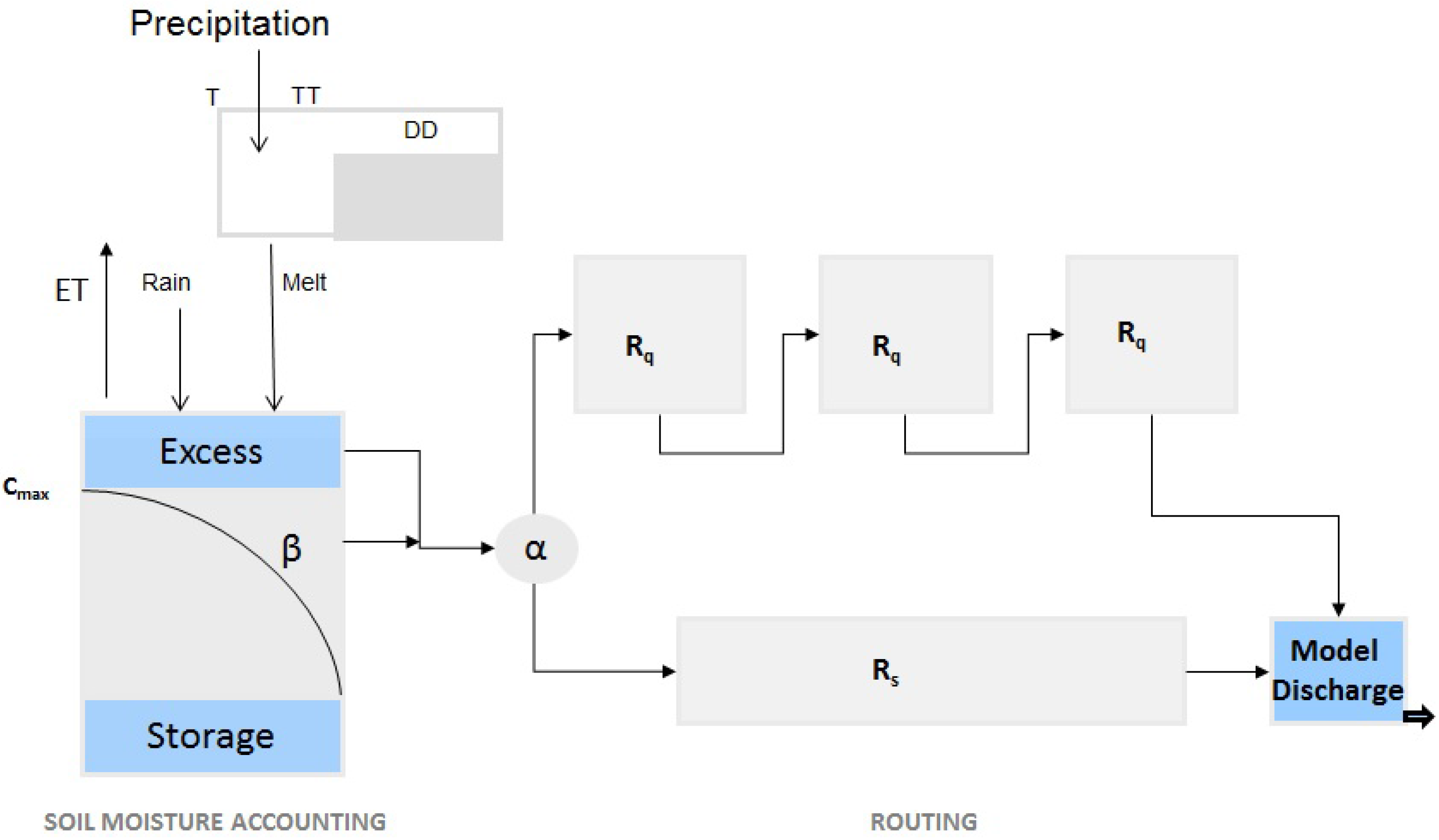
The model structure is shown in Figure 8. The modified HYMOD has eight parameters to conceptualize the hydrological process of the water cycle. The five parameters of this model are the maximum storage capacity in the catchment (), the degree of spatial variability of the soil moisture capacity within the catchment (β), the factor distributing the flow between the two series of reservoirs (α) and the residence times of the linear reservoirs ( and ). The modification in HYMOD was done by adding snow routine. The snow accumulation or melting is calculated based on the degree day method. The three model parameters related to snow are the threshold temperature for snow melt initiation (), degree-day factor () and precipitation/degree-day relation (). Additional information about the HYMOD model in general can be found in Moore [32], Wagener et al. [33], Boyle et al. [34].
4. Result and Discussion
The SRWP algorithm has consistently performed well for all of the simple to complex theoretical test functions. Hence, it was further tested on a hydrological model. All eight parameters of the HYMOD model were calibrated for the time period 1961–1970 by the above-mentioned method and validated for other time periods (1971–1980, 1981–1990 and 1991–2000) for all three sub-catchments, respectively. The rainfall-runoff ratio of the three sub-catchments are 0.37, 0.47 and 0.57 for Rottweil (Neckar), Tübingen (Steinlach) and Süssen (Fils), respectively. The catchments area varies from 140 to 454 km2 for the three sub-catchments; irrespective of the different catchment behaviors, the calibration and validation results from all of the sub-catchments were similar. This may be due to the general feature (non-catchment dependent) of the proposed methodology. Hence, results from only one sub-catchment (Rottweil) are discussed here. Any objective function can be used in the SRWP algorithm. In this study, the most commonly used Nash–Sutcliffe coefficient [35] was used for the evaluation of model performance. Figure 9 shows the stepwise improvement of performance due to sequential replacement of weak parameters with deeper and good parameter sets. It can be seen from Figure 9 that the mean Nash–Sutcliffe coefficient (NS) has improved from 0.64 to 0.69 (as more and more weak parameter sets were replaced with good and deeper parameter sets). There is a gradual improvement in maximum NS, as well. It could be improved further if we allow for more iterations, but it will make the parameter space further shrink and, thus, reduce the transferability and robustness of the parameter space. If more iterations are to be carried out, it would eventually converge to a best single parameter set, which is not necessarily the best for other time periods and can be sensitive, too. Therefore, it is a trade-off to keep the space large enough to be robust and transferable. It can be seen from the same figure that the difference of the maximum and minimum decreases to a point acceptable for the purposes of the modeling exercise. This result shows that after a certain number of replacements of parameters, we cannot get much improvement in the model performance, so we can stop searching for better parameters. The rate of replacement of weak parameter sets decreases as the number of iterations increases. This is because the volume of the parameter space shrinks so much that there is very little scope to improve the model parameters. It is very obvious that when our criteria of difference between maximum and minimum performance is less, we need more iterations and need more parameter replacements. Optimal parameters after the calibration were transferred to different validation time periods to test the transferability of the optimal parameters over time. Table 8 shows the calibration results using the SRWP and transferability of the parameters to validation time periods (1971–1980, 1981–1990 and 1991–2000). The maximum and minimum NS varies between 0.7 and 0.68 with a mean of 0.69. This small variation of maximum and minimum within the optimal parameter space shows that any small change in parameters will not effect the performance. An example of the observed and model hydrograph for the calibration time period is given in Figure 10. The model hydrograph is reasonably well represented for low- to medium-range flooding, but it has missed the very high peaks. We believe this is mainly under-representation of precipitation in the catchment. The calibrated model parameters were tested on validation time periods. The mean NS varies from 0.63–0.75 for different validation time periods. For the period 1981–1990, mean NS is the highest among the other time periods. It is very clear that the parameters have performed well for all three time periods. This shows that the parameters obtained during the calibration by the SRWP algorithm are hydrologically reasonable and transferable. An example of the observed and model hydrographs for the validation time period (1970–1980) is given in Figure 11. The model hydrograph is reasonably well represented for low- to medium-range floods, but it has been over-predicted for some of the floods.
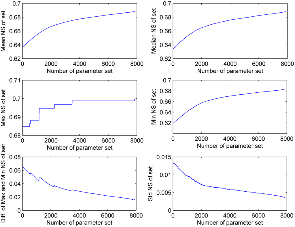
Figure 9.
Improvement of the model performance curve in terms of the Nash–Sutcliffe coefficient (NS) during the calibration by the SRWP algorithm for Rottweil catchment (Diff. is difference; std.is the standard deviation). ROPE, robust parameter estimation; SCE-UA, shuffled complex evolution-University of Arizona.
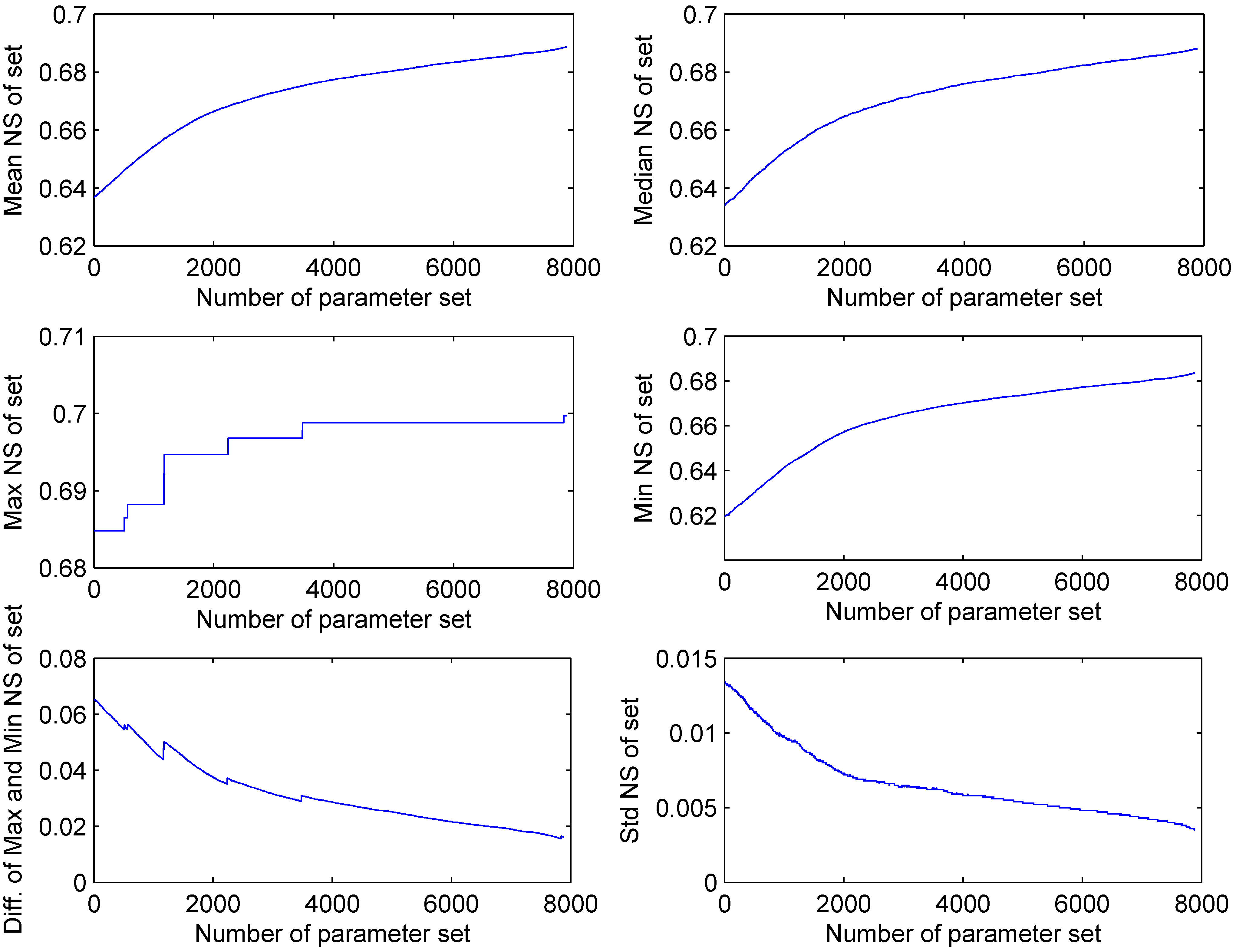
Table 8.
Model performance for calibration time period 1961–1970 and validation for other time periods for Rottweil using the SRWP, ROPE and SCE-UA algorithms (the statistics of 1000 parameter sets are given for the SRWP and ROPE algorithms).
| SRWP | ROPE | SCE-UA | |||||||
|---|---|---|---|---|---|---|---|---|---|
| Periods | mean | max | min | std | mean | max | min | std | |
| 1961–1970 | 0.69 | 0.70 | 0.68 | 0.0035 | 0.69 | 0.70 | 0.69 | 0.0017 | 0.70 |
| 1971–1980 | 0.63 | 0.65 | 0.56 | 0.0135 | 0.63 | 0.64 | 0.58 | 0.0090 | 0.64 |
| 1981–1990 | 0.75 | 0.76 | 0.71 | 0.0082 | 0.75 | 0.76 | 0.72 | 0.0062 | 0.74 |
| 1991–2000 | 0.68 | 0.70 | 0.64 | 0.0104 | 0.68 | 0.70 | 0.65 | 0.0086 | 0.69 |
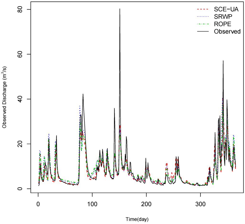
Figure 10.
Example of the observed and model hydrographs during the calibration period from the ROPE, SRWP and SCE-UA algorithms for Rottweil catchment.
Figure 10.
Example of the observed and model hydrographs during the calibration period from the ROPE, SRWP and SCE-UA algorithms for Rottweil catchment.
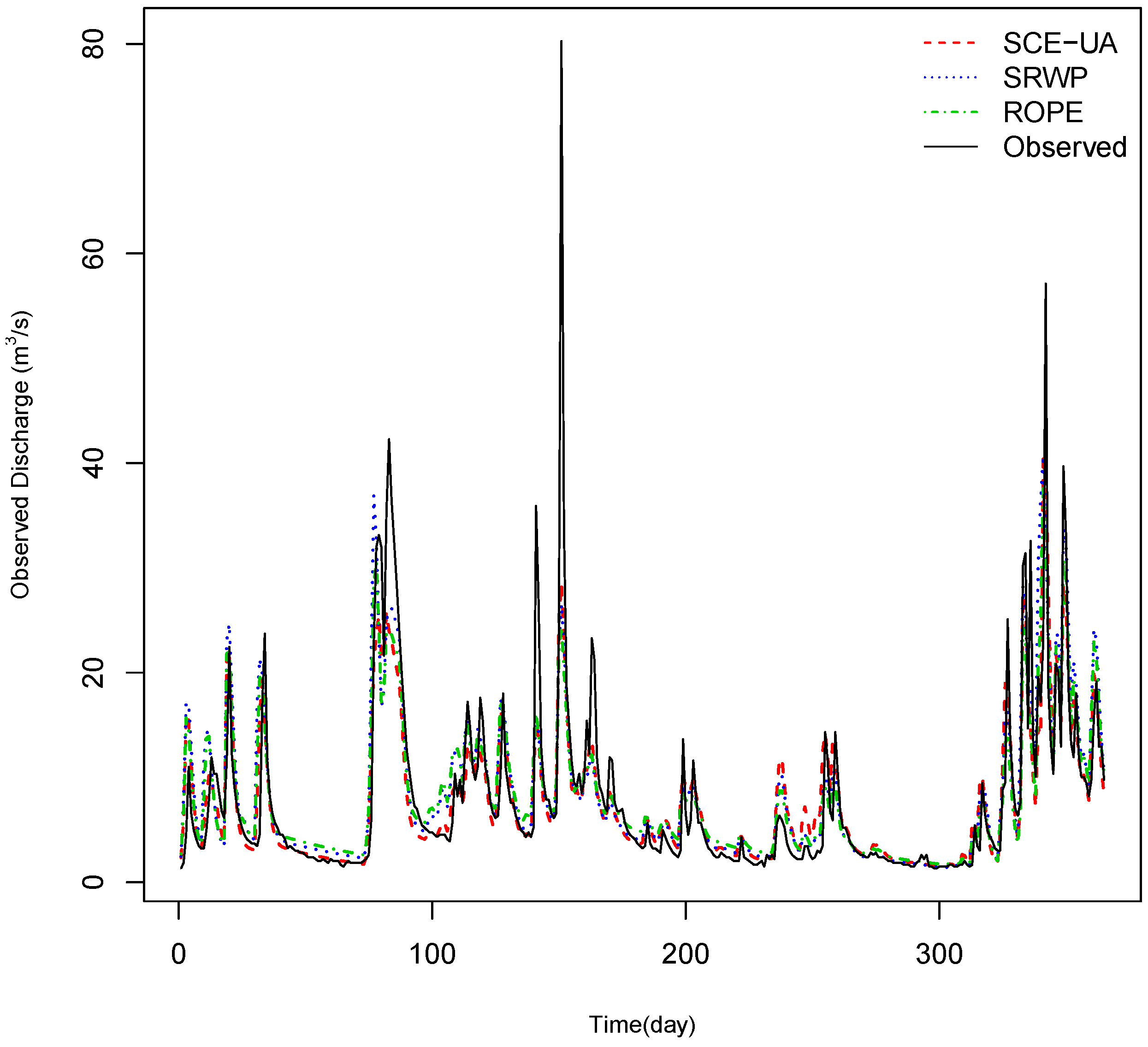
Table Table 9 shows the initial and final range of parameters of the model. It is clear from the table that we have a wide range of parameters after the calibration. Though the volume of the optimal parameter space has shrunk, the range of parameter values remains large with respect to the initial parameter range. This gives flexibility in choosing parameters, where a small change in parameters will not bring much effect in performance. Figure 12 showed the spread of the parameter range at the initial N percentage to the final parameters sets. It can be seen from the figure that at the N percentage, we have a wide range of parameters, which have narrowed down as the number of iterations increased. As we cannot plot an eight-dimensional figure, hence a plot matrix is made for clear visualization. Figure 13 shows the plot matrix of the initial N percentage parameters. It can be seen from the figure that there is no clear structure of any parameters. However, from the final plot matrix of the parameter (Figure 14), we can see that the parameter vector has less scatter and more structure. This is because the volume of the parameter space has shrunk as the number of iterations increased.
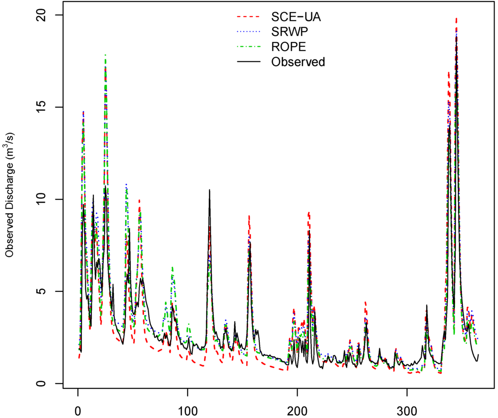
Figure 11.
Example of the observed and model hydrographs during the validation period (1971–1980) from the ROPE, SRWP and SCE-UA algorithms for Rottweil catchment.
Figure 11.
Example of the observed and model hydrographs during the validation period (1971–1980) from the ROPE, SRWP and SCE-UA algorithms for Rottweil catchment.

Table 9.
Initial and final model parameter range obtained during calibration by the SRWP algorithm and calibration by the SCE-UA algorithm for Rottweil catchment.
| Parameters | Initial | SRWP | ROPE | SCE-UA | |
|---|---|---|---|---|---|
| Cmax | Max | 600.0 | 564.02 | 573.67 | 258.58 |
| min | 150.0 | 230.18 | 294.68 | ||
| Beta | Max | 8.0 | 7.34 | 6.91 | 6.01 |
| min | 3.0 | 3.36 | 3.73 | ||
| Alpha | Max | 0.8 | 0.55 | 0.53 | 0.53 |
| min | 0.2 | 0.37 | 3.73 | ||
| Max | 0.2 | 0.02 | 0.02 | 0.02 | |
| min | 0.01 | 0.01 | 0.01 | ||
| Max | 0.7 | 0.68 | 0.68 | 0.65 | |
| min | 0.3 | 0.59 | 0.59 | ||
| Th | Max | 1.5 | 1.40 | 1.10 | 0.78 |
| min | −1.0 | 0.19 | 0.28 | ||
| DD | Max | 3.0 | 2.90 | 2.87 | 2.27 |
| min | 1.0 | 1.17 | 1.39 | ||
| Dew | Max | 2.0 | 0.90 | 1.68 | 0.22 |
| min | 0.0 | 0.08 | 0.09 |

Figure 12.
Model parameters at different stages of the SRWP algorithm (the y-axis is the normalized parameter value, and the x-axis shows all of the parameters of the HYMOD model).
Figure 12.
Model parameters at different stages of the SRWP algorithm (the y-axis is the normalized parameter value, and the x-axis shows all of the parameters of the HYMOD model).
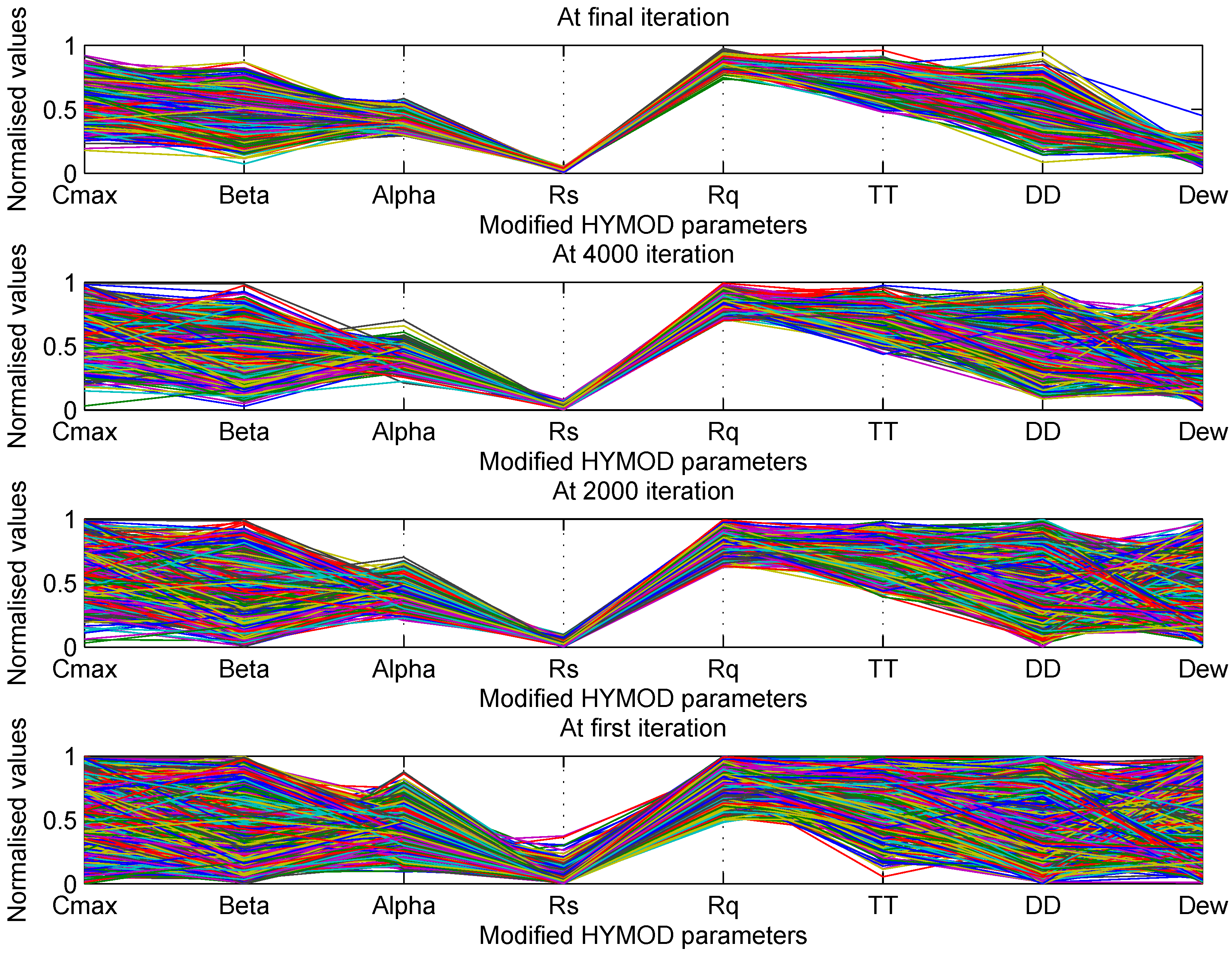
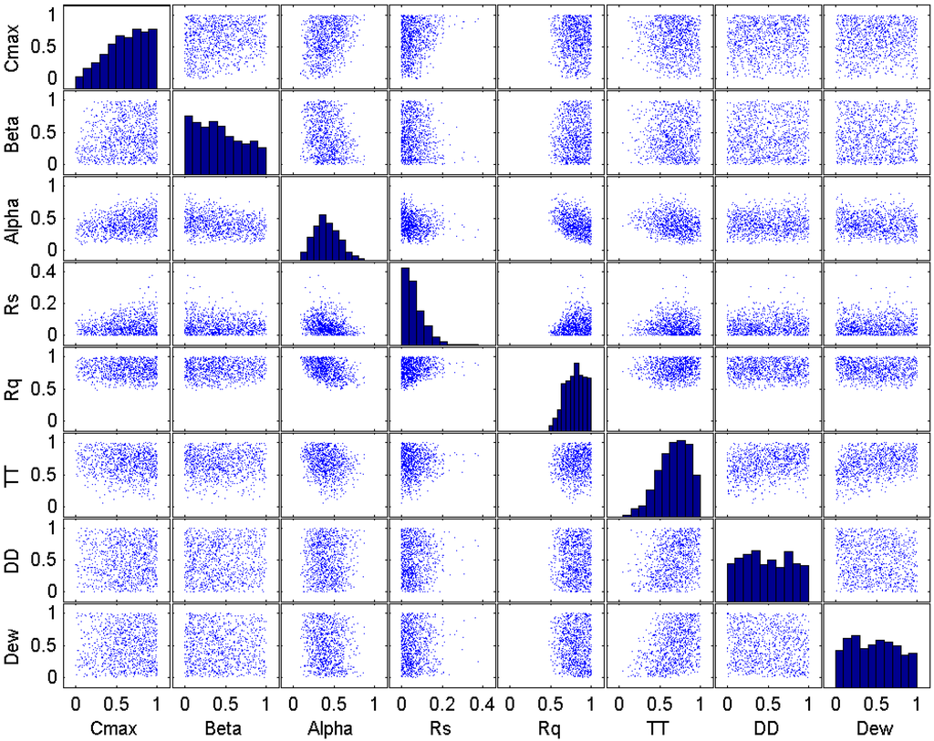
Figure 13.
Plot matrix of the model parameter at the initial iteration of the SRWP algorithm.
Figure 13.
Plot matrix of the model parameter at the initial iteration of the SRWP algorithm.
Figure 14.
Plot matrix of the parameter at the final iteration of the SRWP algorithm.
Figure 14.
Plot matrix of the parameter at the final iteration of the SRWP algorithm.
4.1. Comparison with Existing Methods
The SRWP algorithm is an extension of the ROPE algorithm. Hence, the result obtained by the SRWP algorithm was compared with the previous study by Bárdossy and Singh [5] on the same study area using the ROPE algorithm. The performance of the HYMOD model during the calibration and validation time period obtained by the ROPE algorithm on Rottweil catchment is given in Table 8. It can be seen from Table 8 that the performance by both of the methods is very similar for both the calibration and validation time periods; however, SRWP requires fewer iterations to achieve an optimal parameter space when compared to ROPE (8000 vs. 30,000 parameter evaluations). The robustness of the ROPE algorithm is still maintained by the sequential calibration method, as both use the data depth function to generate new parameters. For further comparison, the HYMOD model was calibrated using the commonly-used global optimization algorithm SCE-UA [27]. Table 8 shows the calibration and validation performance of the HYMOD model using SCE-UA for Rottweil catchment. It can be seen clearly from Table 8 that the calibration of the model using the methodology developed in this paper has very similar results when compared to global optimization with SCE-UA. The validation performance for all three time periods was very much similar to the mean performance obtained by the SRWP algorithm. Very similar results from all three optimization algorithms indicate that the model is well calibrated. Any additional effort to parameterize the model may lead to over-parameterization. Irrespective of the optimization algorithm, the performance of any given model is limited by uncertainty in inputs, parameter estimation, model structure, etc. The hydrographs obtained by ROPE, SRWP and SCE-UA calibration for the calibration and validation time periods are given in Figure 10 and Figure 11. From these figures, we can see that the hydrographs obtained by all three (ROPE, SRWP, SCE-UA) are reasonably good for low to medium high flow, but all of them have missed very high flow in the calibration period. During the validation, SCE-UA is slightly under predicting the low flow and over estimating the high flow, compared to SRWP and ROPE. The final parameters obtained by SCE-UA optimization are given in Table 9. These parameters are a subset of the optimal parameter range obtained by the SRWP algorithm. The result of the sequential calibration method is better compared to SCE-UA and ROPE, due to its robustness in the transferability of parameters in time and quick convergence. Furthermore, it does not depend on the initial values, as initial runs of SRWP start with a wide range of parameters. The advantage of the SRWP calibration method over global optimization can be explained from the final parameter sets. In the SRWP calibration method, we get a parameter space instead of a single value of the parameter set. The single optimal parameter set indeed is a subset of the optimal parameter space. Within the optimal parameter space, small changes in the parameters set do not affect the model performance. For prediction purposes, the deepest parameter set in the convex hull of the optimal space can be used, as well as an ensemble of parameter sets can be drawn from the optimal parameter space, which can account for the parameter uncertainty. Over fitting can be avoided by SRWP, as it always replaces the weak parameters with better parameters, while still maintaining the optimal space. The major limitation of the SRWP algorithm is, after many iterations, when the parameter space is small, it takes more time to get new acceptable parameters. Defining a wider range of parameters for initial runs can be the limitation of SRWP-based calibration.
5. Conclusion
This current work is an advancement of our previous work on the ROPE algorithm [5]. The major improvement of the ROPE algorithm by the sequential replacement of weak parameters algorithm can be seen in terms of convergence efficiency. In sequential replacements of weak parameter sets, we can convergefaster than the ROPE algorithm, as each time, we are replacing weaker model parameters by deeper and good parameter sets sequentially. The other properties, like transferability to other time periods and sensitivity of parameters, remain the same in the sequential replacement of weak parameters algorithm. The result of the SRWP calibration method is comparable to the commonly-used global optimization technique (SCE-UA). The biggest advantage is that it converges to the optimal parameter space, and we can use any kind of criteria or objective functions. Further, instead of a single value as the best parameter set, the sequential calibration method gives an optimal parameter space in which numerous sets of parameters can exist. This can help to define uncertainty due to parameter estimation.
The SRWP procedure clearly shows consistent results over the range of the problem tested. The SRWP algorithm is not model dependent and can be easily implemented on any optimization problem, but further studies may be needed to test the algorithm on more difficult problems. To test the suitability of the SRWP algorithm for very complex multimodal and very high-dimensional problems, it may need to be tested on composite complex functions, such as those proposed by Liang et al. [36]. The authors are working towards this.
Acknowledgments
The work described in this paper was supported by a scholarship program initiated by the German Federal Ministry of Education and Research (BMBF) under the program of the International Postgraduate Studies in Water Technologies (IPSWaT) for the first author. Its contents are solely the responsibility of the authors and do not necessarily represent the official position or policy of the German Federal Ministry of Education and Research and the other organizations to which the other authors belong. The authors would like to thank Guoshui Lui (editor) and three anonymous reviewers for valuable comments and suggestions, which greatly enhanced the quality of the manuscript. The authors would also like to thank Scott Graham for the English editing.
Author Contributions
Both of the authors have made equal contributions in this research.
Conflicts of Interest
The authors declare no conflict of interest.
Appendix A
Some of the test functions used in this study are given below. For more details, please refer to [27] and [28].
A.1. McCormick Function
Search domain: and
A.2. Levy Function
Search domain: and
A.3. Styblinski–Tang Function
Search domain: and
A.4. Leon Function
Search domain: and
A.5. Giunta Function
Search domain: and
A.6. Rastrigin Function
Search domain: and
A.7. Six-Hump Camel Back Function
Search domain: and
References
- Gupta, H.; Sorooshian, S.; Hogue, T.S.; Boyle, D.P. Advances in Automatic Calibration of Watershed Models. In Calibration of Watershed Models; American Geophysical Union: Washington, DC, USA, 2013; pp. 9–28. [Google Scholar]
- Tolson, B.A.; Shoemaker, C.A. Dynamically dimensioned search algorithm for computationally efficient watershed model calibration. Water Resour. Res. 2007. [Google Scholar] [CrossRef]
- Hendrickson, J.D.; Sorooshian, S.; Brazil, L.E. Comparison of Newton-Type and Direct Search Algorithms for Calibration of Conceptual Rainfall-Runoff Models. Water Resour. Res. 1988, 24, 691–700. [Google Scholar] [CrossRef]
- Beven, K. A manifesto for the equifinality thesis. J. Hydrol. 2006, 320, 18–36. [Google Scholar] [CrossRef]
- Bárdossy, A.; Singh, S.K. Robust estimation of hydrological model parameters. Hydrol. Earth Syst. Sci. 2008, 12, 1273–1283. [Google Scholar] [CrossRef]
- Kavetski, D.; Kuczera, G.; Franks, S.W. Calibration of conceptual hydrological models revisited: 1. Overcoming numerical artefacts. J. Hydrol. 2006, 320, 173–186. [Google Scholar]
- Sorooshian, S.; Duan, Q.; Gupta, V.K. Calibration of rainfall-runoff models: Application of global optimization to the Sacramento soil moisture accounting model. Water Resour. Res. 1993, 29, 1185–1194. [Google Scholar] [CrossRef]
- Kuczera, G. Efficient subspace probabilistic parameter optimization for catchment model. Water Resour. Res. 1997, 33, 177–185. [Google Scholar] [CrossRef]
- Gupta, H.; Sorooshian, S.; Yapo, P. Toward improved calibration of hydrologic models: Multiple and noncommensurable measures of information. Water Resour. Res. 1998, 34, 751–763. [Google Scholar] [CrossRef]
- Andréassian, V.; Perrin, C.; Michel, C.; Usart-Sanchez, I.; Lavabre, J. Impact of imperfect rainfall knowledge on the efficiency and the parameters of watershed models. J. Hydrol. 2001, 250, 206–223. [Google Scholar] [CrossRef]
- Beven, K.; Freer, J. Equifinality, data assimilation, and data uncertainty estimation in mechanistic modelling of complex environmental systems using the GLUE methodology. J. Hydrol. 2001, 249, 11–29. [Google Scholar] [CrossRef]
- Vrugt, J.A.; Bouten, W.; Gupta, H.V.; Sorooshian, S. Toward improved identifiability of hydrologic model parameters: The information content of experimental data. Water Resour. Res. 2002, 38, 1312. [Google Scholar] [CrossRef]
- Wagener, T.; McIntyre, N.; Lees, M.J.; Wheater, H.S.; Gupta, H.V. Towards reduced uncertainty in conceptual rainfall-runoff modelling: Dynamic identifiability analysis. Hydrol. Process. 2003, 17, 455–476. [Google Scholar] [CrossRef]
- Samaniego, L.; Bárdossy, A. Robust parametric models of runoff characteristics at the mesoscale. J. Hydrol. 2005, 303, 136–151. [Google Scholar] [CrossRef]
- Kavetski, D.; Kuczera, G.; Franks, S. Calibration of conceptual hydrological models revisited: 2. Improving optimization and analysis. J. Hydrol. 2006, 320, 187–201. [Google Scholar]
- Bárdossy, A. Calibration of hydrological model parameters for ungauged catchments. Hydrol. Earth Syst. Sci. 2007, 11, 703–710. [Google Scholar] [CrossRef]
- Tukey, J. Mathematics and picturing data. In Proceedings of the 1975 International 17 Congress of Mathematics, Vancouver, BC, Canada, 21–29 August 1975; Volume 2, pp. 523–531.
- Singh, S.K.; Bárdossy, A. Calibration of Hydrological Models on Hydrologically Unusual Events. Adv. Water Resour. 2011. [Google Scholar] [CrossRef]
- Singh, S.K. Robust Parameter Estimation in Gauged and Ungauged Basins. Ph.D. Thesis, University of Stuttgart, Stuttgart, BW, Germany, 2010. [Google Scholar]
- Rousseeuw, P.J.; Struyf, A. Computing location depth and regression depth in higher dimensions. Stat. Comput. 1998, 8, 193–203. [Google Scholar] [CrossRef]
- Liu, R.Y.; Parelius, J.M.; Singh, K. Multivariate analysis by data depth: Descriptive statistics, graphics and inference. Ann. Stat. 1999, 27, 783–858. [Google Scholar]
- Zuo, Y.; Serfling, R. General notions of statistical depth function. Ann. Stat. 2000, 28, 461–482. [Google Scholar] [CrossRef]
- Chebana, F.; Ouarda, T.B.M.J. Depth and homogeneity in regional flood frequency analysis. Water Resour. Res. 2008. [Google Scholar] [CrossRef]
- Dutta, S.; Ghosh, A.K.; Chaudhuri, P. Some intriguing properties of Tukey’s half-space depth. Bernoulli 2011, 17, 1420–1434. [Google Scholar] [CrossRef]
- Singh, S.K.; McMillan, H.; Bárdossy, A. Use of the data depth function to differentiate between case of interpolation and extrapolation in hydrological model prediction. J. Hydrol. 2013, 477, 213–228. [Google Scholar] [CrossRef]
- Singh, S.K.; Jain, S.K.; Bárdossy, A. Training of artificial neural networks using information-rich data. Hydrology 2014, 1, 40–62. [Google Scholar] [CrossRef]
- Duan, Q.; Gupta, V.; Sorooshian, S. Shuffled complex evolution approach for effective and efficient global minimization. J. Optim. Theory Appl. 1993, 76, 501–521. [Google Scholar] [CrossRef]
- Mishra, S.K. Some new test functions for global optimization and performance of repulsive particle swarm method. 2006. MPRA Paper No. 2718, posted 07. Available online: http://mpra.ub.uni-muenchen.de/2718/ (accessed on 22 April 2015).
- Ahmed, S.; de Marsily, G. Comparison of geostatistical methods for estimating transmissivity using data transmissivity and specific capacity. Water Resour. Res. 1987, 23, 1717–1737. [Google Scholar] [CrossRef]
- Samaniego, L. Hydrological Consequences of Land Use/Land Cover Change in Mesoscale Catchments. Transactions of the Institute of Hydraulic Engineering. Ph.D. Thesis, University of Stuttgart, Stuttgart, Germany, 2003. [Google Scholar]
- Bárdossy, A.; Pegram, G.S.; Samaniego, L. Modeling data relationships with a local variance reducing technique: Applications in hydrology. Water Resour. Res. 2005. [Google Scholar] [CrossRef]
- Moore, R.J. The probability-distributed principle and runoff production at point and basin scales. Hydrol. Sci. J. 1985, 30, 273–297. [Google Scholar] [CrossRef]
- Wagener, T.; Boyle, D.P.; Lees, M.J.; Wheater, H.S.; Gupta, H.V.; Sorooshian, S. A framework for development and application of hydrological models. Hydrol. Earth Syst. Sci. 2001, 5, 13–26. [Google Scholar] [CrossRef]
- Boyle, D.P.; Gupta, H.V.; Sorooshian, S.; Koren, V.; Zhang, Z.; Smith, M. Toward Improved Streamflow Forecasts: Value of Semidistributed Modeling. Water Resour. Res. 2001, 37, 2749–2759. [Google Scholar] [CrossRef]
- Nash, J.; Sutcliffee, J. River flow forecasting through conceptual models. 1. A discussion of principles. J. Hydrol. 1970, 10, 282–290. [Google Scholar] [CrossRef]
- Liang, J.; Suganthan, P.; Deb, K. Novel composition test functions for numerical global optimization. In Proceedings of the 2005 IEEE, Swarm Intelligence Symposium, SIS, Pasadena, CA, USA, 8–10 June 2005; pp. 68–75.
© 2015 by the authors; licensee MDPI, Basel, Switzerland. This article is an open access article distributed under the terms and conditions of the Creative Commons Attribution license (http://creativecommons.org/licenses/by/4.0/).