Article

Seasonal Inflow Shifts and Increasing Hot–Dry Stress for Eagle Mountain Lake Reservoir, Texas: SWAT Modeling with Downscaled CMIP6 Daily Climate and Observed Operations

1
Department of Environmental & Geological Sciences, Texas Christian University, Fort Worth, TX 76129, USA
2
Department of Environmental Science & Technology, Jashore University of Science & Technology, Jashore 7408, Bangladesh
*
Author to whom correspondence should be addressed.
Hydrology 2026, 13(2), 63; https://doi.org/10.3390/hydrology13020063
Submission received: 6 January 2026 / Revised: 30 January 2026 / Accepted: 3 February 2026 / Published: 6 February 2026

Abstract

Climate change can alter both the amount and timing of inflows to water supply reservoirs while also increasing heat-driven demand and the likelihood of stressful warm-season conditions. Climate-driven changes in inflow to Eagle Mountain Lake Reservoir (Texas, USA) were quantified by integrating (i) a calibrated SWAT model evaluated at four USGS stream gauges, (ii) statistically downscaled CMIP6 daily precipitation and minimum/maximum temperature at seven stations/grid points for a historical baseline (2003–2022) and two future windows (2031–2050 and 2081–2100) under SSP1-2.6, SSP2-4.5, and SSP5-8.5, and (iii) observed reservoir operations (lake level, water supply releases, and flood discharge; 1990–2022). A standard watershed climate workflow is reframed through an operations-focused lens, wherein projected inflow changes are translated into decision-relevant indicators via the utilization of observed thresholds and operating mode signals. Included within this framework are spring refill-season inflow shifts, a hot–dry month metric, and storage threshold performance measures, which are coupled with screening-level probabilities linked to multi-year inflow deficits. Across models and stations, mean annual temperature increases by 0.7–1.9 °C in the 2030s and by 0.7–6.1 °C in the 2080s, while annual precipitation changes remain uncertain (−24% to +55%). Daily projections show a strong increase in extreme heat days (daily Tmax above the historical 95th percentile), from about 18 days yr−1 historically to about 30–33 days yr−1 in the 2030s and about 34–82 days yr−1 by the 2080s. Hot–dry months (monthly mean Tmax above the historical 90th percentile and monthly precipitation below the historical median) increase modestly by mid-century and rise to about 1.5 months yr−1 on average by the 2080s under SSP5-8.5. SWAT simulations indicate that the mean annual inflow declines by 17–20% across scenarios, with the largest reductions during the spring refill period (March–June). Historical operations show that hot–dry months are associated with approximately double the mean water supply release (7.2 vs. 3.5 m3/s) and a lower monthly minimum lake level (about 0.30 m; about 1.0 ft lower on average). Flood discharges occur almost exclusively when lake elevation is at or above about 197.8 m and follow multi-day rainfall clusters (cross-validated AUC = 0.99). Together, these results indicate that earlier-season inflow reductions and more frequent hot–dry stress will tighten the operational margin between refill, summer demand, and flood management, underscoring the need for adaptive drought response triggers and integrated drought–flood planning for the Dallas–Fort Worth region.

1. Introduction

Climate change is altering the hydrologic cycle in ways that challenge reservoir systems designed around historical seasonality and stationarity. Warmer temperatures increase atmospheric demand and evaporative losses, intensifying heavy precipitation and increasing both drought and flood risks within the same watershed [1,2,3]. For water supply reservoirs, the key operational question is not only whether annual inflow changes, but whether seasonal refill timing shifts and whether stressful warm-season conditions become more frequent [4,5,6].
Recent extremes illustrate why these changes matter for water resources operations. Event attribution studies show that anthropogenic warming can increase the intensity of extreme rainfall, thereby worsening flood hazards and stressing flood management infrastructure (e.g., the 2021 Western European floods) [7,8]. Similar attribution evidence exists for the 2022 Pakistan floods [9]. In the United States, the growing frequency and cost of weather and climate disasters highlight the increasing exposure of water systems to compound hazards [10]. In Texas, Hurricane Harvey (2017) produced multi-day rainfall totals exceeding 1500 mm in some locations and caused approximately $125 billion in damages [11,12].
At the other end of the hydrologic spectrum, persistent warm-season water deficits are becoming more consequential for water supply reliability. Multi-year drought crises, such as the 2020–2023 Horn of Africa drought [13] and the 2000–2023 western U.S. megadrought, illustrate how deficits can persist beyond the buffering capacity of storage when inflows remain suppressed for several consecutive years. The west U.S. megadrought is the driest 23-year period in at least 1200 years, and anthropogenic warming has contributed substantially to soil moisture deficits that intensify hydrologic drought impacts [6,14]. For reservoir operations, these conditions are especially challenging when high heat and low rainfall coincide, because such compound periods align with peak water demand, low inflows, and reduced operating margins for storage and releases [4].
Texas is particularly exposed to climate-driven water supply stress because rapid population growth and climate variability converge on a finite reservoir system. The Texas Water Development Board projects that the statewide population will grow from 29 million in 2020 to more than 51 million by 2070, with water demand increasing by about 22% [15]. The Dallas–Fort Worth metropolitan area exceeds 8 million residents and continues to grow rapidly [16], increasing reliance on surface water reservoirs and heightening sensitivity to seasonal inflow variability and multi-year drought.
Observed records already show warming in Texas and increasing precipitation variability, with more intense rainfall events interspersed with longer dry spells [10,17]. Regional assessments project additional warming and increased intensity of extreme precipitation in the remainder of the 21st century [18,19,20]. Together, these trends imply a more challenging operating envelope for reservoirs: greater warm-season demand and evaporation losses, more frequent hot–dry conditions, and episodic floods that must be buffered without compromising supply reliability.
Together, these lines of evidence emphasize that mean changes alone do not capture the operational stressors that matter most: persistence of deficits, seasonality shifts, and extremes at both tails of the distribution. Accordingly, in addition to SWAT-based inflow projections, we include time series diagnostics and threshold-based indicators to connect projected changes to the historical structure of variability and to decision-relevant triggers.
Eagle Mountain Lake, a reservoir in the Upper West Fork Trinity River basin managed by the Tarrant Regional Water District, supplies drinking water to nearly half a million North Texas residents [21]. Despite its strategic role, peer-reviewed evidence linking projected watershed-scale inflow changes to operationally relevant signals in the reservoir record (storage, releases, and flood discharge) remains limited for this system. This gap matters because management decisions are driven by thresholds (e.g., seasonal refill levels and flood release triggers), not only by annual mean changes.
Watershed models, such as the Soil and Water Assessment Tool (SWAT), provide a practical framework for translating climate scenarios into daily streamflow responses and seasonal shifts in inflow [22,23]. However, many climate impact studies stop at changes in hydrologic statistics, while operators need interpretable indicators that map directly to decisions, such as refill-season inflow reliability, drought trigger frequency, and the occurrence of hot–dry months that coincide with high demand. By combining SWAT projections with observed reservoir operations, this study offers a transparent, management-focused interpretation of climate risks without requiring simulation of proprietary operating rules.
This study aims to quantify how projected climate change may alter streamflow entering Eagle Mountain Lake and to translate those changes into operationally relevant risk signals using the historical reservoir record. Specific objectives are to: (i) develop and evaluate a SWAT model for the Upper West Fork Trinity watershed using long-term USGS streamflow observations; (ii) generate station-scale downscaled daily climate inputs from CMIP6 projections under SSP1-2.6, SSP2-4.5, and SSP5-8.5 for a baseline period (2003–2022) and two future windows (2031–2050; 2081–2100); (iii) quantify projected changes in annual, seasonal, and monthly inflow to the reservoir and characterize inter-model uncertainty; (iv) evaluate historical reservoir storage dynamics and threshold-based performance metrics to characterize drought exposure; and (v) link climate stress metrics, including extreme heat days and “hot–dry months”, to observed operations (water supply releases, lake level, and flood discharge) to provide a compound event framing that matches management reality.
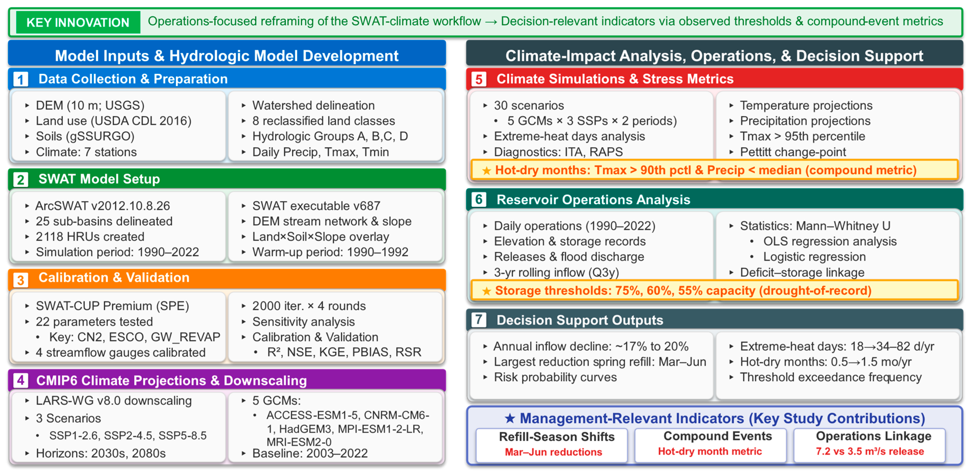
The distinctive contribution of this work is an operational reframing of a standard SWAT-plus-climate workflow. Projected hydroclimatic changes are translated into decision-relevant indicators using the historical operations record: (i) refill-season inflow shifts (March–June), (ii) a hot–dry month metric aligned with warm-season demand, and (iii) storage threshold performance and screening-level probabilities linked to multi-year inflow deficits. This framing is intended to bridge watershed projections and threshold-based reservoir management without requiring simulation of proprietary operating rules.

2. Materials and Methods

For readability, this section is organized into study materials (study area and datasets) and methods (SWAT setup, calibration/validation, CMIP6 downscaling, and statistical/operations analyses). A schematic overview of the end-to-end workflow is provided in Figure 1.

2.1. Study Area

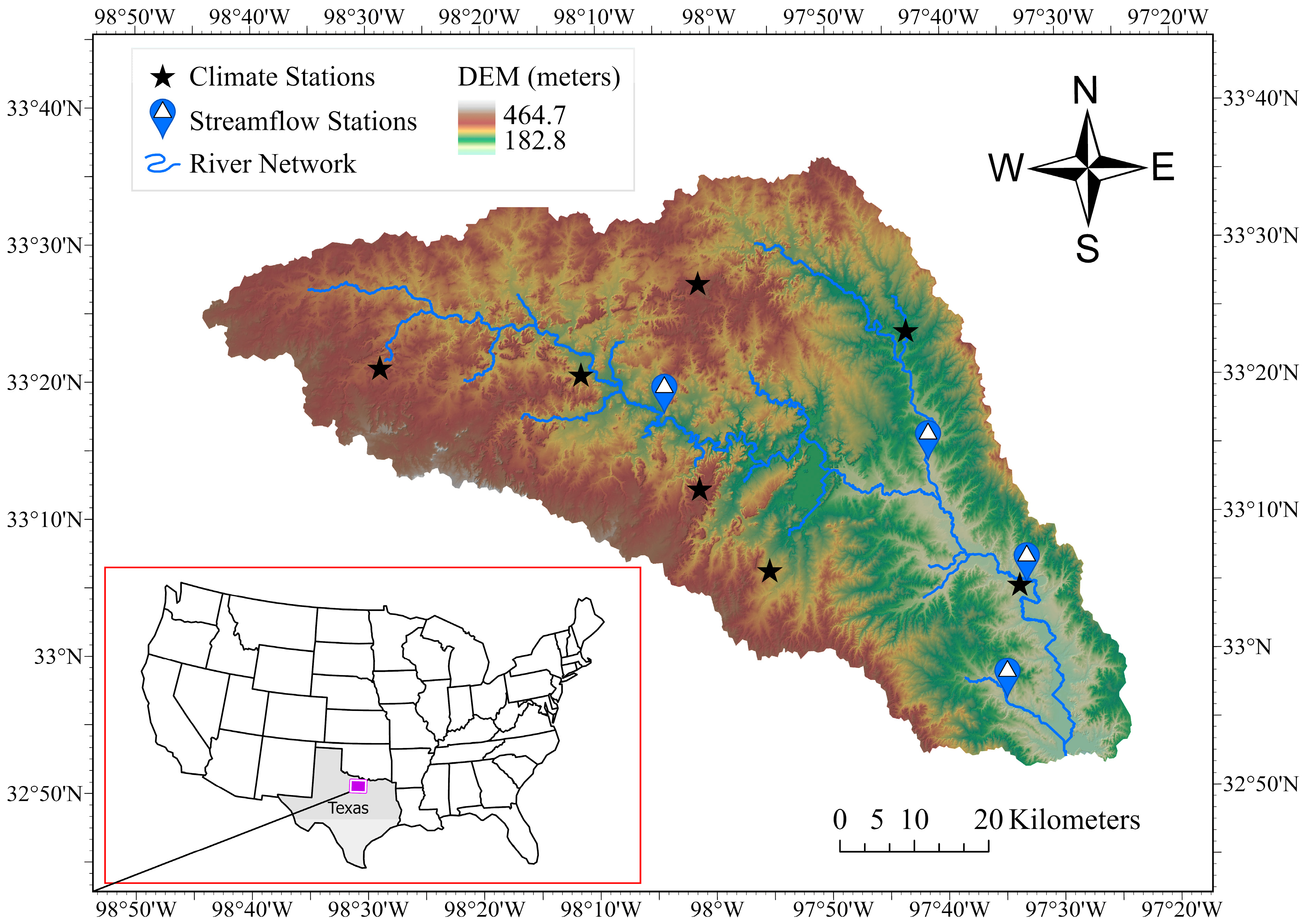
The study focuses on the Eagle Mountain Lake Reservoir watershed in the Upper West Fork Trinity River basin (Hydrologic Unit Code 12030101) in North-Central Texas, USA (Figure 2). Eagle Mountain Lake is located in Tarrant and Wise counties, approximately 8 km (5 mi) northwest of Fort Worth (centered near 32.92° N, 97.50° W) within the Dallas–Fort Worth metropolitan region. The modeled watershed outlet corresponds to the USGS West Fork Trinity River near Boyd gauge (08044500), which drains approximately 4468 km2 upstream of the reservoir. Eagle Mountain Lake has a conservation (normal) storage capacity of approximately 228 million m3 at a conservation pool elevation of about 197.8 m above mean sea level, making it a strategically important component of regional water supply planning.
Land cover in the watershed is dominated by pasture and agricultural lands (65%), followed by forests (18%), urban areas (9%), and other land uses, including water bodies, wetlands, shrublands, and barren land (8%) [24]. The watershed experiences a humid subtropical climate (Köppen–Geiger classification Cfa) characterized by hot summers and mild winters [25]. Based on the seven station records used in this study, mean annual temperature during the baseline period (2003–2022) ranges from 17.8 to 19.0 °C, and mean annual precipitation ranges from 750 to 891 mm. The U.S. Geological Survey (USGS) maintains four active streamflow gauging stations within the watershed, providing discharge measurements for model calibration and validation (Table 1). Eagle Mountain Lake was impounded in 1932. Daily reservoir observations for 1988–2024 indicate that lake surface elevation fluctuated between 194.5 and 200.2 m, and conservation storage ranged from near full pool to approximately 54% during the drought of record [21,26]. In addition to municipal water supply, the reservoir supports recreational activities including fishing, boating, and water sports, generating approximately $1.7 million in annual revenue [21].

2.2. Hydrological Model Description

The Soil and Water Assessment Tool (SWAT) is a physically based, semi-distributed hydrological model developed by the U.S. Department of Agriculture-Agricultural Research Service (USDA-ARS) to simulate the impacts of land management practices on water, sediment, and agricultural chemical yields in large, complex watersheds [22,27]. The SWAT operates on a daily step and divides watersheds into subbasins based on topography, which are further subdivided into Hydrologic Response Units (HRUs), unique combinations of land use, soil type, and slope class that represent homogeneous areas with similar hydrological behavior. The SWAT model simulates the complete terrestrial water cycle, including precipitation, canopy interception, infiltration, evapotranspiration, surface runoff, lateral subsurface flow, groundwater recharge, and channel routing, with the water balance equation governing each HRU.

2.3. Input Data and Model Setup

Model development utilized ArcSWAT version 2012.10.8.26, an ArcGIS 10.8.0 interface compatible with SWAT executable version 687 (swat.tamu.edu). Four primary data layers were required for model construction: (1) topography, (2) land use/land cover, (3) soils, and (4) climate data (Table A1).
A 10 m resolution Digital Elevation Model (DEM) was obtained from the USGS National Elevation Dataset and processed to derive watershed boundaries, stream networks, flow direction, and slope characteristics. Land use/land cover data were obtained from the USDA National Agricultural Statistics Service Cropland Data Layer (2016), which provides 30 m resolution classification based on a modified Anderson Level II system [24]. The original 16 land classes were reclassified into eight broader categories: agricultural land, barren land, forests, urban areas, grass/pasture, wetlands, open water bodies, and shrubland. Soil data were obtained from the USDA Natural Resources Conservation Service (NRCS) gridded Soil Survey Geographic (gSSURGO) database, providing detailed information on soil physical and hydrological properties. Soils were classified into four hydrologic soil groups (A–D) based on infiltration capacity, with Group A representing high-infiltration sandy soils and Group D representing low-infiltration clay soils with high runoff potential (Table A2). Climate data, including daily precipitation and minimum/maximum temperature, were compiled for seven stations/grid points (five stations and two PRISM gridded points) for the period 2003–2022 (Table A3). Station and grid point metadata are retained in the SWAT project input files. Watershed delineation using the 10 m DEM resulted in 25 subbasins. Subsequent HRU delineation, based on unique combinations of land use, soil type, and slope class (<2%, 2–5%, >5%), generated 2118 HRUs. The model was run for the period 1990–2022, with a three-year warm-up period (1990–1992) to allow model state variables to reach equilibrium.

2.4. Model Calibration and Validation

Model calibration and validation were performed using SWAT-CUP Premium [28], employing the SWAT Parameter Estimator (SPE) algorithm with stochastic calibration. Twenty-two parameters controlling surface runoff, baseflow, groundwater, evapotranspiration, and channel routing processes were selected for calibration based on a literature review and preliminary sensitivity analysis (Table A4). A global sensitivity analysis using a multiple regression approach with Latin Hypercube sampling identified the most influential parameters, with significance assessed using t-statistics and p-values. Daily discharge observations from these gauges extend through the calibration/validation period (1990–2022); Table 1 lists the period of record start dates for reference.
Calibration was performed separately for four USGS gauge stations (Table 1) representing different drainage areas and streamflow regimes within the watershed. Watershed, draining to USGS station 08044500 (West Fork Trinity River near Boyd, TX, USA), represents the primary inlet to Eagle Mountain Lake and encompasses 4462 km2 (approximately 80% of the total watershed area). For each USGS gauge, 2000 model iterations were executed across four calibration rounds, with parameter ranges progressively refined based on simulation results.
Model performance was assessed using a suite of five complementary statistical metrics to provide a comprehensive evaluation of the agreement between simulated and observed streamflow: the coefficient of determination (R2), Nash–Sutcliffe Efficiency (NSE), Kling–Gupta Efficiency (KGE), Percent Bias (PBIAS), and the RMSE observations standard deviation ratio (RSR). This multi-metric approach was adopted to capture different aspects of model performance, including correlation, bias, variability, and overall predictive accuracy. NSE was computed as NSE = 1 − [Σ(QobsQsim)2/Σ(QobsQmean)2], where Qobs and Qsim are observed and simulated discharge, and Qmean is the observed mean. KGE was computed as KGE = 1 − [(r − 1)2 + (α − 1)2 + (β − 1)2]1/2, where r is the correlation coefficient, α is the variability ratio (σsim/σobs), and β is the bias ratio (μsim/μobs). PBIAS was computed as PBIAS = 100 × Σ(QsimQobs)/Σ(Qobs), and RSR was computed as RMSE/σobs. For detailed methodological frameworks on SWAT model calibration and uncertainty analysis, readers are referred to Abbaspour et al. [28].

2.5. Future Climate Scenarios

Future climate projections were generated using the Long Ashton Research Station Weather Generator (LARS-WG) version 8.0 [29,30], a stochastic weather generator that produces site-specific daily weather data under both baseline and climate change scenarios. LARS-WG was calibrated using 33 years (1990–2022) of observed daily precipitation and temperature data from each of the seven weather stations in the study area. Model performance was evaluated using chi-square goodness-of-fit tests, t-tests, and F-tests comparing the statistical properties of observed and simulated weather series.
Climate change scenarios were derived from five Global Climate Models (GCMs) participating in the Coupled Model Intercomparison Project Phase 6 (CMIP6): ACCESS-ESM1-5 (Australia), CNRM-CM6-1 (France), HadGEM3-GC31-LL (UK), MPI-ESM1-2-LR (Germany), and MRI-ESM2-0 (Japan) (Table A5). These models were selected because they are implemented within LARS-WG (enabling consistent site-scale statistical downscaling at all seven locations), originate from different modeling centers (providing structural diversity), and span a range of warming rates and hydroclimate responses over North America. We treat the resulting five-model ensemble as a scenario set to bracket uncertainty rather than a probabilistic forecast; therefore, results are reported as ensemble summaries (means and uncertainty ranges) consistent with known inter-model spread in CMIP6 precipitation projections and model sensitivity differences [31,32]. Projections were obtained for three Shared Socioeconomic Pathways: SSP1-2.6 (sustainable development, low emissions), SSP2-4.5 (middle-of-the-road development, moderate emissions), and SSP5-8.5 (fossil-fueled development, high emissions), representing radiative forcing of 2.6, 4.5, and 8.5 W/m2 by 2100, respectively [33,34]. Downscaled daily series were generated for each of the seven station/grid point locations used in this study (Table A3).
Daily climate time series used to force the SWAT and to compute climate metrics were assembled for seven stations within the study area (Alvord, Boyd, Bridgeport, Markley, Newport, PRISM1, PRISM2). The historical baseline spans 2003–2022 and includes daily precipitation and minimum/maximum temperature. Future daily series were developed for two windows, 2031–2050 (2030s) and 2081–2100 (2080s), for five CMIP6 GCMs (Table A5) under SSP1-2.6, SSP2-4.5, and SSP5-8.5. These daily series were used both to drive SWAT simulations and to quantify changes in mean climate, extremes, and management-relevant compound conditions.
Management-relevant climate stress metrics were computed from the downscaled daily series and applied consistently across historical and future periods. Extreme heat days were defined as days with Tmax exceeding the station-specific 95th percentile of the baseline (2003–2022). Hot–dry months were defined as months with a monthly mean Tmax exceeding the station-specific 90th percentile of the baseline and monthly precipitation below the baseline median. Percentile-based temperature thresholds normalize for spatial differences among stations/grid points and identify unusually hot months that remain frequent enough to be operationally meaningful, while the median precipitation threshold provides a robust separator of below-normal rainfall months given precipitation skewness. The combined hot–dry criterion captures periods when atmospheric demand (and typically warm-season water demand) is high while rainfall–runoff generation is suppressed, aligning with conditions that historically coincide with storage drawdown and higher water supply releases.

2.6. Statistical Analysis and Uncertainty Characterization

Streamflow change was quantified at annual, seasonal, and monthly scales using ensemble summaries across five GCMs. Annual and monthly distributions are reported using the mean, median, coefficient of variation (CV), and the 5th–95th percentile range (Q5–Q95). Percent changes were computed relative to the baseline mean (2003–2022).
To interpret climate projections in operational terms, we quantified the climate stress metrics defined above and summarized them alongside streamflow projections. For reservoir operations, differences between hot–dry months and other months were tested using Mann–Whitney U tests, and simple regression and classification models were evaluated using standard metrics (R2 for linear models; AUC and Brier score for flood event classification).

2.7. Time Series Diagnostics of Historical Climate Inputs and Storage

The historical climate input series and the observed storage record were evaluated for trend structure, homogeneity, and multi-year fluctuations using two complementary visualization-based techniques: innovative trend analysis (ITA) [35] and rescaled adjusted partial sums (RAPS) [36]. The goal is not to replace the core SWAT and downscaled climate analyses, but to provide additional context on how the historical record partitions into sub-periods and to confirm that a single step change does not dominate the baseline input data.
ITA was applied to annual basin-average precipitation totals and annual mean temperature derived from the seven-station baseline daily series (2003–2022). Following Sen [35], the annual series was split into two equal sub-periods (2003–2012 and 2013–2022), each sub-series was ranked, and values were plotted against one another relative to the 1:1 line. Points consistently above (below) the 1:1 line indicate an increasing (decreasing) tendency across the distribution. To supplement the ITA visualization, time series homogeneity was also evaluated using the Pettitt nonparametric change point test [37] applied to the annual series. RAPS was applied to the observed monthly conservation storage (% full) record (1988–2024) of the Eagle Mountain Lake Reservoir. RAPS values were computed as the cumulative sum of deviations from the long-term mean, rescaled by the standard deviation, which highlights persistent departures and potential shifts in the mean state.

2.8. Reservoir Observation Analysis

Daily reservoir operations data were compiled for Eagle Mountain Lake from January 1990 to January 2022. The dataset includes (i) lake surface elevation (m), (ii) water supply release rate (m3/s), and (iii) flood discharge (m3/s; release/spill). The operations time series complements the conservation storage record used elsewhere in this study by providing direct information on release behavior and lake level dynamics.
For statistical analysis, reservoir operation variables were aggregated to monthly metrics: mean water supply release, number of flood discharge days, total flood discharge, mean elevation, and monthly minimum elevation. These monthly metrics were merged with basin-average monthly temperature and precipitation derived from the seven-station historical daily climate series for the overlapping period (2003–2021).
To quantify climate–operations linkages without assuming a particular operating policy model, two complementary approaches were used. Firstly, reservoir operation metrics in hot–dry months were compared with those in all other months using nonparametric tests. Secondly, for the demand season (May–September), an ordinary least squares model of monthly mean water supply release as a function of monthly mean Tmax and monthly precipitation was fitted. For flood operations, the daily occurrence of flood discharge (>0) was modeled using logistic regression with predictors representing multi-day precipitation totals and lake elevation; predictive skill was evaluated using time series cross-validation (AUC and Brier score).

2.9. Linking Projected Inflows to Reservoir Operations and Compound Event Screening

Reservoir operations respond to both seasonal timing and persistence of wet and dry conditions, rather than to annual totals alone. To translate SWAT inflow projections into management-relevant risk indicators using available observations, (i) threshold-based performance metrics from the historical conservation storage record and (ii) a screening-level storage risk relationship based on multi-year inflow deficits were combined.
Annual inflow at the reservoir inlet was extracted from SWAT for the baseline period (2003–2022) and for each future GCM-SSP time horizon simulation. To represent multi-year drought persistence, a 3-year rolling mean inflow anomaly (Q3y) was computed. A 3-year window was selected as a compromise between capturing persistence and retaining an adequate sample size for fitting. Sensitivity checks using 2-year and 5-year rolling means produced the same monotonic relationship between sustained inflow deficits and annual minimum lake level, with only modest differences in correlation strength (r increasing from about 0.43 for 2-year to about 0.57 for 3-year and about 0.62 for 5-year). For the baseline period, Q3y values were paired with observed annual minimum conservation storage (Smin) to develop an empirical relationship between sustained inflow deficits and low-storage outcomes. Using this relationship, screening-level probabilities of annual minimum storage falling below 75% (moderate low-storage exposure), 60% (severe exposure), and 55% (approximately the minimum observed during the drought of record in the available record) were estimated for each SSP and time horizon. The 75% and 60% thresholds were chosen because they map to distinct parts of the observed distribution and operational envelope: 75% marks the onset of multi-season low-storage episodes in the historical record, whereas 60% represents rare, severe conditions that occurred only during the most extreme drought periods.
In parallel, a management-focused climate stress metric based on the downscaled daily series was quantified. A “hot–dry month” is defined as a month in which temperatures are unusually high (monthly mean Tmax above the baseline 90th percentile), and rainfall is below normal (monthly precipitation below the baseline median). Changes in hot–dry month frequency were summarized for the 2030s and 2080s across stations and GCMs, as these months coincide with peak outdoor water use and typically correspond to low inflows. Finally, the reservoir operations record (elevation, water supply releases, and flood discharge) was used to identify how hot–dry months and multi-day rainfall clusters map to distinct operating modes. This provides a direct operational bridge between projected climate conditions, SWAT inflow changes, and the observed decisions that control lake levels and downstream releases.

3. Results

3.1. Model Calibration and Validation Performance

Sensitivity analysis identified CN2 (SCS runoff curve number), ESCO (soil evaporation compensation factor), GW_REVAP (groundwater evaporation coefficient), and GW_DELAY (groundwater delay time) as the most influential parameters controlling streamflow simulation (Table A4). These parameters exhibited absolute t-statistics exceeding 2.0 and p-values below 0.05, indicating statistically significant influences on model output.
Calibration and validation results indicated satisfactory to good model performance across all four gauges (Table 2). At the watershed outlet (USGS 08044500), calibration achieved R2 = 0.64, NSE = 0.63, KGE = 0.73, RSR = 0.66, and PBIAS = 0.1%, while validation improved to R2 = 0.72, NSE = 0.72, KGE = 0.80, RSR = 0.53, and PBIAS = 0.1%.

3.2. Historical Climate and Reservoir Operation Characteristics

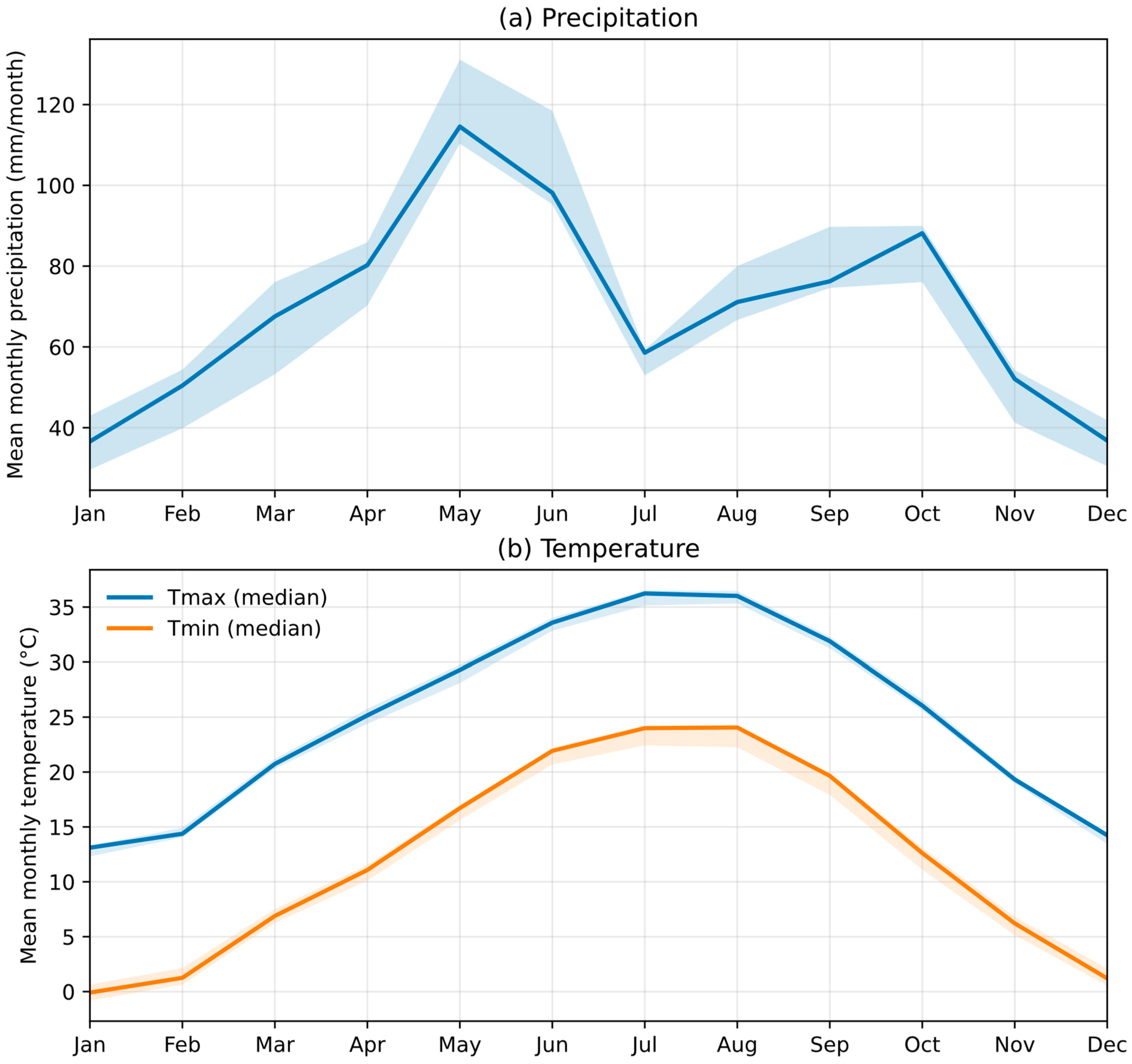
Mean annual precipitation ranged from 750 to 891 mm across stations (2.05–2.44 mm/day on average), with the wettest conditions at the Prism1 and Prism2 grid points (~886–891 mm) and the driest at Markley (~750 mm) (Figure 3a). Rainfall was seasonally concentrated, with a late-spring maximum (May median ≈ 115 mm/month across stations) and a secondary peak in early fall (October median ≈ 88 mm/month), whereas winter totals (December–January) were typically lowest (≈37 mm/month). Precipitation was event-driven and strongly right-skewed; across stations, the wettest 5% of rainy days contributed ~30–34% of total precipitation.
Analysis of historical climate data (2003–2022) across the seven stations/grid points shows a coherent seasonal temperature cycle across the Eagle Mountain Lake watershed (Figure 3b). Mean annual temperature ranges from 17.8 to 19.0 °C across stations. Monthly mean maximum temperature ranges from 12.3 to 13.3 °C in January to 35.1 to 36.5 °C in July, while monthly mean minimum temperature ranges from −0.8 to 0.6 °C in January to 22.3 to 24.2 °C in August. The PRISM grid points (Prism1 and Prism2) are slightly cooler than the station observations, consistent with their gridded spatial averaging.
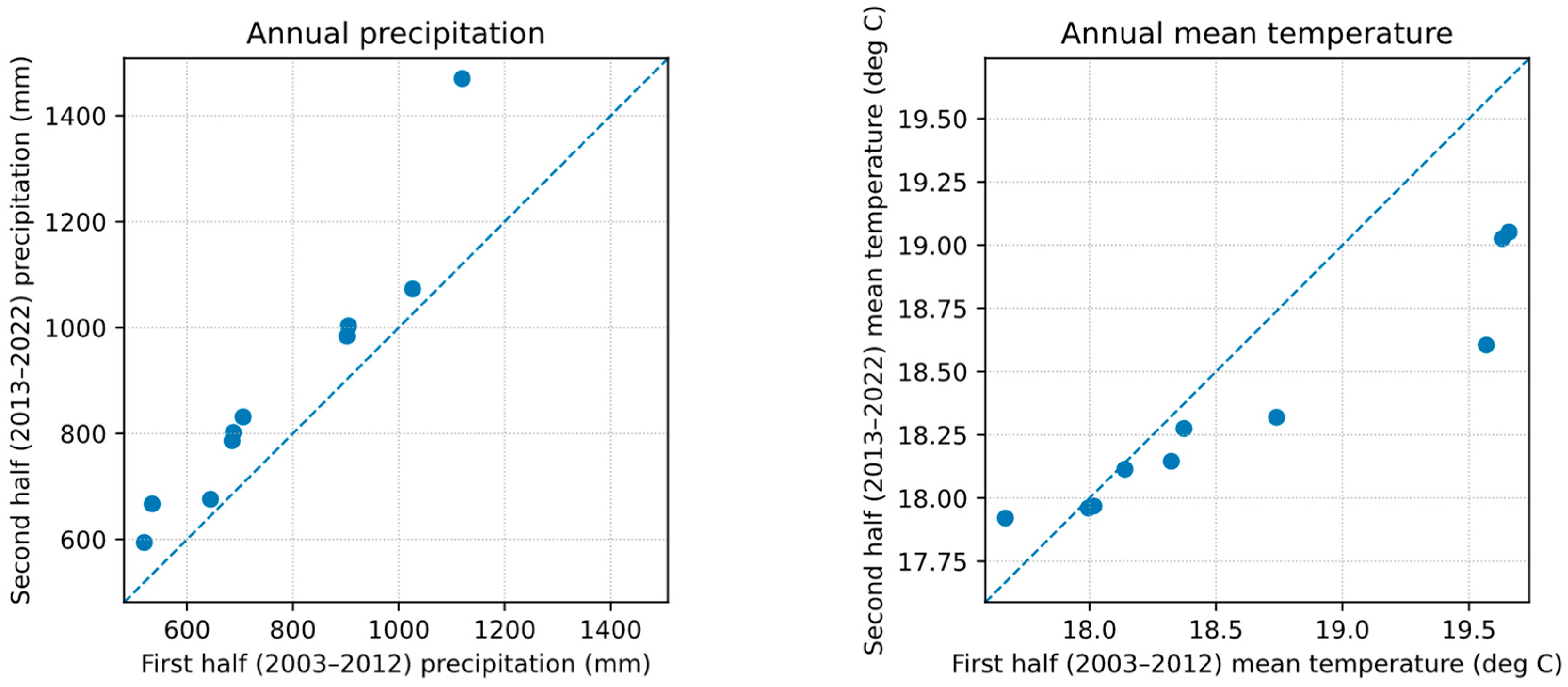
Time series diagnostics of the baseline climate inputs indicated that, over the 2003–2022 period, annual basin-average precipitation showed a modest upward shift in the latter half of the record, whereas annual mean temperature showed no strong monotonic trend. ITA plots (Appendix A, Figure A1) suggest that wetter years were somewhat more frequent in 2013–2022 than in 2003–2012, while temperature values clustered near the 1:1 line. Pettitt tests applied to annual precipitation and temperature did not identify statistically significant change points (p > 0.05), indicating that the baseline series were reasonably homogeneous for use as a reference period.
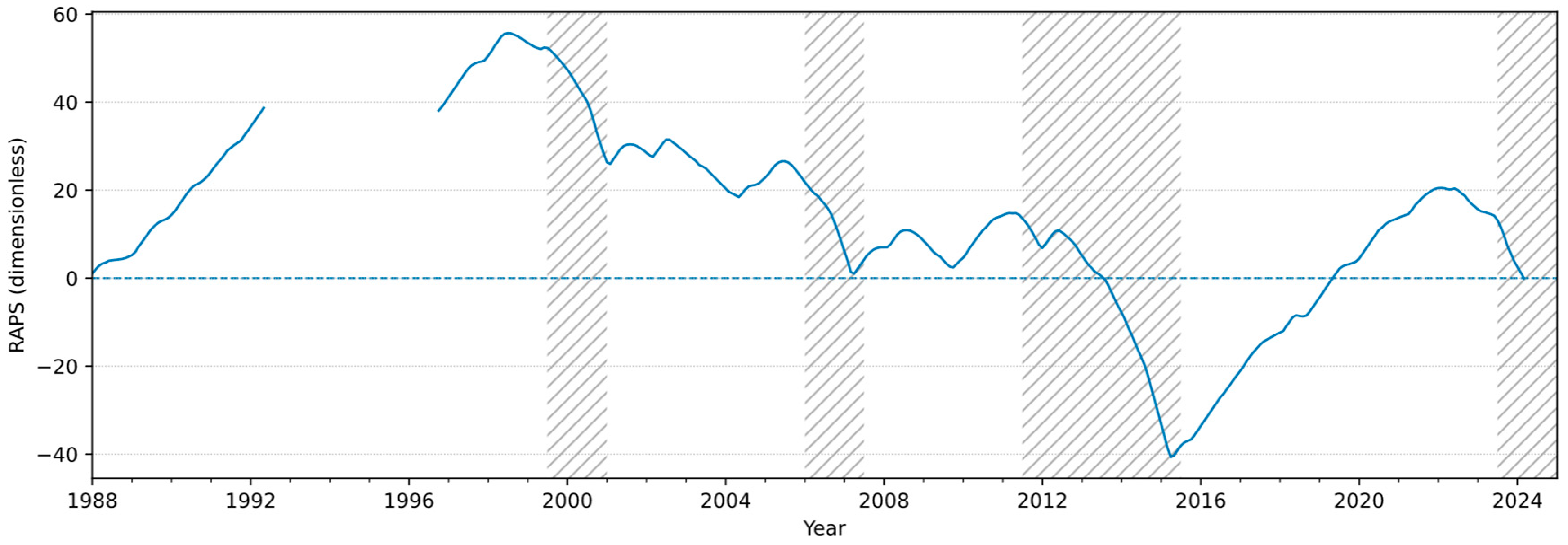
The RAPS diagnostic of monthly conservation storage (Figure A2) showed clear multi-year persistence and regime-like shifts in Eagle Mountain Lake storage rather than isolated, single-season anomalies. The RAPS trajectory increased through the early record, indicating a sustained period of above-average storage, then transitioned into pronounced downward segments that coincide with the major low-storage episodes (mid–1999 to mid–2000 and mid–2006 to mid–2007). The longest and steepest decline occurred from mid-2011 to mid-2015, culminating in the most negative RAPS values and confirming the drought of record as the dominant storage drawdown event in the series. After mid-2015, the RAPS curve shifted upward again, reflecting a multi-year recovery toward above-average storage, followed by a renewed downturn beginning in mid-2023, consistent with the recent low-storage period. Overall, the RAPS results reinforce that storage risk is governed by persistent multi-year deficits, supporting our emphasis on duration-based threshold metrics and persistence-focused indicators.

3.3. Projected Climate Changes

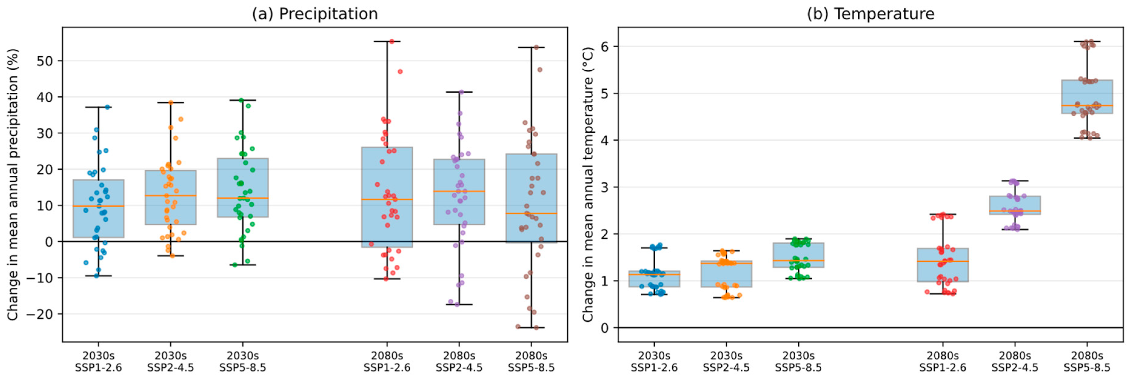
Projected precipitation changes were less consistent than temperature (Figure 4). Across stations and GCMs, median changes in mean annual precipitation were modestly positive, but the ensemble range spanned about 10–24% decreases and 37–55% increases, depending on scenario and horizon (Figure 4a; Table A6). The spread was larger in the 2080s than in the 2030s because inter-model divergence increases under stronger forcing and because precipitation responses in the south-central United States remain dominated by model-to-model differences in circulation and convective processes. Monthly and seasonal precipitation change patterns are summarized in Figure A3 and Figure A4, and station-level baseline precipitation and percent changes are provided in Table A7. All five CMIP6 GCMs projected warming across all seven stations/grid points. Relative to the 2003–2022 baseline, mean annual temperature increased by 0.7–1.9 °C in the 2030s (2031–2050) and by 0.7–6.1 °C in the 2080s (2081–2100), with larger warming under higher-emission pathways (Figure 4b; Table A8).

3.4. Projected Streamflow Changes

3.4.1. Annual Streamflow

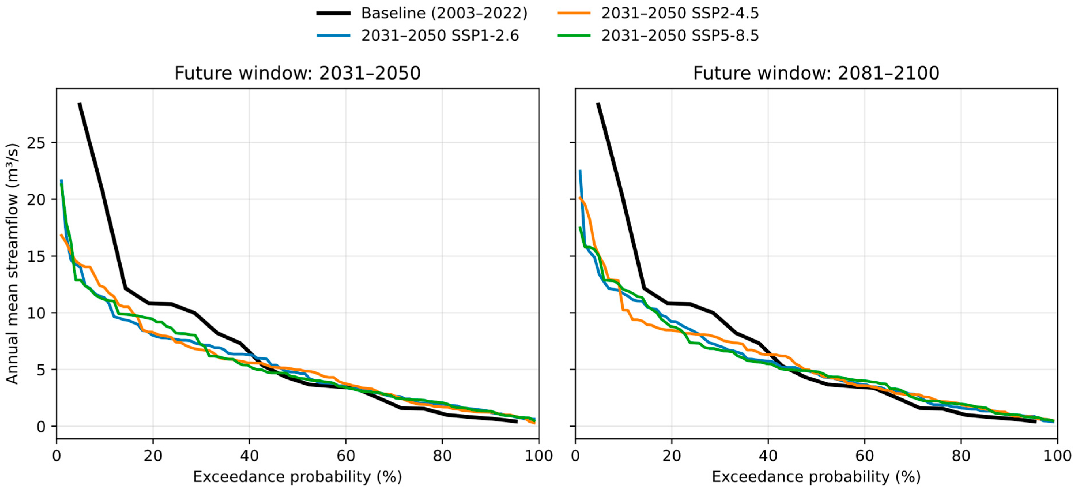
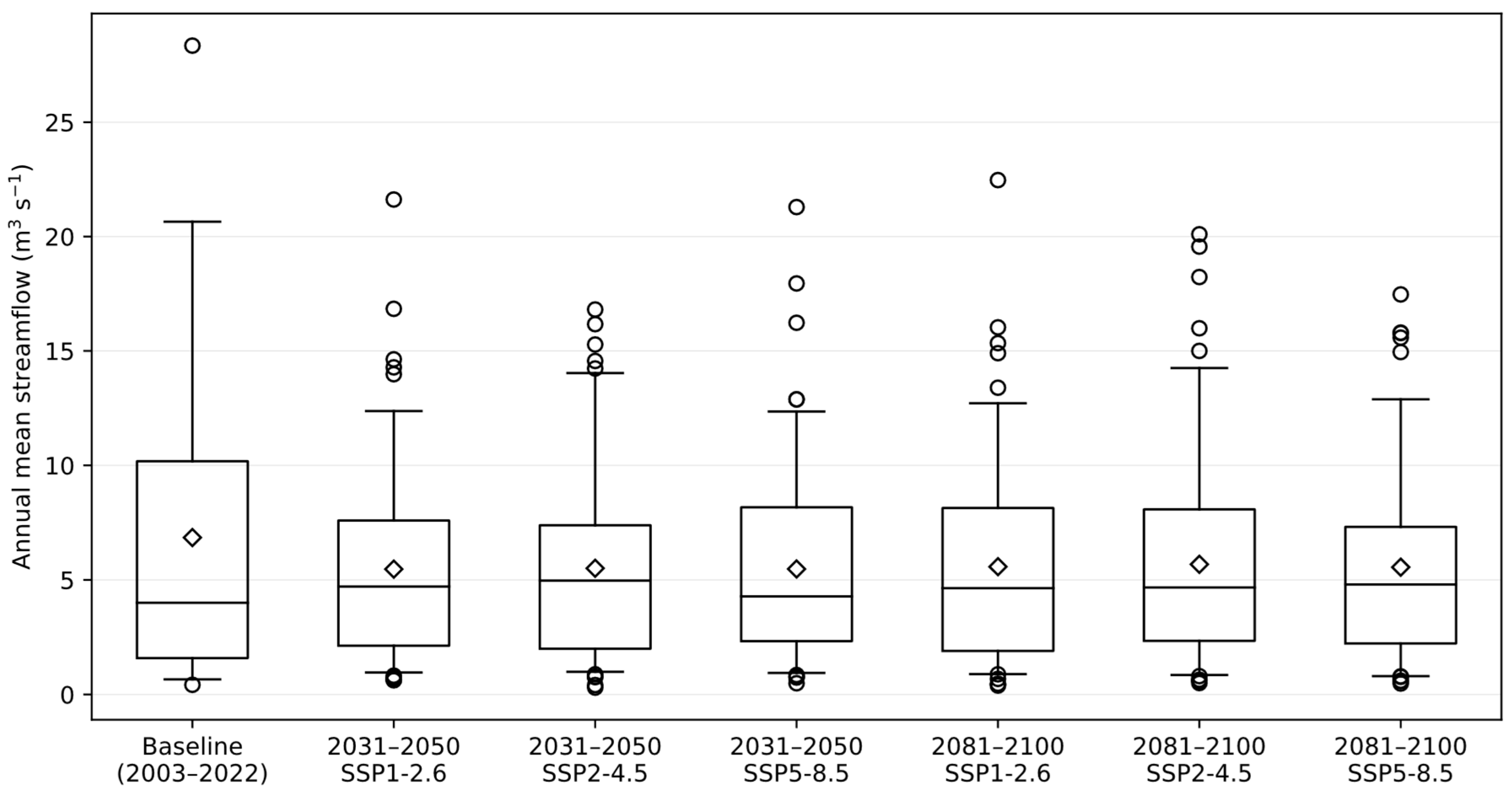
SWAT simulations indicated consistent declines in mean annual streamflow across scenarios and time horizons (Table 3; Figure 5). Although several climate projections suggested neutral-to-increasing precipitation, increased evaporative demand and altered runoff partitioning reduced net runoff generation, thereby lowering mean inflows at the Eagle Mountain Lake outlet. Flow duration curves similarly shifted downward across most exceedance probabilities, indicating broad-based reductions in low-to-median flows (Figure A5).
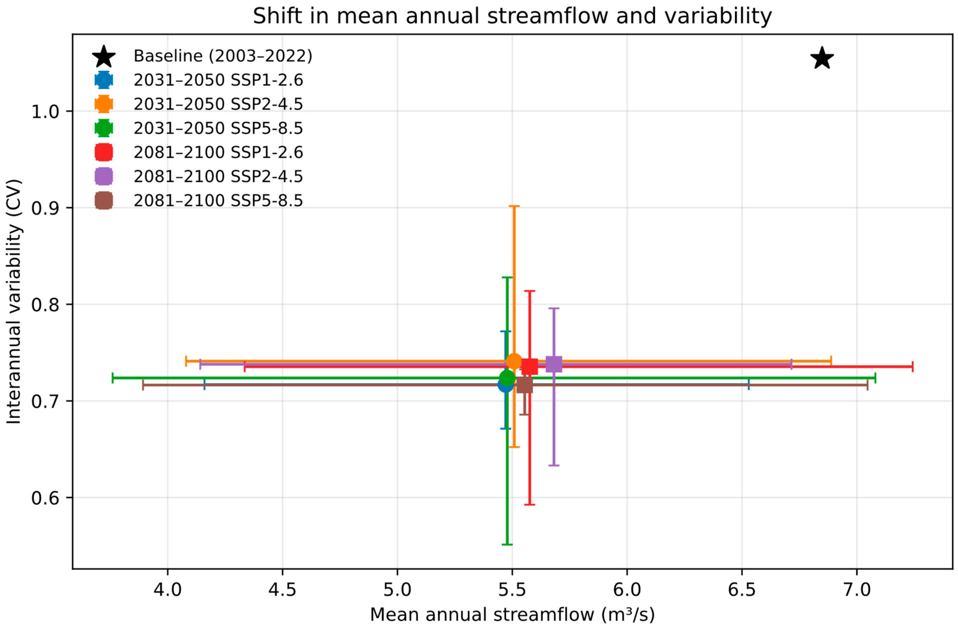
By the 2080s, average annual streamflow was projected to decline to 5.55–5.68 m3/s, representing reductions of 17.0–18.9% relative to historical conditions. Notably, SSP2-4.5 projected the smallest reduction (−17.0%), while SSP5-8.5 projected the largest (−18.9%). This counterintuitive pattern, in which the moderate-emission scenario yielded smaller streamflow reductions than the low-emission scenario, reflects the complex interplay between increased precipitation and enhanced evapotranspiration at varying levels of warming.

3.4.2. Seasonal and Monthly Streamflow

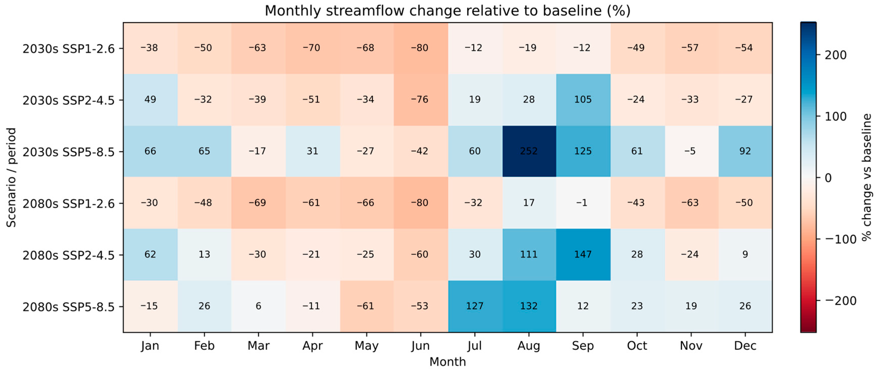
Monthly streamflow projections revealed pronounced seasonal redistribution of inflows (Figure 6). Under SSP1-2.6, reductions were concentrated in late spring and early summer, with June decreases approaching 80% in both the 2030s and 2080s ensemble means. Under SSP2-4.5, spring and early summer reductions persisted but were partially offset by increases in early fall in the 2080s (e.g., September). SSP5-8.5 exhibited the most heterogeneous monthly response, including substantial late-summer increases in some months and time horizons. Uncertainty bounds across GCMs for monthly and seasonal percent changes are provided in Table A9 and Table A10, and additional seasonal and variability diagnostics are shown in Figure A6 and Figure A7.
Higher-emission scenarios showed mixed monthly responses. For example, the 2030s SSP5-8.5 ensemble mean indicated increases in several months, including August (+252%) and December (+92%) relative to baseline, while other months declined (Figure 6). In the 2080s, SSP5-8.5 produced very large late-summer increases (July–August > +100% ensemble mean) but continued reductions in spring and early summer (e.g., May–June). Operationally, this seasonal shift suggests greater late-summer inflow volumes and a higher likelihood of storm-driven inflow pulses during the peak demand season. These patterns imply greater intra-annual variability and heightened operational complexity for reservoir management under high emissions.
Aggregated by season, March–May (spring) streamflow was projected to decline strongly (about 39% on average across scenarios), and June–August (summer) streamflow showed the widest relative spread because baseline flows were low. These shifts have direct operational relevance: the largest reductions occurred during the typical refill season (spring through early summer), which reduced the probability of recovering storage before peak summer demand. Conversely, projected relative increases in July–September under some scenarios reflected occasional convective storm clusters rather than sustained baseflow, which can complicate operations by increasing short-duration flood risk without reliably improving seasonal water supply reliability.

3.5. Observed Reservoir Storage Dynamics and Threshold-Based Performance

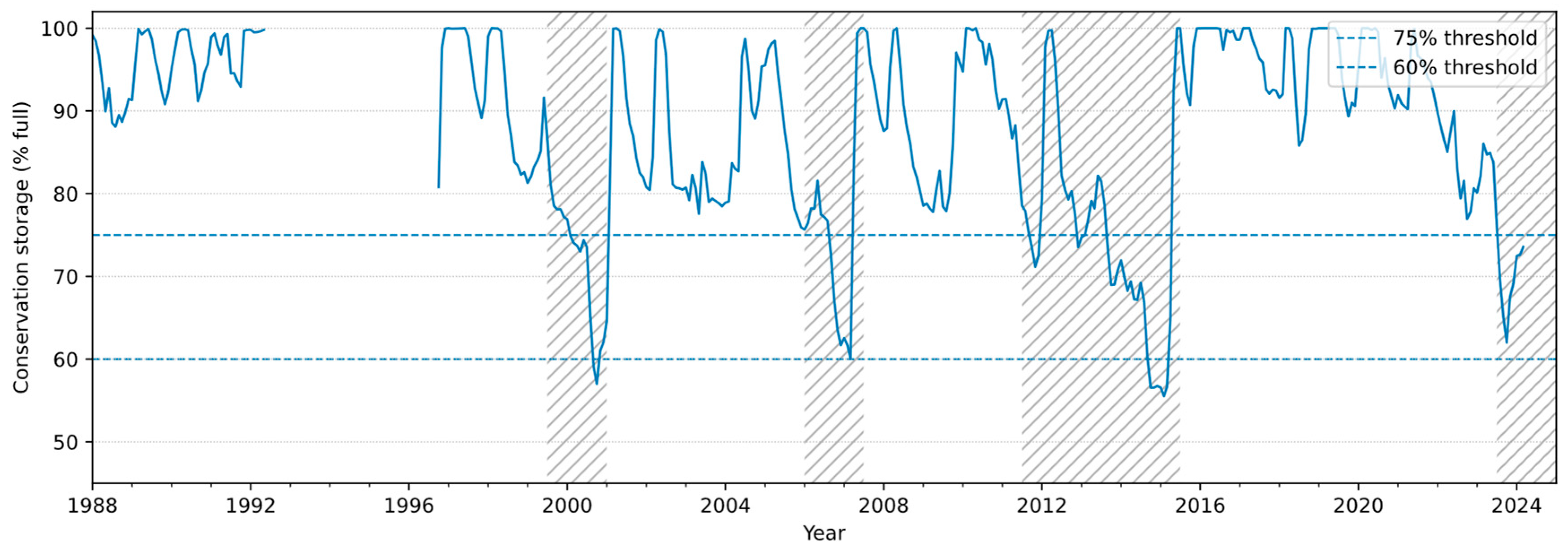
Historical observations provide an operational benchmark for interpreting projected changes in inflow. Across 1988–2024, monthly conservation storage was typically near full pool but exhibited episodic multi-month to multi-year drawdowns (Figure 7). Hatched bands highlight four sustained low-storage episodes in the available record: mid-1999 to 2000, 2006 to mid-2007, mid-2011 to mid-2015 (during the 2010–2015 Texas drought), and mid-2023 through 2024. These clusters support the use of multi-year persistence metrics (e.g., rolling multi-year inflow anomalies) rather than single-year totals alone. The lowest monthly mean storage occurred in January 2015 (55.5% full), and the lowest daily storage reached 53.7% full on 27 January 2015 during the drought of record [21,26].
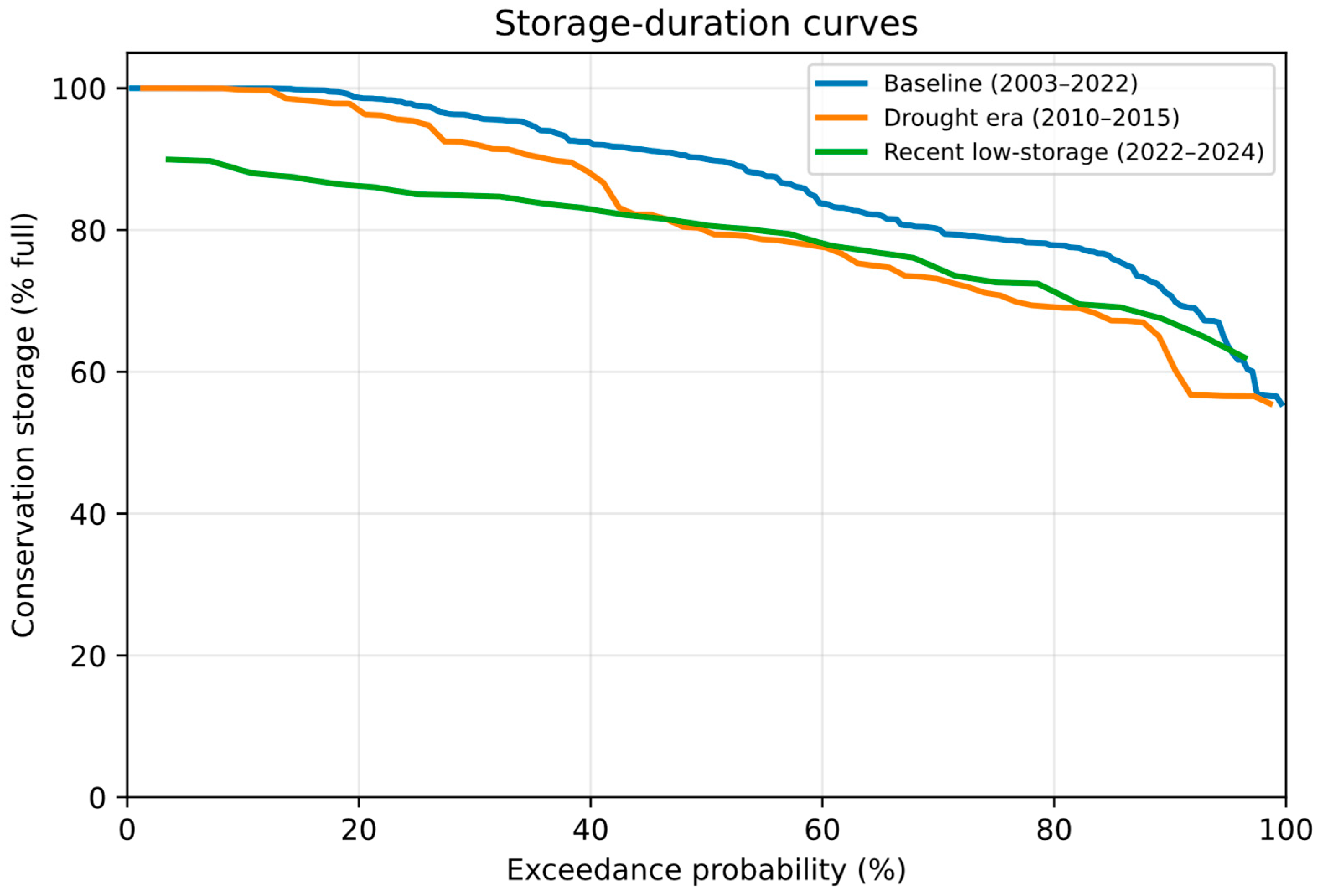
Threshold-based performance metrics showed that low-storage conditions could persist for multiple seasons once drawdown began (Table 4). During the 2003–2022 baseline period, storage remained at or above 75% in 86% of months, but the longest consecutive period below 75% lasted 20 months (September 2013–April 2015). During the 2010–2015 drought, reliability at the 75% threshold declined to 64% of months (26 of 72 below 75%). Storage fell below 60% for six consecutive months (October 2014–March 2015). When storage was below 75%, the average shortfall relative to the 75% threshold was about 8–9 percentage points, corresponding to roughly 18–20 × 106 m3 of conserved storage depending on the conservation capacity reference.
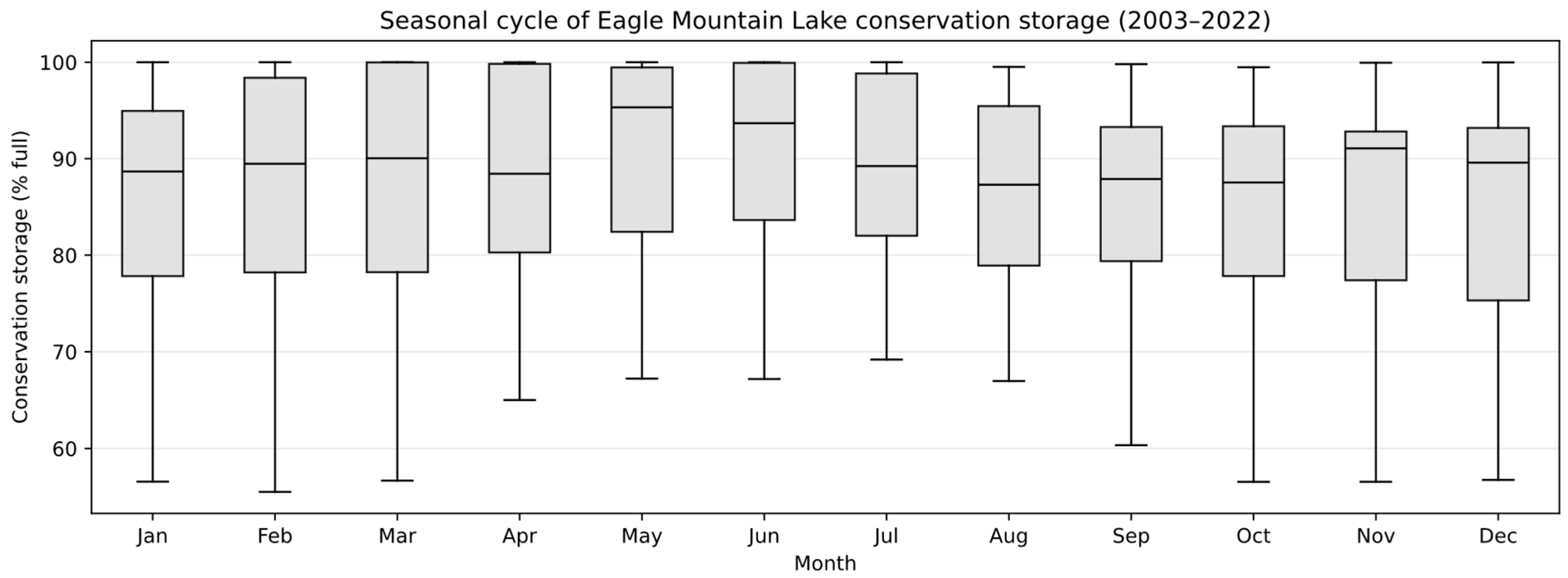
Storage duration curves illustrated changes in the full distribution of conditions, not only the minimum (Figure 8). Compared with the baseline distribution, drought-era storage exhibited a substantially higher probability of being below 75% full, consistent with extended periods of reduced inflow and/or higher losses. Seasonally, the reservoir tended to reach its annual maximum in winter to early summer (January–June in 29 of 34 years) and its annual minimum in late summer to early winter (October–December in 20 of 34 years), consistent with a spring refill followed by summer drawdown (Figure A8).

3.6. Translating Projected Inflows into Reservoir Operations Risk

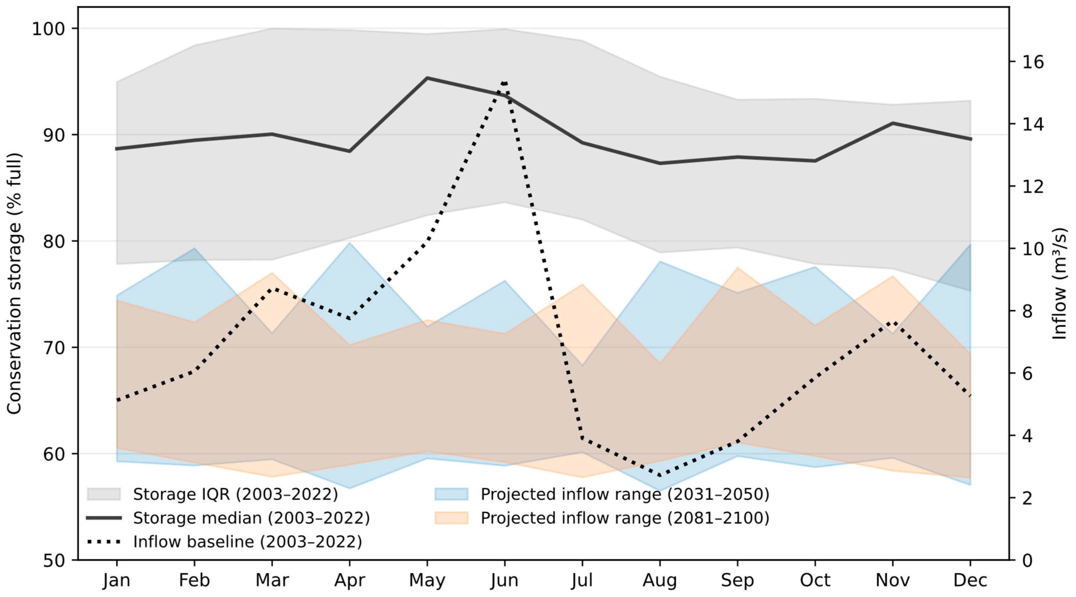
Projected inflow changes are most actionable when expressed as storage-based indicators that align with reservoir management practices. Two features of the historical record guide interpretation: (i) Eagle Mountain Lake typically refilled in late winter through early summer, and (ii) the most severe drawdowns occurred when inflow deficits persisted across multiple years.
Figure 9 overlays the observed seasonal storage cycle (2003–2022) with projected monthly inflow shifts. Storage was typically highest in May–June, consistent with the historical refill season, and declined through late summer and early fall. SWAT projections indicated that the largest inflow reductions occurred in March–June across scenarios, weakening the refill signal that builds storage heading into the warm season.
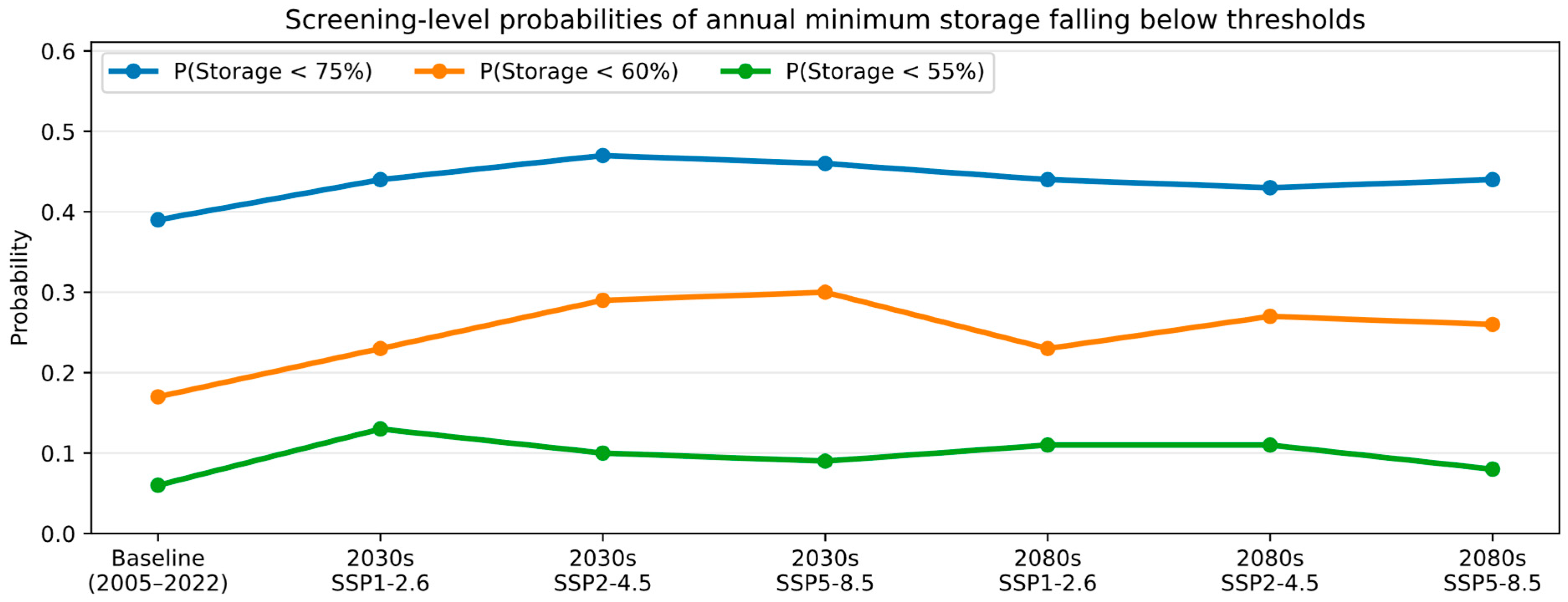
Using the historical relationship between multi-year inflow deficits and annual minimum storage, the screening results (Table 5) indicated a higher likelihood of severe low-storage years in the future.
Relative to the baseline (2003–2022), the inferred probability of annual minimum storage dropping below 60% increased from 0.17 to approximately 0.23–0.30 across scenarios, and the probability of dropping below 55% increased from 0.06 to approximately 0.08–0.13 (Figure 10). These changes reflect storage’s sensitivity to sustained inflow deficits rather than to single-year anomalies.
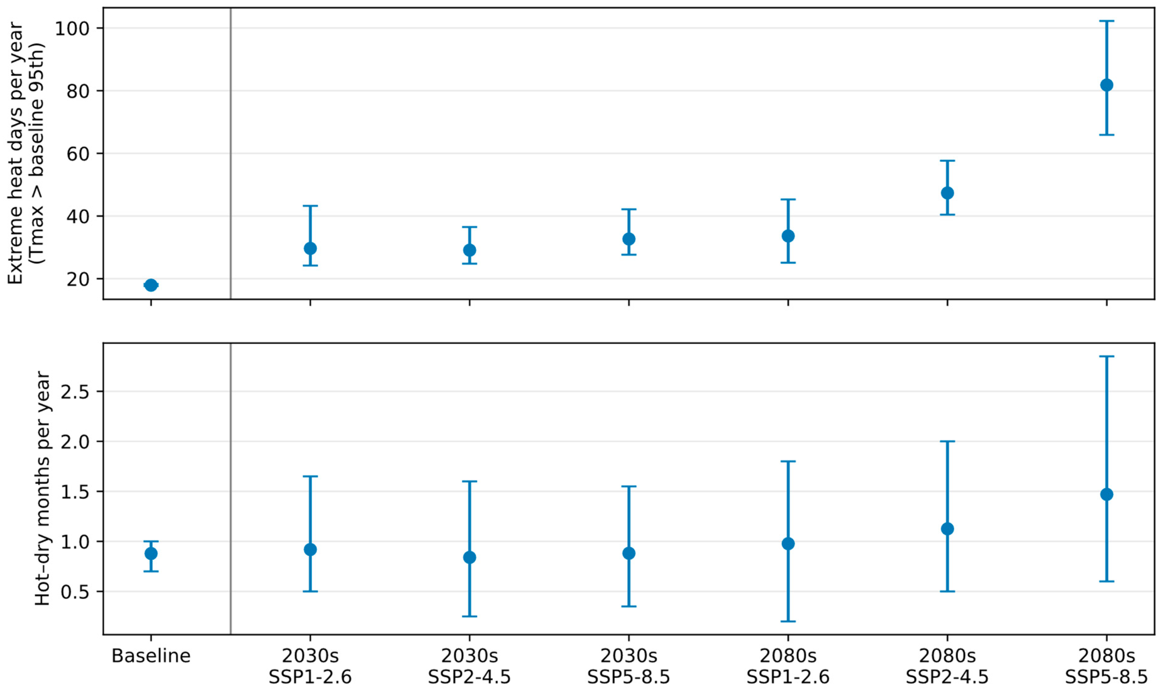
To align with management practice, climate stress was framed as the frequency of “hot–dry months”, months with unusually high temperatures (monthly mean Tmax above the 2003–2022 90th percentile) and below-normal rainfall (monthly precipitation below the baseline median). Across stations, the historical baseline averages ~0.9 hot–dry months yr−1. Ensemble projections indicated little change by the 2030s (0.84–0.92 hot–dry months yr−1 across SSPs) but an apparent increase by the 2080s, especially under SSP5-8.5 (~1.47 hot–dry months yr−1; range across station-GCM combinations 0.60–2.85). In parallel, extreme heat days (Tmax above the baseline 95th percentile) increased from ~18 days yr−1 to ~30–33 days yr−1 in the 2030s and to ~34–82 days yr−1 in the 2080s (Figure 11). These shifts aligned with SWAT-projected March–June inflow reductions and directly map to observed operating behavior: hot–dry months coincided with higher water supply releases and lower lake levels, tightening the margin between refill, summer demand, and flood readiness (Section 3.7).

3.7. Observed Reservoir Operations Signals and Climate Triggers

The operations record provides a direct link between climate conditions and the decisions that control lake levels. During the overlap period with the daily climate record (2003–2021), water supply releases and lake levels exhibited a clear warm-season signal, while flood discharges occurred in distinct episodes associated with high lake levels and multi-day rainfall.
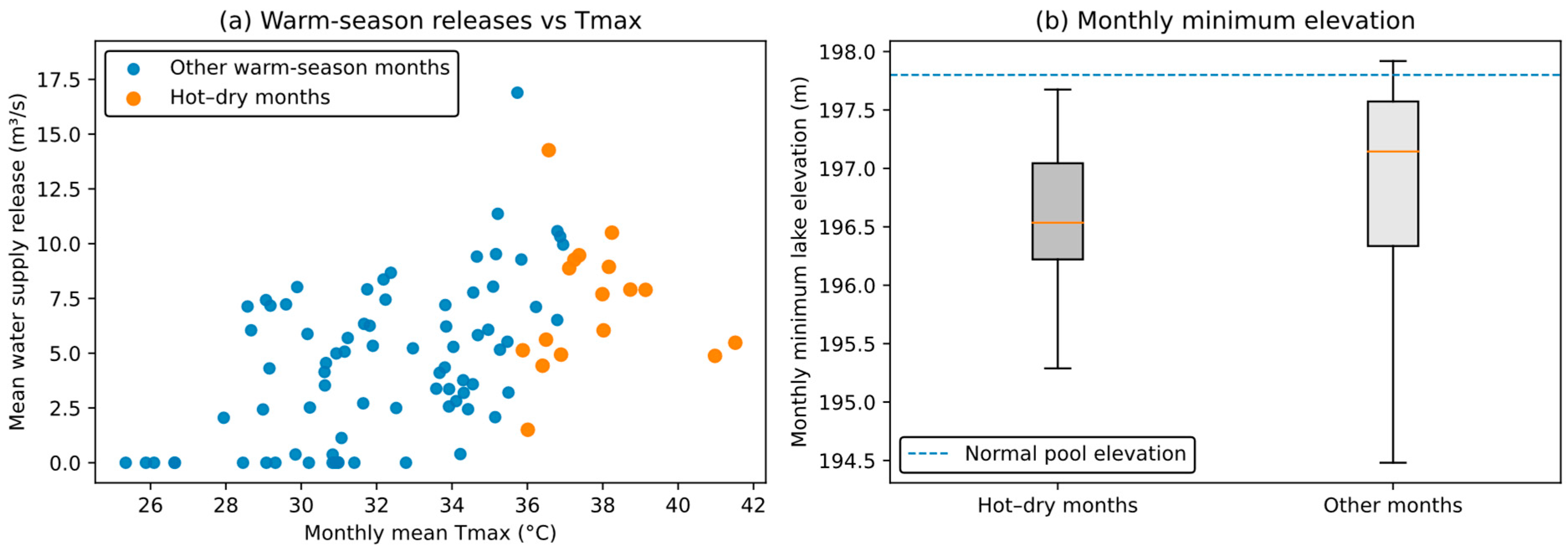
Hot–dry months are rare but operationally important: compared with all other months, hot–dry months had approximately double the mean water supply release (7.2 vs. 3.5 m3/s, equivalent to 255 vs. 122 ft3/s; Mann–Whitney p = 1.4 × 10⁻⁵) and a lower monthly minimum lake level (about 0.30 m lower on average; p = 0.041). These patterns are consistent with peak demand conditions occurring when inflows are typically low (Figure 12).
A simple warm-season regression quantifies the release sensitivity: within May–September, monthly mean water supply release increased by approximately 0.36 m3 s−1 per +1 °C increase in monthly mean Tmax (p = 0.004) and decreased by about 0.018 m3 s−1 per +1 mm increase in monthly precipitation (p = 0.010). This temperature and dryness signal provides an operational interpretation for the projected increase in extreme heat days and hot–dry months.
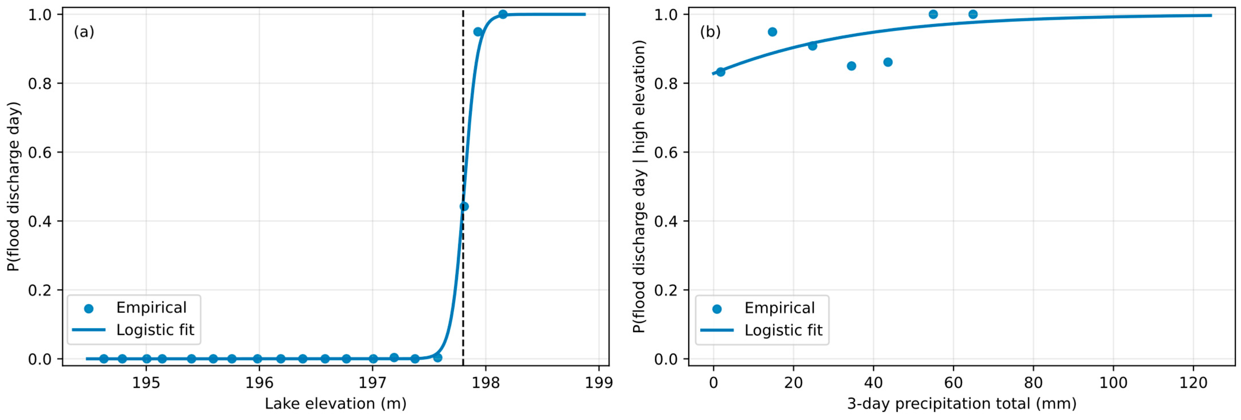
Flood discharges show a different operating mode. Flood releases occur primarily when lake levels are at or above the normal pool elevation and when multi-day rainfall totals are elevated. A logistic model using only lake level and a 3-day precipitation total reproduced daily flood release occurrence with high skill (5-fold time series cross-validation AUC = 0.99; Brier score = 0.04), indicating that flood releases were tightly controlled by hydrologic triggers that can be summarized without complex modeling (Figure 13).

4. Discussion

This section synthesizes the results in the context of the study objectives: (i) evaluating SWAT performance for the Upper West Fork Trinity watershed, (ii) characterizing downscaled CMIP6 climate drivers and their uncertainty, (iii) translating those drivers into seasonal inflow shifts, and (iv) interpreting operational implications for Eagle Mountain Lake using threshold-based storage metrics and observed release/discharge responses to climate stressors.

4.1. Model Performance in Context

The calibrated SWAT model demonstrated satisfactory to good performance in reproducing observed streamflow dynamics at multiple locations within the Upper West Fork Trinity Watershed. Validation metrics for subbasin 22 (R2 = 0.72; NSE = 0.72; KGE = 0.80) compare favorably with other SWAT applications in Texas and similar regions. Tefera and Ray [38] reported R2 = 0.65 and NSE = 0.61 for the Bosque watershed in North-Central Texas, while Chen et al. [39] achieved R2 = 0.70 and NSE = 0.79 in the Upper Mississippi River basin. The robust validation performance provides confidence in the model’s ability to analyze climate change scenarios.
The most sensitive parameters (CN2, ESCO, GW_REVAP, GW_DELAY, and related groundwater recession terms) are consistent with many SWAT applications in Texas and other semi-humid, mixed land use basins. Runoff sensitivity to CN2 and soil/evaporation parameters reflects the importance of infiltration-excess runoff and evapotranspiration partitioning, while sensitivity to groundwater parameters reflects the role of shallow aquifer storage in sustaining baseflow during dry periods. Similar sensitivity patterns have been reported for SWAT-based climate impact studies in Texas, including the Bosque watershed and other regional basins [38,40]. These consistencies provide confidence that the calibrated parameter set reflects plausible process controls rather than compensating errors.

4.2. Climate Projections and Uncertainty

The downscaled daily series showed a robust warming signal across all stations and GCMs. Relative to 2003–2022, mean annual temperature increased by 0.7–1.9 °C by the 2030s and by 0.7–6.1 °C by the 2080s, depending on SSP (Table A6). Importantly for operations, warming is not only reflected in a higher mean but also in many more very hot days: days above the historical 95th percentile increased from ~18 yr−1 to ~30–33 yr−1 in the 2030s and to ~34–82 yr−1 in the 2080s (Figure 11).
Precipitation projections remained more uncertain than temperature. The ensemble median indicated modest increases in mean annual precipitation (~10–14%), but the full range spans decreases of ~10–24% and increases up to ~55% (Figure 4; Table A7). This uncertainty matters because relatively small changes in rainfall timing and intensity can translate into larger changes in runoff generation and seasonal refill, particularly when paired with higher evaporative demand in a warmer atmosphere.

4.3. Streamflow Response Mechanisms

The projected decline in annual streamflow despite modest increases in mean annual precipitation in some scenarios indicates that warming-driven increases in evaporative demand can dominate the water balance. The temperature signal was robust across stations and GCMs (Figure 4b), and higher temperatures increase potential evapotranspiration and reduce effective precipitation available for runoff generation, particularly during the warm season. Accordingly, precipitation variability alone is insufficient to explain simulated flow reductions; the combined influence of warming, longer growing seasons, and higher atmospheric demand provides a physically consistent explanation for reduced runoff efficiency.
The seasonal redistribution of streamflow, with enhanced reductions in spring–summer and potential increases in late summer–fall, reflects the projected changes in precipitation seasonality combined with temperature-driven evapotranspiration dynamics. Spring streamflow reductions of up to 80% (June under SSP1-2.6) would substantially impact the primary reservoir recharge period, potentially leading to critically low water levels during subsequent summer demand peaks. Conversely, projected late-summer and fall increases (>250% in August under some scenarios) could increase flood risk while providing limited water supply benefit if reservoir storage is already depleted.

4.4. Comparison with Regional Studies

The projected streamflow reductions in the Upper West Fork Trinity watershed are broadly consistent with recent Texas-focused and southern Great Plains studies that emphasize increasing evaporative demand and more persistent drought risk under warming. For example, drought risk assessments for multiple Texas reservoirs have shown that storage outcomes can diverge across climate models and that explicitly tracking critical storage thresholds improves interpretability for planning [41]. At the basin scale, SWAT-based work in the Trinity River basin has similarly highlighted the value of process-based simulations for interpreting future streamflow drought behavior under changing climate forcing [42].
Nationally, the magnitude and direction of projected inflow changes align with broader evidence that many U.S. reservoirs will experience reduced inflows and increased hydroclimatic stress as temperatures rise [43]. The seasonality signal identified here, with larger reductions during the spring refill period and higher relative variability in late summer, is also consistent with studies across the Southwest and southern Great Plains that project earlier and less reliable runoff generation under warming, even when precipitation changes are uncertain [17,44].

4.5. Implications for Water Resource Management

The projected 17–20% reduction in average annual streamflow, combined with a marked increase in extreme heat days and more frequent hot–dry months, has direct implications for future reservoir operations at Eagle Mountain Lake. SWAT results indicated reduced spring refill (March–June), whereas daily climate projections indicated that hot conditions would intensify during the warm season. Because observed operations indicated that hot–dry months coincided with roughly twice the mean water supply release and lower minimum lake levels (Section 3.7), these climate shifts would increase the likelihood of warm-season drawdown and tighter operating margins even if operating rules remain unchanged.
Firstly, enhanced storage and capture infrastructure could maximize the retention of projected increases in late-summer and fall streamflow. Upgrades to intake structures, spillway capacity, and pumping systems could enable rapid response to episodic high-flow events that may occur more frequently under climate change scenarios. From a flood operations perspective, the projected late-summer inflow increases imply that the period requiring available flood storage and rapid release capacity may extend into July–September. Under the scenario with the largest late-summer increases (2030s SSP5-8.5), the ensemble mean July–September inflow volume would be approximately 3.7 × 10⁷ m3 higher than baseline, about 15% of the reservoir’s conservation storage. Although these estimates are based on mean monthly inflows and do not represent peak event flows, they indicate a higher likelihood that a small number of intense storms could rapidly raise the pool elevation and trigger flood releases if the reservoir is near normal pool elevation. Practically, this supports (i) maintaining seasonal flood buffer space later into summer, (ii) prioritizing forecast-informed pre-releases when heavy rainfall is expected and the pool is elevated, and (iii) revisiting downstream release constraints and spillway/outlet capacities to ensure safe routing of late-summer storm clusters.
Secondly, demand management and conservation programs will become increasingly critical as supply margins narrow. The DFW region has already achieved per-capita water use reductions (541 L/day vs. the state average of 587 L/day), and further conservation, particularly in outdoor irrigation, which accounts for 27% of urban use, could substantially buffer against projected supply reductions. Thirdly, diversification of water supply sources through enhanced conjunctive use of surface and groundwater, water reuse and recycling, and interbasin transfer agreements could reduce vulnerability to disruptions in single-source supply. The Texas 2022 State Water Plan identifies multiple regional water supply strategies that could complement the supply of Eagle Mountain Lake under future climate conditions. Fourthly, updated reservoir operating rules that account for changes in seasonal streamflow patterns could improve water supply reliability. Current operations, developed under historical climate conditions, may require revision to optimize storage and releases in response to projected seasonal shifts in inflow timing and magnitude.
Finally, communicating risk in operational terms is as important as the hydrologic signal itself. The “hot–dry month” framing translates climate projections into the months that matter most for managers, periods with peak demand and typically low inflows, and the operations record confirms that these months are associated with higher releases and lower lake levels. In parallel, flood discharges occur primarily when lake levels are near or above normal pool and after multi-day rainfall clusters (AUC = 0.99), underscoring that future operations will need to balance refill and drought protection against maintaining flood buffer. Together, these results support drought triggers and rule curve reviews that account for both seasonal timing shifts and persistence of hot, dry conditions.

4.6. Storage Reliability Implications from Reservoir Observations

Reservoir observations provide a practical lens for interpreting the projected inflow changes. The 2010–2015 Texas drought produced the longest and deepest drawdown in the 1988–2024 record, including 20 months below 75% storage and a minimum of about 54% full. These durations are operationally critical because they span multiple high-demand seasons and reduce flexibility for meeting competing water supply and recreational objectives.
Projected inflow reductions would be largest in March–June, which coincides with the period when the reservoir most often reaches its annual maximum and refills from watershed inflows (Figure A8). This seasonal alignment suggests that changes in inflow timing can increase the persistence of late-summer low-storage levels unless offset by operational adjustments (e.g., revised release rules, drought-stage demand reductions, increased reuse, or additional interconnections). Although this study does not simulate reservoir operations, the threshold metrics reported here provide transparent benchmarks (75% and 60% storage) that can be used to evaluate future reservoir performance once SWAT inflow projections are coupled to an operations model.
The screening-level storage risk emulator developed here provides a transparent method for translating inflow projections into storage outcomes, using observed behavior as a benchmark. Although it does not replace an explicit reservoir operations model, it captures a key operational reality: minimum storage is strongly associated with sustained inflow deficits over multiple years. Under both mid-century and late-century horizons, the projected inflow distributions imply higher probabilities of severe low-storage years (Smin < 60%) than the historical baseline (Table 5), even when mean annual precipitation does not decline consistently across models.
This approach also supports “stress testing” that is directly actionable. For example, utilities can interpret the probabilities in Figure 10 as the likelihood of entering restriction-relevant storage zones under unchanged operations and demand. When combined with the compound hot–dry month lens (hot conditions plus below-normal rainfall), the results indicated a higher risk of demand–supply mismatch in the warm season: storage refilled less during spring and then faced higher evaporative and demand pressures during summer. These dynamics motivate adaptive rule curves, enhanced conservation, and diversified supply portfolios designed for persistence-driven drought rather than isolated low-flow years.

4.7. Study Limitations and Future Research

Some limitations should be considered when interpreting these results. Firstly, potential evapotranspiration was estimated using the Hargreaves method because humidity, wind speed, and solar radiation data were not consistently available across stations. Although a sensitivity check indicated modest effects on simulated streamflow, using the Penman–Monteith method where feasible would reduce uncertainty in warm-season water balance estimates. Secondly, land cover was held constant and therefore does not represent projected land use change in the rapidly urbanizing Dallas–Fort Worth region, which could alter runoff generation, infiltration, and baseflow. Thirdly, the analysis emphasized annual and monthly statistics to support long-term planning, which may not fully capture short-duration extremes and persistence (e.g., multi-day flood-producing storms or multi-week hot–dry spells) that drive operational stress. Fourthly, future reservoir storage and releases were not simulated using an explicit reservoir mass balance model and operating policy, and potential changes in human water use (demand growth, irrigation practices, groundwater pumping) were not explicitly represented. A mid-century 2051–2080 window was not analyzed because the downscaled daily forcing series generated for this study covered 2031–2050 and 2081–2100; adding 2051–2080 would require regenerating the downscaled series and rerunning the SWAT ensemble, which is identified as a priority extension.
Future research should: (i) quantify daily extremes and compound event metrics directly from the downscaled daily station series, including frequency and persistence of “hot–dry” months (e.g., Tmax above the baseline 90th percentile and precipitation below the baseline median) and related run-length/clustering metrics; (ii) couple climate-conditioned SWAT inflows to a reservoir operations model (rule curve simulation and/or optimization) to evaluate storage reliability, drought trigger performance, and tradeoffs among water supply, flood risk reduction, recreation, and environmental objectives; (iii) incorporate demand growth, improved lake surface evaporation estimates under warming, and land use change scenarios; and (iv) broaden the uncertainty envelope using additional GCMs and alternative downscaling methods. Operations-focused extensions would benefit from additional data, such as daily releases (separating flood discharge and water supply releases), withdrawals, interconnection, diversion flows, and lake surface precipitation and evaporation.

5. Conclusions

By integrating a calibrated SWAT watershed model, station-scale downscaled CMIP6 daily climate projections, and a multi-decadal record of Eagle Mountain Lake storage and operations, this study translated climate-driven hydrologic change into indicators that are directly interpretable in reservoir management terms. The analytical framework emphasized three critical dimensions of climate–reservoir interactions: (i) seasonality, particularly the contrast between spring refill dynamics and warm-season drawdown patterns; (ii) persistence, focusing on multi-year inflow deficit sequences rather than isolated annual anomalies; and (iii) operational triggers, including hot–dry month conditions associated with elevated demand and rainfall clustering events linked to flood discharge protocols. Key takeaways are summarized as follows:
(1)
Projected hydroclimatic signal: Downscaled CMIP6 projections indicated robust warming across the watershed (about +0.7 to +1.9 °C in 2031–2050 and about +0.7 to +6.1 °C in 2081–2100 across scenarios), while mean annual precipitation changes remained uncertain and model-dependent.
(2)
Projected inflow change: SWAT simulations forced by the downscaled series indicated a consistent decline in mean annual inflow (about 17–20%), with the largest reductions concentrated in the spring refill season (March–June).
(3)
Storage risk implication: When inflow deficits persisted for multiple years, the historical record showed that the reservoir is more likely to enter extended low-storage episodes; screening results based on multi-year inflow anomalies indicated a higher future likelihood of crossing 75%, 60%, and 55% storage thresholds under unchanged demand and operating conditions.
(4)
Operational relevance of hot–dry months and rainfall clusters: Hot–dry months coincided with higher water supply releases and lower minimum lake levels, whereas flood discharges occurred primarily near or above normal pool and after multi-day rainfall clusters. Increasing extreme heat days and more frequent hot–dry months, therefore, tightened the operational margin between refill, summer demand, and flood readiness.
Collectively, these results indicate that the most consequential climate signal for Eagle Mountain Lake is not only “how much” inflow changes, but “when” inflow arrives and “how persistent” deficits become, because these factors govern refill reliability and the likelihood of entering storage zones associated with multi-month drawdowns. The management-oriented indicators used here (seasonal refill sensitivity, persistence-based storage risk screening, and hot–dry/rainfall cluster operational triggers) are intended as transparent, decision-relevant diagnostics; a logical next step is coupling the climate-conditioned inflow ensembles to an explicit reservoir mass balance/operations model (including demand growth and improved evaporation representation) to evaluate alternative drought triggers, rule curves, and integrated drought–flood operating strategies.
Author Contributions

Conceptualization, G.K.; methodology, G.K., D.A.A., B.L.L. and M.B.; software, G.K. and D.A.A.; validation, G.K., D.A.A., B.L.L. and M.B.; formal analysis, D.A.A. and G.K.; investigation, G.K., D.A.A., B.L.L. and M.B.; resources, G.K., B.L.L. and M.B.; data curation, G.K. and D.A.A.; writing, original draft preparation, G.K. and D.A.A.; writing, review and editing, G.K., B.L.L., T.K.C., M.B., M.S.N. and P.A.; visualization, G.K., D.A.A., M.S.N. and P.A.; supervision, G.K., B.L.L. and M.B.; project administration, G.K.; funding acquisition, G.K. All authors have read and agreed to the published version of the manuscript.

Funding

This research received no external funding.

Data Availability Statement

All data used in this study, including daily historical climate (precipitation, maximum and minimum temperature), daily future climate projections for seven stations (Alvord, Boyd, Bridgeport, Markley, Newport, PRISM1, PRISM2), the historical reservoir operations record (elevation, water supply release, flood discharge), and processed summary statistics and figure-ready datasets generated for this manuscript, will be made available upon reasonable request.

Acknowledgments

The authors thank Vinicius de Oliveira of the Tarrant Regional Water District (TRWD) for providing regional context and prior reservoir data that informed model configuration. Any remaining errors or interpretations are the responsibility of the authors. During the preparation of this manuscript, the author(s) used Grammarly (1.2.210) for the purposes of English editing, organization, and formatting. The authors have reviewed and edited the output and take full responsibility for the content of this publication.

Conflicts of Interest

The authors declare no conflicts of interest.

Abbreviations

The following abbreviations are used in this manuscript:
TRWDTarrant Regional Water District
USDAUnited States Department of Agriculture
USGSUnited States Geological Survey
US EPAUnited States Environmental Protection Agency
IPCCInternational Panel on Climate Change
CMIP6Coupled Model Intercomparison Project Phase 6
GCMGlobal Climate Model
SSPShared Socioeconomic Pathway
LARS-WGLong Ashton Research Station Weather Generator
NOAANational Oceanic and Atmospheric Administration
SWATSoil and Water Assessment Tool
SWAT-CUPSWAT Calibration and Uncertainty Programs
DEMDigital Elevation Model
HRUHydrologic Response Unit
NSENash–Sutcliffe Efficiency
KGEKling–Gupta Efficiency
RMSERoot Mean Square Error
RSRRMSE observations standard deviation ratio
CN2Curve Number for Moisture Condition II
SSURGOSoil Survey Geographic Database
PRISMParameter-elevation Regressions on Independent Slopes Model
DFWDallas–Fort Worth

Appendix A

Figure A1. Innovative trend analysis (ITA) diagnostics for baseline climate inputs (2003–2022). (left) ITA scatter plot for annual basin-average precipitation (2003–2012 vs. 2013–2022). (right) ITA scatter plot for annual basin-average mean temperature. The 1:1 line indicates no change between sub-periods; deviations indicate distributional shifts [35,37].
Hydrology 13 00063 g0a1
Figure A2. Rescaled adjusted partial sums (RAPS) of monthly Eagle Mountain Lake conservation storage (% full) for 1988–2024. Hatched shaded bands highlight sustained low-storage episodes (mid-1999 to 2000, 2006 to mid-2007, mid-2011 to mid-2015, and mid-2023 to 2024. Downward segments indicate persistent below-average storage and highlight multi-year low-storage episodes [36].
Hydrology 13 00063 g0a2
Figure A3. Median monthly precipitation change across stations (%) for each emissions pathway and time window. Values represent the median percent change across the seven stations/grid points relative to the 2003–2022 baseline. Blue indicates increases and red indicates decreases.
Hydrology 13 00063 g0a3
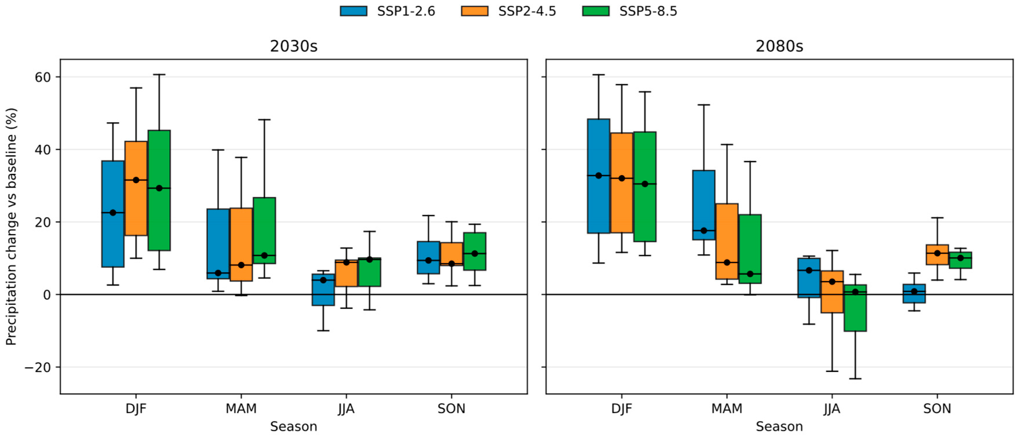
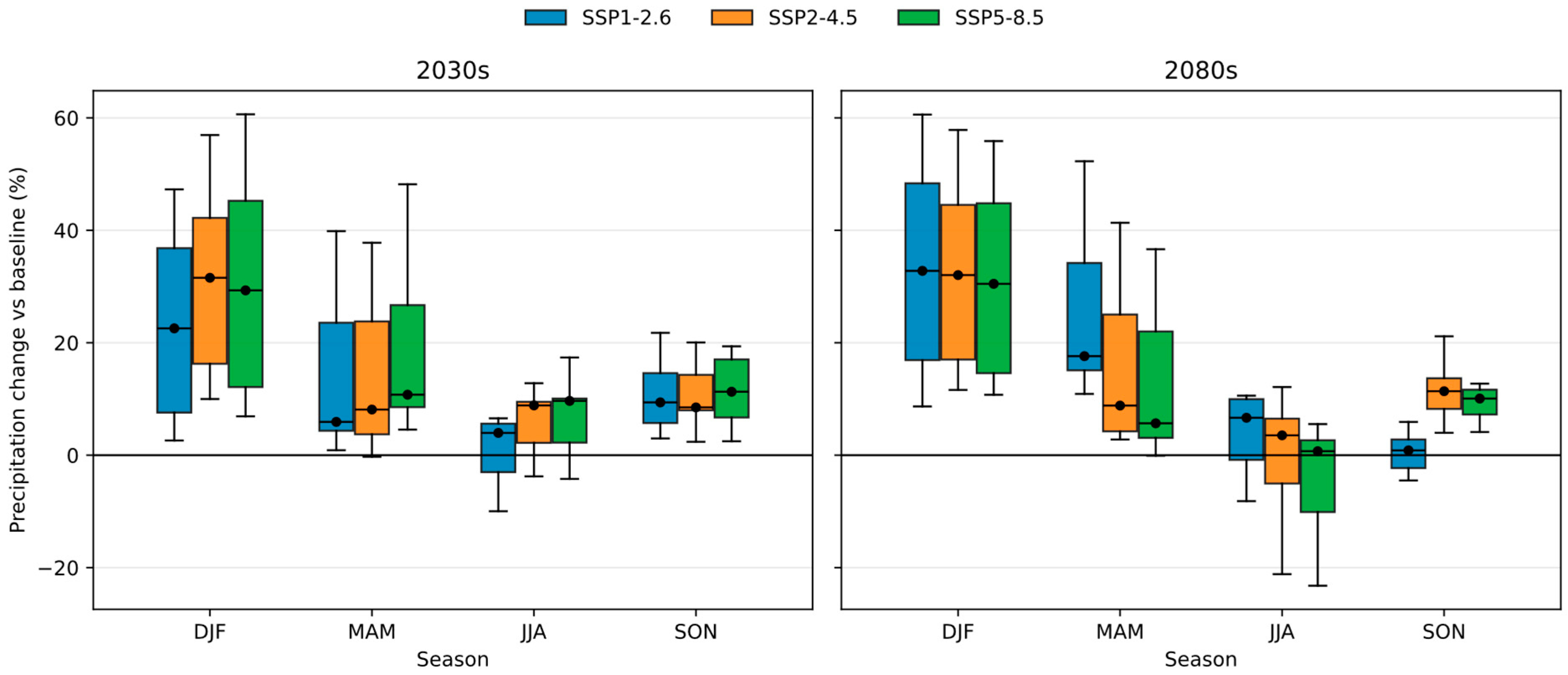
Figure A4. Seasonal precipitation change across stations (%) relative to the baseline period (2003–2022) for SSP1-2.6, SSP2-4.5, and SSP5-8.5 in the 2030s (2031–2050) and 2080s (2081–2100). Boxplots show the distribution across station–GCM combinations; points indicate medians.
Hydrology 13 00063 g0a4
Figure A5. Annual flow duration (exceedance) curves for baseline and projected scenarios.
Hydrology 13 00063 g0a5
Figure A6. Seasonal streamflow percent change relative to baseline; bars show ensemble means, and whiskers show min–max across five GCMs.
Hydrology 13 00063 g0a6
Figure A7. Shift in mean annual streamflow and interannual variability (CV) across scenarios.
Hydrology 13 00063 g0a7
Figure A8. Seasonal cycle of Eagle Mountain Lake conservation storage during the baseline period (2003–2022). Distributions summarize interannual variability by calendar month and illustrate the typical spring refill and late-summer drawdown pattern.
Hydrology 13 00063 g0a8

Appendix B

Table A1. Primary datasets used to configure, calibrate, and force the SWAT model.
DatasetSource/AgencyResolutionPeriodUse in the Study
Digital Elevation Model (DEM)USGS 3DEP via The National Map Downloader (https://apps.nationalmap.gov, accessed on 19 October 2025)~10 mStaticWatershed delineation, slope classes
Land use/land coverUSDA NASS CDL via CropScape (https://nassgeodata.gmu.edu/CropScape, accessed on 19 October 2025)30 m2016 (baseline)HRU definition; management representation
SoilsUSDA NRCS via Geospatial Data Gateway (https://datagateway.nrcs.usda.gov, accessed on 19 October 2025)~10–30 m (mapped units)StaticHydrologic soil groups; soil properties
Climate (precipitation & temperature)NOAA NCEI (https://www.ncei.noaa.gov, accessed on 19 October 2025) and PRISM Climate Group (https://prism.oregonstate.edu, accessed on 19 October 2025)Point/~4 km1990–2022SWAT forcing for baseline; LARS-WG training
StreamflowUSGS National Water Information System (https://waterdata.usgs.gov/nwis, accessed on 19 October 2025)Daily1990–2022Calibration/validation targets
CMIP6 GCM outputsEarth System Grid Federation (ESGF) (https://esgf-node.llnl.gov/search/cmip6, accessed on 19 October 2025)Coarse GCM grids (~100–250 km nominal)2031–2050; 2081–2100Future scenario forcing after downscaling
Table A2. Hydrologic soil group definitions used in SWAT (qualitative summary).
Hydrologic Soil GroupTypical TextureInfiltration/Runoff PotentialHydrologic Response
ASand, loamy sandHigh infiltration/low runoffQuick infiltration; low CN2
BSandy loam, loamModerate infiltration/moderate runoffBalanced infiltration and runoff
CSilty clay loam, clay loamLow infiltration/higher runoffMore surface runoff and peaks
DClay, silty clay (or shallow water table)Very low infiltration/high runoffHigh runoff generation; peak flows
Table A3. Climate station/grid point identifiers used for historical (2003–2022) and downscaled future daily climate series.
Station ID (SWAT)TypeVariablesNotes
AlvordNOAA stationP, Tmin, TmaxWithin watershed
BoydNOAA stationP, Tmin, TmaxWithin watershed
BridgeportNOAA stationP, Tmin, TmaxWithin watershed
MarkleyNOAA stationP, Tmin, TmaxWithin watershed
NewportNOAA stationP, Tmin, TmaxWithin watershed
PRISM_1PRISM grid pointP, Tmin, TmaxGap-filling/spatial representativeness
PRISM_2PRISM grid pointP, Tmin, TmaxGap-filling/spatial representativeness
Table A4. Selected sensitive parameters and calibration ranges. Complete parameter set and posterior distributions are available in the SWAT-CUP project outputs.
ParameterDescriptionProcessCalibrated Range (This Study)Units
CN2SCS runoff curve number (relative change)Surface runoff−0.249 to −0.021fraction
ESCOSoil evaporation compensation factorET/soil water0.135 to 0.728
GW_DELAYGroundwater delay timeBaseflow timing1.0 to 638.9days
ALPHA_BFBaseflow recession constantBaseflowCalibrated (see SWAT-CUP outputs)days
GWQMNThreshold water depth in a shallow aquifer for return flowBaseflowCalibrated (see SWAT-CUP outputs)mm
GW_REVAPGroundwater ‘revap’ coefficientET/baseflow partitioningCalibrated (see SWAT-CUP outputs)
REVAPMNThreshold depth of water in a shallow aquifer for revapET/baseflow partitioningCalibrated (see SWAT-CUP outputs)mm
SOL_AWCAvailable water capacity of the soil layerSoil water storageCalibrated (see SWAT-CUP outputs)mm/mm
CH_N2Manning’s n for the main channelRoutingCalibrated (see SWAT-CUP outputs)
CH_K2Effective hydraulic conductivity of the main channel alluviumRouting/transmission lossesCalibrated (see SWAT-CUP outputs)mm/hr
Table A5. CMIP6 Global Climate Models (GCMs) used to develop downscaled forcing for SWAT simulations.
CMIP6 GCMInstitution (Country)Nominal Resolution
ACCESS-ESM1-5CSIRO (Australia)Atmos/Land ~250 km; Ocean/Sea-ice ~100 km
CNRM-CM6-1CNRM & CERFACS (France)Atmos/Land ~250 km; Ocean/Sea-ice ~100 km
HadGEM3-GC31-LLMet Office Hadley Centre (UK)Atmos/Land ~250 km; Ocean/Sea-ice ~100 km
MPI-ESM1-2-LRMax Planck Institute for Meteorology (Germany)Atmos/Land/Ocean/Sea-ice ~250 km
MRI-ESM2-0Meteorological Research Institute (Japan)Atmos/Land/Ocean/Sea-ice ~100 km
Table A6. Projected annual precipitation change (ΔP, %) across scenarios and horizons relative to the baseline (2003–2022). Values report the range (min–max) and median across stations and five CMIP6 GCMs.
PeriodScenarioAnnual ΔP Across Stations (%; Min–Max, Median)
2031–2050SSP1-2.6−9.5 to 37.2 (median 9.8)
2031–2050SSP2-4.5−4.0 to 38.4 (median 12.7)
2031–2050SSP5-8.5−6.5 to 39.0 (median 12.0)
2081–2100SSP1-2.6−10.3 to 55.3 (median 11.7)
2081–2100SSP2-4.5−17.4 to 41.3 (median 13.9)
2081–2100SSP5-8.5−23.8 to 53.7 (median 7.8)
Table A7. Baseline annual precipitation (mm/yr; 2003–2022) and projected precipitation change (%; median across five CMIP6 GCMs) for each station/grid point. Future windows are 2031–2050 (2030s) and 2081–2100 (2080s).
StationBaseline (mm/yr)2030s SSP1-2.62030s SSP2-4.52030s SSP5-8.52080s SSP1-2.62080s SSP2-4.52080s SSP5-8.5
Alvord85018.517.924.124.924.017.5
Boyd8417.910.811.911.713.97.5
Bridgeport7989.88.811.612.612.87.8
Markley75024.720.928.729.729.724.2
Newport7998.65.912.012.712.16.8
Prism18913.71.47.56.87.44.0
Prism28861.20.64.84.55.10.7
Table A8. Projected mean annual temperature change (ΔT) relative to the historical baseline (2003–2022).
PeriodScenarioΔT (°C) vs. Baseline
2031–2050SSP1-2.60.7–1.8
2031–2050SSP2-4.50.6–1.6
2031–2050SSP5-8.51.0–1.9
2081–2100SSP1-2.60.7–2.4
2081–2100SSP2-4.52.1–3.1
2081–2100SSP5-8.54.0–6.1
Table A9. Monthly percent change uncertainty (ensemble mean, interquartile range, and min–max across five GCMs).
PeriodScenarioMonth% Change (Mean)% Change (P25)% Change (P75)% Change (Min)% Change (Max)
2031–2050SSP1-2.6Jan−38−69−17−6912
2031–2050SSP1-2.6Feb−50−69−30−81−8
2031–2050SSP1-2.6Mar−63−89−55−90−3
2031–2050SSP1-2.6Apr−70−76−69−86−47
2031–2050SSP1-2.6May−68−83−58−90−38
2031–2050SSP1-2.6Jun−80−89−70−94−61
2031–2050SSP1-2.6Jul−12−725−80141
2031–2050SSP1-2.6Aug−19−46−5−7061
2031–2050SSP1-2.6Sep−12−4116−6050
2031–2050SSP1-2.6Oct−49−69−24−80−10
2031–2050SSP1-2.6Nov−57−82−52−8811
2031–2050SSP1-2.6Dec−54−61−52−81−19
2031–2050SSP2-4.5Jan49−20103−48127
2031–2050SSP2-4.5Feb−32−70−27−8189
2031–2050SSP2-4.5Mar−39−69−6−820
2031–2050SSP2-4.5Apr−51−73−28−80−6
2031–2050SSP2-4.5May−34−64−6−772
2031–2050SSP2-4.5Jun−76−89−74−94−34
2031–2050SSP2-4.5Jul19−3672−6697
2031–2050SSP2-4.5Aug28−2693−46134
2031–2050SSP2-4.5Sep10515194−16203
2031–2050SSP2-4.5Oct−24−71−25−72112
2031–2050SSP2-4.5Nov−33−62−1−793
2031–2050SSP2-4.5Dec−27−575−7246
2031–2050SSP5-8.5Jan66−31156−43159
2031–2050SSP5-8.5Feb65−2123−5163
2031–2050SSP5-8.5Mar−17−18−11−4711
2031–2050SSP5-8.5Apr31−534−32125
2031–2050SSP5-8.5May−27−716−729
2031–2050SSP5-8.5Jun−42−66−10−69−8
2031–2050SSP5-8.5Jul60477518102
2031–2050SSP5-8.5Aug252200293104448
2031–2050SSP5-8.5Sep125−3247−26281
2031–2050SSP5-8.5Oct61−11106−12193
2031–2050SSP5-8.5Nov−5−1514−4727
2031–2050SSP5-8.5Dec9253942232
2081–2100SSP1-2.6Jan−27−68−4−7229
2081–2100SSP1-2.6Feb−43−87−1−8729
2081–2100SSP1-2.6Mar−68−89−47−92−34
2081–2100SSP1-2.6Apr−67−82−58−88−36
2081–2100SSP1-2.6May−65−86−53−91−34
2081–2100SSP1-2.6Jun−78−96−62−96−49
2081–2100SSP1-2.6Jul−26−7826−8557
2081–2100SSP1-2.6Aug−11−5431−7266
2081–2100SSP1-2.6Sep4−4525−6893
2081–2100SSP1-2.6Oct−39−832−8739
2081–2100SSP1-2.6Nov−60−87−33−88−17
2081–2100SSP1-2.6Dec−50−74−29−84−7
2081–2100SSP2-4.5Jan62−19117−38207
2081–2100SSP2-4.5Feb13−3636−62116
2081–2100SSP2-4.5Mar−30−43−12−52−5
2081–2100SSP2-4.5Apr−21−40−4−4621
2081–2100SSP2-4.5May−25−641−7451
2081–2100SSP2-4.5Jun−60−77−50−84−23
2081–2100SSP2-4.5Jul30656−380
2081–2100SSP2-4.5Aug1116116445192
2081–2100SSP2-4.5Sep147−8258−24388
2081–2100SSP2-4.5Oct28−3068−58168
2081–2100SSP2-4.5Nov−24−35−16−376
2081–2100SSP2-4.5Dec9−727−4063
2081–2100SSP5-8.5Jan−15−393−396
2081–2100SSP5-8.5Feb26−3362−4585
2081–2100SSP5-8.5Mar6−48−4−73168
2081–2100SSP5-8.5Apr−11−35−9−5774
2081–2100SSP5-8.5May−61−69−55−75−46
2081–2100SSP5-8.5Jun−53−74−46−77−18
2081–2100SSP5-8.5Jul127−10132−36501
2081–2100SSP5-8.5Aug1329813025305
2081–2100SSP5-8.5Sep12−2134−2341
2081–2100SSP5-8.5Oct23−4074−44100
2081–2100SSP5-8.5Nov19−543−68239
2081–2100SSP5-8.5Dec26−333−28106
Table A10. Seasonal percent change uncertainty (ensemble mean and min–max across five GCMs). Seasons are defined as: DJF (December–February, winter), MAM (March–May, spring), JJA (June–August, summer), and SON (September–November, fall).
PeriodScenarioSeason% Change (Mean)% Change (Min)% Change (Max)
2031–2050SSP1-2.6DJF−48−61−32
2031–2050SSP1-2.6JJA−60−74−49
2031–2050SSP1-2.6MAM−67−81−48
2031–2050SSP1-2.6SON−45−60−19
2031–2050SSP2-4.5DJF−4−1626
2031–2050SSP2-4.5JJA−46−60−23
2031–2050SSP2-4.5MAM−40−60−24
2031–2050SSP2-4.5SON0−3917
2031–2050SSP5-8.5DJF7433120
2031–2050SSP5-8.5JJA14−254
2031–2050SSP5-8.5MAM−7−417
2031–2050SSP5-8.5SON463169
2081–2100SSP1-2.6DJF−40−59−23
2081–2100SSP1-2.6JJA−60−79−44
2081–2100SSP1-2.6MAM−67−81−48
2081–2100SSP1-2.6SON−39−60−10
2081–2100SSP2-4.5DJF281641
2081–2100SSP2-4.5JJA−22−462
2081–2100SSP2-4.5MAM−25−44−8
2081–2100SSP2-4.5SON31658
2081–2100SSP5-8.5DJF13−1844
2081–2100SSP5-8.5JJA3−4281
2081–2100SSP5-8.5MAM−25−4716
2081–2100SSP5-8.5SON19−30146

References

  1. IPCC. Climate Change 2023: Synthesis Report. Contribution of Working Groups I, II and III to the Sixth Assessment Report of the Intergovernmental Panel on Climate Change; IPCC: Geneva, Switzerland, 2023. [Google Scholar] [CrossRef]
  2. Gudmundsson, L.; Boulange, J.; Do, H.X.; Gosling, S.N.; Grillakis, M.G.; Koutroulis, A.G.; Leonard, M.; Liu, J.; Schmied, H.M.; Papadimitriou, L. Globally observed trends in mean and extreme river flow attributed to climate change. Science 2021, 371, 1159–1162. [Google Scholar] [CrossRef] [PubMed]
  3. Tabari, H. Climate change impact on flood and extreme precipitation increases with water availability. Sci. Rep. 2020, 10, 13768. [Google Scholar] [CrossRef] [PubMed]
  4. Zscheischler, J.; Martius, O.; Westra, S.; Bevacqua, E.; Raymond, C.; Horton, R.M.; van den Hurk, B.; AghaKouchak, A.; Jézéquel, A.; Mahecha, M.D.; et al. A typology of compound weather and climate events. Nat. Rev. Earth Environ. 2020, 1, 333–347. [Google Scholar] [CrossRef]
  5. Ukkola, A.M.; De Kauwe, M.G.; Roderick, M.L.; Abramowitz, G.; Pitman, A.J. Robust future changes in meteorological drought in CMIP6 projections despite uncertainty in precipitation. Geophys. Res. Lett. 2020, 47, e2020GL087820. [Google Scholar] [CrossRef]
  6. Cook, B.I.; Williams, A.P.; Smerdon, J.E.; Palmer, J.G.; Cook, E.R.; Stahle, D.W.; Coats, S. Megadroughts in the Common Era and the Anthropocene. Nat. Rev. Earth Environ. 2024, 5, 89–104. [Google Scholar] [CrossRef]
  7. World Weather Attribution. Heavy Rainfall Which Led to Severe Flooding in Western Europe Made More Likely by Climate Change. 2021. Available online: https://www.worldweatherattribution.org/heavy-rainfall-which-led-to-severe-flooding-in-western-europe-made-more-likely-by-climate-change/ (accessed on 9 March 2023).
  8. Schäfer, A.; Mühr, B.; Daniell, J.; Bessel, T.; Kunz, M. Revisiting the 2021 flood event in Germany: A comparison of future climate scenarios and adaptation measures. Nat. Hazards Earth Syst. Sci. Discuss. 2023, 2023, 1–29. [Google Scholar] [CrossRef]
  9. Otto, F.E.L.; Zachariah, M.; Saeed, F.; Siddiqi, A.; Kamil, S.; Mushtaq, H.; Arulalan, T.; AchutaRao, K.; Chaithra, S.T.; Barnes, C.; et al. Climate change increased extreme monsoon rainfall, flooding highly vulnerable communities in Pakistan. Environ. Res. Clim. 2023, 2, 025001. [Google Scholar] [CrossRef]
  10. NOAA. Billion-Dollar Weather and Climate Disasters. National Centers for Environmental Information. 2024. Available online: https://www.ncei.noaa.gov/access/billions/ (accessed on 9 March 2023).
  11. Emanuel, K. Assessing the present and future probability of Hurricane Harvey’s rainfall. Proc. Natl. Acad. Sci. USA 2017, 114, 12681–12684. [Google Scholar] [CrossRef]
  12. van Oldenborgh, G.J.; van der Wiel, K.; Sebastian, A.; Singh, R.; Arrighi, J.; Otto, F.; Haustein, K.; Li, S.; Vecchi, G.; Cullen, H. Attribution of extreme rainfall from Hurricane Harvey, August 2017. Environ. Res. Lett. 2017, 12, 124009. [Google Scholar] [CrossRef]
  13. OCHA. Horn of Africa Drought: Regional Humanitarian Overview & Call to Action; United Nations Office for the Coordination of Humanitarian Affairs: New York, NY, USA, 2023. [Google Scholar]
  14. Williams, A.P.; Cook, B.I.; Smerdon, J.E. Rapid intensification of the emerging southwestern North American megadrought in 2020–2021. Nat. Clim. Change 2022, 12, 232–234. [Google Scholar] [CrossRef]
  15. TWDB. 2022 State Water Plan: Water for Texas. Texas Water Development Board. 2022. Available online: https://www.twdb.texas.gov/waterplanning/swp/2022/ (accessed on 9 March 2023).
  16. United States Census Bureau. Population Estimates Program. 2023. Available online: https://www.census.gov/newsroom/press-releases/2024/population-estimates-age-sex.html (accessed on 21 July 2024).
  17. Nielsen-Gammon, J.W.; Banner, J.L.; Cook, B.I.; Tremaine, D.M.; Wong, C.I.; Mace, R.E.; Gao, H.; Yang, Z.-L.; Gonzalez, M.F.; Hoffpauir, R.; et al. Unprecedented drought challenges for Texas water resources in a changing climate: What do researchers and stakeholders need to know? Earth’s Future 2020, 8, e2020EF001552. [Google Scholar] [CrossRef]
  18. Ghimire, B.; Kharel, G.; Gebremichael, E.; Cheng, L. Evaluating Non-Stationarity in Precipitation Intensity-Duration-Frequency Curves for the Dallas-Fort Worth Metroplex, Texas, USA. Hydrology 2023, 10, 229. [Google Scholar] [CrossRef]
  19. Texas State Climatologist. Assessment of Historic and Future Trends of Extreme Weather in Texas, 1900–2036; Office of the Texas State Climatologist: College Station, TX, USA, 2023. [Google Scholar]
  20. USGCRP. Fifth National Climate Assessment. U.S. Global Change Research Program. 2023. Available online: https://toolkit.climate.gov/NCA5 (accessed on 19 October 2025).
  21. TRWD. Tarrant Regional Water District Integrated Water Supply Plan. Tarrant Regional Water District. 2023. Available online: https://www.trwd.com/ (accessed on 19 October 2025).
  22. Arnold, J.G.; Srinivasan, R.; Muttiah, R.S.; Williams, J.R. Large area hydrologic modeling and assessment part I: Model development. J. Am. Water Resour. Assoc. 1998, 34, 73–89. [Google Scholar] [CrossRef]
  23. Bieger, K.; Arnold, J.G.; Rathjens, H.; White, M.J.; Bosch, D.D.; Allen, P.M.; Volk, M.; Srinivasan, R. Introduction to SWAT+, a completely restructured version of the Soil and Water Assessment Tool. J. Am. Water Resour. Assoc. 2017, 53, 115–130. [Google Scholar] [CrossRef]
  24. Homer, C.; Dewitz, J.; Jin, S.; Xian, G.; Costello, C.; Danielson, P.; Gass, L.; Funk, M.; Wickham, J.; Stehman, S.; et al. Conterminous United States land cover change patterns 2001–2016 from the 2016 National Land Cover Database. ISPRS J. Photogramm. Remote Sens. 2020, 162, 184–199. [Google Scholar] [CrossRef] [PubMed]
  25. Beck, H.E.; Zimmermann, N.E.; McVicar, T.R.; Vergopolan, N.; Berg, A.; Wood, E.F. Present and future Köppen-Geiger climate classification maps at 1-km resolution. Sci. Data 2018, 5, 180214. [Google Scholar] [CrossRef]
  26. Cook, M.; Tremaine, D.; Wyatt, B.; Banner, J.; Charles, J.; Berg, M.; Bruno, T.; Glazer, Y.; Callison, C.; Mace, R.; et al. Addressing challenges to ensuring justice and sustainability in policy and infrastructure for Texas water resources in the 21st century. Tex. Water J. 2024, 15, 104–139. [Google Scholar] [CrossRef]
  27. Neitsch, S.L.; Arnold, J.G.; Kiniry, J.R.; Williams, J.R. Soil and Water Assessment Tool Theoretical Documentation Version 2009; Texas Water Resources Institute Technical Report No. 406; Texas A&M University System: College Station, TX, USA, 2011. [Google Scholar]
  28. Abbaspour, K.C.; Rouholahnejad, E.; Vaghefi, S.; Srinivasan, R.; Yang, H.; Kløve, B. A continental-scale hydrology and water quality model for Europe: Calibration and uncertainty of a high-resolution large-scale SWAT model. J. Hydrol. 2015, 524, 733–752. [Google Scholar] [CrossRef]
  29. Semenov, M.A.; Barrow, E.M. LARS-WG: A Stochastic Weather Generator for Use in Climate Impact Studies (User Manual Version 3.0); Rothamsted Research: Harpenden, UK, 2002. [Google Scholar]
  30. Semenov, M.A. LARS-WG: A Stochastic Weather Generator for Climate Change Impact Assessments. Rothamsted Research. 2024. Available online: https://zenodo.org/records/10632391 (accessed on 9 March 2024).
  31. Hausfather, Z.; Marvel, K.; Schmidt, G.A.; Nielsen-Gammon, J.W.; Zelinka, M. Climate simulations: Recognize the ‘hot model’ problem. Nature 2022, 605, 26–29. [Google Scholar] [CrossRef]
  32. Papalexiou, S.M.; Rajulapati, C.R.; Andreadis, K.M.; Foufoula-Georgiou, E.; Clark, M.P.; Trenberth, K.E. Probabilistic evaluation of CMIP6 precipitation projections and implications for water resources. Nat. Water 2024, 2, 35–48. [Google Scholar] [CrossRef]
  33. O’Neill, B.C.; Tebaldi, C.; Van Vuuren, D.P.; Eyring, V.; Friedlingstein, P.; Hurtt, G.; Knutti, R.; Kriegler, E.; Lamarque, J.-F.; Lowe, J.; et al. The Scenario Model Intercomparison Project (ScenarioMIP) for CMIP6. Geosci. Model Dev. 2016, 9, 3461–3482. [Google Scholar] [CrossRef]
  34. Riahi, K.; Van Vuuren, D.P.; Kriegler, E.; Edmonds, J.; O’Neill, B.C.; Fujimori, S.; Bauer, N.; Calvin, K.; Dellink, R.; Fricko, O.; et al. The Shared Socioeconomic Pathways and their energy, land use, and greenhouse gas emissions implications: An overview. Glob. Environ. Change 2017, 42, 153–168. [Google Scholar] [CrossRef]
  35. Sen, Z. Innovative Trend Analysis Methodology. J. Hydrol. Eng. 2012, 17, 1042–1046. [Google Scholar] [CrossRef]
  36. Garbrecht, J.; Fernandez, G.P. Visualization of trends and fluctuations in climatic records. JAWRA J. Am. Water Resour. Assoc. 1994, 30, 297–306. [Google Scholar] [CrossRef]
  37. Pettitt, A.N. A non-parametric approach to the change-point problem. J. R. Stat. Soc. Ser. C (Appl. Stat.) 1979, 28, 126–135. [Google Scholar] [CrossRef]
  38. Tefera, G.W.; Ray, R.L. Hydrology and hydrological extremes under climate change scenarios in the Bosque watershed, North-Central Texas, USA. Front. Water 2023, 5, 1166488. [Google Scholar] [CrossRef]
  39. Chen, Y.; Marek, G.W.; Marek, T.H.; Brauer, D.K.; Srinivasan, R. Assessing the efficacy of the SWAT auto-irrigation function to simulate irrigation, evapotranspiration, and crop response to management strategies of the Texas High Plains. Water 2017, 9, 509. [Google Scholar] [CrossRef]
  40. Moriasi, D.N.; Gitau, M.W.; Pai, N.; Daggupati, P. Hydrologic and water quality models: Performance measures and evaluation criteria. Trans. ASABE 2015, 58, 1763–1785. [Google Scholar] [CrossRef]
  41. Turner, S.W.D.; Nelson, K.; Voisin, N.; Tidwell, V.; Miara, A.; Dyreson, A.; Cohen, S.; Mantena, D.; Jin, J.; Warnken, P.; et al. A multi-reservoir model for projecting drought impacts on thermoelectric disruption risk across the Texas power grid. Energy 2021, 231, 120892. [Google Scholar] [CrossRef]
  42. Sohoulande Djebou, D.C.; Singh, V.P.; Ward, C.H. Streamflow drought interpreted using SWAT model simulations of past and future hydrologic scenarios: Application to Neches and Trinity River Basins, Texas. J. Hydrol. Eng. 2019, 24, 05019024. [Google Scholar] [CrossRef]
  43. Naz, B.S.; Kao, S.-C.; Ashfaq, M.; Gao, H.; Rastogi, D.; Gangrade, S. Effects of climate change on streamflow extremes and implications for reservoir inflow in the United States. J. Hydrol. 2018, 556, 359–370. [Google Scholar] [CrossRef]
  44. Holmes, T.L.; Townsend, N.T.; Fernald, A.G.; Cibils, A.F.; Steele, C.M. Projected climate change impacts on water resources in the middle Rio Grande Basin, New Mexico. J. Am. Water Resour. Assoc. 2022, 58, 762–780. [Google Scholar] [CrossRef]
Figure 1. Methodological framework integrating SWAT hydrological modeling with CMIP6 climate projections (5 GCMs, 3 SSPs) and 32 years of observed reservoir operations for the Upper West Fork Trinity Watershed, Texas. Yellow boxes (★) highlight key innovations: a compound hot–dry month metric and empirically derived storage thresholds (75%, 60%, 55% capacity).
Hydrology 13 00063 g001
Figure 2. Topographical and hydrological characteristics of the Eagle Mountain Lake Reservoir watershed. The main map details the specific study area indicated by the purple bounding box in the inset map (bottom left). The visualization shows watershed elevation (DEM in meters) and the delineated river network, along with monitoring infrastructure, including climate stations (black stars) and streamflow gauging stations (blue icons). The inset illustrates the study area’s location relative to the state of Texas (gray-shaded) and the continental United States.
Hydrology 13 00063 g002
Figure 3. Historical monthly climatology across the seven stations/grid points used to force the SWAT during the baseline period (2003–2022). (a) Mean monthly precipitation totals; (b) mean monthly maximum (Tmax) and minimum (Tmin) temperatures. Lines show the station median, and shaded bands show the station range (min–max).
Hydrology 13 00063 g003
Figure 4. Projected changes in mean annual (a) precipitation (%) and (b) temperature (°C) across seven stations/grid points relative to the 2003–2022 baseline. Boxplots summarize changes across five CMIP6 GCMs and seven stations (n = 35 values per scenario). Horizontal lines indicate no change.
Hydrology 13 00063 g004
Figure 5. Annual streamflow distributions for baseline (2003–2022) and projected scenarios (2031–2050 and 2081–2100). Boxes show median and interquartile range; whiskers indicate the 5th–95th percentile; diamonds show means.
Hydrology 13 00063 g005
Figure 6. Monthly inflow seasonality and projected change relative to baseline. The first row reports baseline monthly mean inflow at the watershed outlet (m3 s−1; 2003–2022). All other rows report the ensemble mean percent change across five CMIP6 GCMs for each SSP and time horizon (2030s = 2031–2050; 2080s = 2081–2100). Large relative changes in July–September occur partly because baseline flows are low in these months.
Hydrology 13 00063 g006
Figure 7. Observed Eagle Mountain Lake conservation storage (% full) from 1988 to 2024 (monthly means). Horizontal dashed lines show 75% and 60% thresholds used for performance metrics; hatched shaded bands highlight sustained low-storage episodes (mid-1999 to 2000, 2006 to mid-2007, mid-2011 to mid-2015, and mid-2023 to 2024).
Hydrology 13 00063 g007
Figure 8. Storage duration (exceedance) curves for Eagle Mountain Lake showing the distribution of monthly conservation storage for the baseline (2003–2022), drought-era (2010–2015), and recent low-storage period (2022–2024).
Hydrology 13 00063 g008
Figure 9. Observed reservoir storage seasonality (median and interquartile range, 2003–2022) overlaid with SWAT-simulated baseline inflow and the range of projected inflows across SSPs for the 2030s and 2080s. The figure highlights the alignment between the historical refill season and the projected reductions in spring–early summer inflows.
Hydrology 13 00063 g009
Figure 10. Screening-level probability of annual minimum storage crossing operational thresholds, based on the empirical relationship between multi-year (3-year) inflow deficits and observed annual minimum storage during the baseline. Results summarize five CMIP6 GCMs for each SSP and time horizon.
Hydrology 13 00063 g010
Figure 11. Changes in (top) extreme heat days (daily Tmax above the 2003–2022 95th percentile) and (bottom) hot–dry months (monthly mean Tmax above the 90th percentile and monthly precipitation below the median). Points show the multi-model/station mean for each scenario and horizon; vertical bars show the range across station–GCM combinations. Dashed lines indicate baseline means.
Hydrology 13 00063 g011
Figure 12. Observed operational response to hot–dry months in the historical record (2003–2021 overlap). (a) Warm-season (May–September) relationship between monthly mean Tmax and mean water supply release (m3 s−1); hot–dry months are highlighted. (b) The monthly minimum lake level (m) is lower in hot–dry months than in other months; the dashed line marks the normal pool elevation (197.8 m).
Hydrology 13 00063 g012
Figure 13. Flood discharge triggers in the observed operations record. (a) Probability of a flood discharge day as a function of lake elevation, showing a sharp increase near the normal pool elevation. (b) Conditional probability of flood discharge as a function of 3-day precipitation total when lake elevation is near or above normal pool (≥197.7 m).
Hydrology 13 00063 g013
Table 1. USGS streamflow gauging stations used for SWAT calibration and validation (source: USGS NWIS station inventory pages).
USGS StationStation NameDrainage Area (km2)Daily Discharge Record Begins
08042800W Fk Trinity Rv nr Jacksboro, TX1769.01956-03-01
08044000Big Sandy Ck nr Bridgeport, TX862.51936-10-01
08044500W Fk Trinity Rv nr Boyd, TX (outlet)4467.71947-01-01
08044800Walnut Ck at Reno, TX195.81995-10-01
Note: the “Daily discharge record begins” column reports the start date of each gauge’s period of record; all four gauges provide daily discharge through the 1990–2022 analysis period used here (subject to site-specific data gaps).
Table 2. SWAT streamflow calibration and validation performance statistics at the four USGS gauges.
USGS StationPeriodR2NSEKGERSRPBIAS (%)
08044500Calibration0.640.630.730.660.1
08044500Validation0.720.720.800.530.1
08042800Calibration0.600.600.680.643.0
08042800Validation0.770.720.610.5310.8
08044000Calibration0.610.600.550.64−11.9
08044000Validation0.740.610.480.6210.6
08044800Calibration0.630.610.550.761.1
08044800Validation0.620.620.710.622.2
Table 3. Projected annual mean streamflow at the watershed outlet and percent change relative to baseline (2003–2022). Summary statistics are computed from annual values (baseline n = 20; future scenarios n = 100 across five GCMs × 20 years).
PeriodScenarioMean (m3/s)% Change vs. BaselineQ5–Q95 (m3/s)CV
2003–2022Baseline6.85+0.0%0.65–21.041.05
2031–2050SSP1-2.65.47−20.1%0.95–12.450.73
2031–2050SSP2-4.55.51−19.6%0.98–14.040.73
2031–2050SSP5-8.55.48−20.0%0.94–12.380.75
2081–2100SSP1-2.65.58−18.6%0.89–12.740.76
2081–2100SSP2-4.55.68−17.0%0.85–14.290.75
2081–2100SSP5-8.55.55−18.9%0.80–12.980.74
Table 4. Threshold-based reservoir storage performance metrics computed from monthly observations (conservation storage, % full). Reliability is the percent of months at or above the threshold, mean deficit is the average volume shortfall when below the threshold, and longest event is the maximum consecutive months below the threshold.
PeriodThreshold (% Full)Reliability (% Months ≥ Threshold)Longest Event (Months)Mean Deficit When Below (106 m3)Minimum Monthly Storage (% Full)
Full record (1988–2024)7586.22018.0855.5
Full record (1988–2024)6098.067.2555.5
Late-1990s low-storage (1998–2001)7575.01216.0457.0
Late-1990s low-storage (1998–2001)6095.824.357.0
Baseline (2003–2022)7586.22020.1355.5
Baseline (2003–2022)6097.568.2355.5
Drought-era (2010–2015)7563.92019.055.5
Drought-era (2010–2015)6091.768.2355.5
Recent low-storage (2022–2024)7575.0713.2862.0
Recent low-storage (2022–2024)60100.000.062.0
Table 5. Screening-level probabilities of crossing annual minimum storage thresholds inferred from multi-year (3-year) inflow deficits (Q3y) using the baseline relationship between Q3y and observed annual minimum conservation storage. Probabilities are computed from five CMIP6 GCMs (20 years each) for each horizon.
Scenario/PeriodBasisp (Smin < 75%)p (Smin < 60%)p (Smin < 55%)
Baseline (2005–2022)Observed0.390.170.06
2030s SSP1-2.6Screening estimate0.440.230.13
2030s SSP2-4.5Screening estimate0.470.290.10
2030s SSP5-8.5Screening estimate0.460.300.09
2080s SSP1-2.6Screening estimate0.440.230.11
2080s SSP2-4.5Screening estimate0.430.270.11
2080s SSP5-8.5Screening estimate0.440.260.08
Disclaimer/Publisher’s Note: The statements, opinions and data contained in all publications are solely those of the individual author(s) and contributor(s) and not of MDPI and/or the editor(s). MDPI and/or the editor(s) disclaim responsibility for any injury to people or property resulting from any ideas, methods, instructions or products referred to in the content.