Article

Multidimensional Copula-Based Assessment, Propagation, and Prediction of Drought in the Lower Songhua River Basin

1
School of Hydraulic and Electric Power, Heilongjiang University, Harbin 150080, China
2
Institute of Groundwater Cold Region, Heilongjiang University, Harbin 150080, China
3
International Joint Laboratory of Hydrology and Hydraulic Engineering in Cold Regions of Heilongjiang Province, Harbin 150080, China
*
Authors to whom correspondence should be addressed.
Hydrology 2025, 12(11), 287; https://doi.org/10.3390/hydrology12110287
Submission received: 9 October 2025 / Revised: 28 October 2025 / Accepted: 29 October 2025 / Published: 31 October 2025

Abstract

As global climate change intensifies, understanding drought mechanisms is crucial for managing water resources and agriculture. This study employs the Standardized Precipitation–Actual Evapotranspiration Index (SPAEI), Standardized Runoff Index (SRI), and Standardized Soil Moisture Index (SSMI) to analyze meteorological, hydrological, and agricultural droughts in the lower Songhua River basin. The PLUS model was used to predict future land types, with model accuracy validated using four evaluation metrics. The projected land cover was integrated with CMIP6 data into the SWAT model to simulate future runoff, which was used to calculate future SRI. Drought events were extracted using run theory, while drought occurrence probability and return period were calculated via a Copula-based joint distribution model. Bayesian conditional probability was employed to explore propagation mechanisms. The results indicate a significant increase in multidimensional drought risk, particularly when the cumulative frequency of univariate droughts reaches 25%, 50%, or 75%. Although increased duration and intensity enhance the likelihood of combined droughts, extremely high values cause a decline in joint probability under “OR” and “AND” conditions. Under different climate scenarios, the recurrence intervals of meteorological, hydrological, and agricultural droughts in the lower reaches of the Songhua River exhibit increased sensitivity with severity, demonstrating consistent propagation patterns across the meteorological–hydrological–agricultural system. Meteorological drought was found to propagate to hydrological and agricultural drought within ~6.00 months and ~3.67 months, respectively, with severity amplifying this effect. Propagation thresholds between drought types decreased with increasing intensity. This study combined SWAT and CMIP6 models with PLUS-based land-use scenarios, highlighting that land-use changes significantly influence spatiotemporal drought patterns. Model validation (Kappa = 0.83, OA = 0.92) confirmed robust predictive accuracy. Overall, this study proposes a multidimensional drought risk model integrating Copula and Bayesian networks, offering valuable insights for drought management under climate change.

1. Introduction

Against the backdrop of continued global warming, extreme weather events involving high levels of damage have been occurring with increasing frequency in recent years. Drought, an extreme weather event triggered by a lack of precipitation or an imbalance in the water cycle, is currently one of the most damaging natural disasters, as it develops more slowly than other natural disasters, yet is more likely to occur on a large scale and last longer [1]. Once a drought occurs, it can lead to deficits in soil moisture and runoff through the water cycle. This has a serious impact on water security, regional water use scheduling, the ecological environment, and socio-economic development. Therefore, strengthening drought monitoring and conducting in-depth studies of its evolutionary patterns are crucial to mitigating the effects of drought [2].
Droughts can be categorized into four distinct types based on the relationship between water supply and demand: meteorological drought, hydrological drought, agricultural drought, and socio-economic drought [3]. Among these, meteorological drought stands as the primary form, characterized by persistently below-average precipitation levels in a given region over an extended period. This type typically stems from prolonged rainfall deficits or uneven spatiotemporal distribution of precipitation, often triggering subsequent drought types [4]. Meteorological droughts occur on relatively short timescales, with significant impacts emerging within weeks to months, depending on the severity of local precipitation anomalies. Given its direct link to rainfall variations, meteorological drought serves as an early warning indicator, providing crucial basis for proactive mitigation strategies. However, direct technical monitoring of drought conditions remains challenging, necessitating the development of various drought indices to assess regional situations [5].
Although the occurrence mechanisms and evolutionary laws of the three types of drought are different, they are interconnected and respond to each other. In recent years, the relationship between meteorological, hydrological and agricultural drought has become a hot topic in drought research. The correlation analysis method and the grey correlation time lag method are widely used to study the response times of hydrological and agricultural droughts to meteorological droughts [3]. Linear and non-linear functions are used to construct response models for meteorological, hydrological and agricultural droughts, using variables such as calendar time and intensity of drought, to reveal the thresholds at which hydrological and agricultural droughts are triggered by meteorological droughts [4].
The above study adopted a deterministic approach to quantifying the three relationships between drought responses and deriving the propagation thresholds of these responses. However, the non-deterministic nature of drought responses is determined by numerous uncertainties in the influencing factors, including watershed properties, climatic conditions and human activities. In this context, the multidimensional Copula function is a powerful tool for modelling joint distributions and can overcome the limitations of traditional statistical models in describing variable correlation. It can also accurately portray nonlinear and heterogeneous dependencies among drought characteristic variables [5]. Combining the Copula function with Bayesian networks can further enhance the system’s ability to model probabilistic response relationships in complex, uncertain environments. This provides a new perspective and a more accurate means of quantifying the construction of probabilistic models of responses among drought types [6].
Precipitation in Heilongjiang Province, China, is significantly influenced by the monsoon, with higher rainfall occurring during the summer. However, the spatial and temporal distribution of precipitation across the basin is uneven. In particular, during late spring and early summer, precipitation is relatively low, making the region prone to spring droughts, which adversely affect crop sowing and growth [7]. As a result, this area has become a key region for studying the interactions among climate, land use, and hydrological responses. Previous studies on the Songhua River Basin have mainly focused on analyzing the spatiotemporal evolution and underlying causes of drought, as well as conducting drought risk assessments. For example, Zhao et al. conducted a spatiotemporal analysis of drought in Heilongjiang Province using the Standardized Precipitation Index (SPI) meteorological drought index [8], and Hua et al. investigated multivariate hydrological drought characteristics in the lower reaches of the Nenjiang River [9]. Tao Liu et al. conducted drought research on the watershed based on copula functions [10]. These studies provide important references for understanding the drought evolution mechanisms in the lower reaches of the Songhua River Basin. However, there is still a lack of in-depth research on the construction of drought response models and response probability curves in this region. Moreover, for meteorological droughts, which are primarily driven by climatic conditions, it is nearly impossible to prevent their occurrence through human intervention. Hydrological and agricultural droughts are closely related to meteorological droughts. Developing response models and probability curves that link the two types of drought would enable measures to be implemented to prevent or mitigate their impacts. Against this backdrop, this study focuses on the lower reaches of the Songhua River basin. The standardised precipitation–evapotranspiration index (SPEI), standardised runoff index (SRI) and standardised soil moisture index (SSMI) are employed to represent meteorological, hydrological and agricultural droughts, respectively. To calculate future SRI values, CMIP6 data and land cover projections from the PLUS model were integrated into the SWAT model for runoff simulation and SRI computation. We validated the PLUS model’s accuracy using the metrics of overall accuracy (OA), QD and AD, building upon previous studies. A joint distribution model linking meteorological drought with other types of drought was constructed using multidimensional copula functions. This approach uses Bayesian network probability models to quantify the probabilities of responses and propagation thresholds between different types of drought. Based on the joint probability distribution, we calculate the recurrence intervals for drought events. By converting these probabilities into temporal scales through drought recurrence interval calculations, we can more intuitively analyze the time gaps between drought events. This study established a coupled response model for meteorological–hydrological–agricultural drought in the lower reaches of the Songhua River basin by integrating multi-source data and multi-model coupling. It revealed the propagation patterns among different drought types, providing theoretical support for drought prevention and mitigation [11].

2. Study Area and Data

2.1. Overview of the Study Area

As shown in Figure 1, the lower reaches of the Songhua River Basin (from Tangyuan to Tongjiang) are located in the northeastern part of Heilongjiang Province, spanning from 128°64′ E to 132°78′ E and from 45°50′ N to 48°47′ N [12]. This river section is adjacent to several counties and cities, including Tongjiang, Fujin, and Tangyuan. The total basin area is 27,968.64 km2, with the terrain gently sloping from west to east. The region is characterized by a temperate continental monsoon climate, featuring long, cold winters and short, warm summers. The annual average sunshine duration is approximately 2500 h, with an average annual temperature ranging between 3 °C and 5 °C. Annual precipitation is about 500–600 mm, most of which occurs during the summer [13]. The area experiences distinct seasonal variations and is significantly influenced by the monsoon, with dry winters and wet summers, creating favorable conditions for agricultural production and the natural ecosystem.

2.2. Data Sources

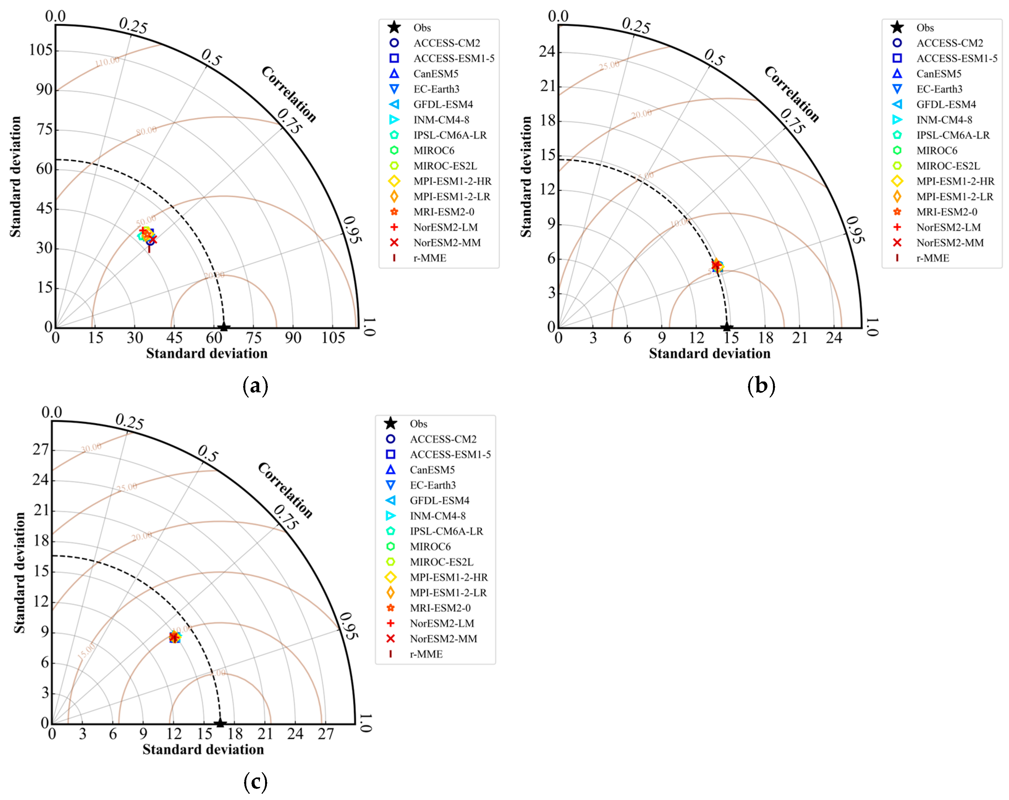
The data for the SWAT model and the CMIP6 global climate model under future climate scenarios are summarized in Table 1 and Table 2. The SWAT model data include the digital elevation model (DEM) of the lower Songhua River Basin, 2010 land use data, soil data, as well as daily data (1970–2014) from eight meteorological stations within the basin (including maximum and minimum temperatures, precipitation, relative humidity, and wind speed) and monthly runoff measurements (2000–2018) from the Jiamusi hydrological station. For the CMIP6 global climate model data, five of the most optimal climate models were selected from fourteen CMIP6 models using a Taylor diagram, and the data include three scenarios: SSP1-2.6, SSP2-4.5, and SSP5-8.5.

3. Methodology

3.1. Research Framework

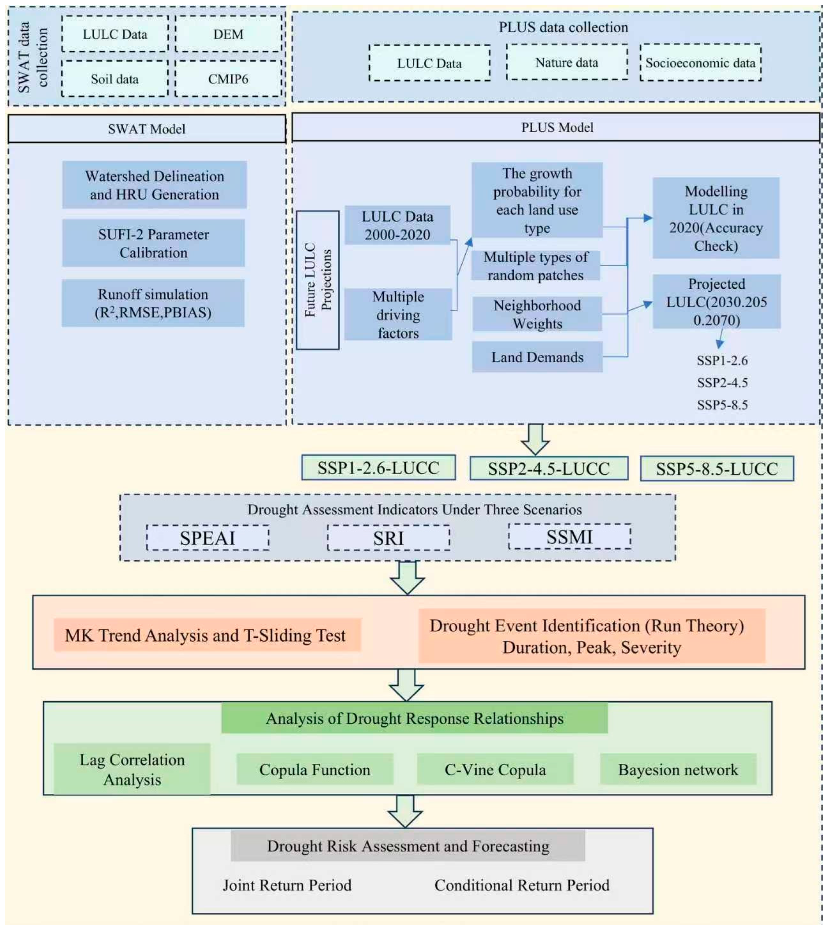
This study establishes an integrated methodological framework to investigate the evolution and propagation mechanisms of drought under future climate change scenarios. The framework sequentially employs: (1) SWAT hydrological model simulations calibrated using the SUFI-2 algorithm to model watershed processes; (2) PLUS model projections of future land-use patterns; (3) Climate projections derived from the Taylor plot-screened CMIP6 multi-model ensemble mean optimal (MMM-Best) ensemble; (4) Multiple drought indices (SPAEI, SRI, SSMI) combined with range theory to characterize meteorological, hydrological, and agricultural droughts; (5) Mann–Kendall trend analysis, Pettitt breakpoint tests, and lag correlation analysis to detect temporal dynamics and drought-response relationships; (6) Constructing nonlinear response models using copula-based methods (including C-Vine Copula and Bayesian networks) to quantify joint and conditional probabilities, determine propagation thresholds, and estimate multivariate recurrence intervals, thereby enabling a comprehensive assessment of drought risk characteristics and propagation pathways. The framework is illustrated in Figure 2.

3.2. SWAT Hydrological Model

3.2.1. Introduction to the SWAT Model and Simulation Methods

The SWAT model is a semi-distributed watershed hydrological model developed by the United States Department of Agriculture (USDA) [14,15,16]. Its primary purpose is to serve as a key tool for addressing hydrological, ecological, and environmental challenges in watersheds, and for simulating and predicting the impacts of land use changes on water quantity and quality [17,18]. The model has been extensively applied in research areas such as soil erosion, land use, and agricultural management [19]. A notable advantage of the SWAT model is the use of hydrological response units (HRUs) instead of raster-based calculations, which significantly reduces the computational load compared to other models. This feature makes SWAT highly effective for simulating large-scale watersheds over extended time periods. The simulation process involves: (1) delineating the study area, obtaining hydrological parameters based on the DEM, generating the river network, and subdividing the watershed into sub-watersheds; (2) overlaying and analyzing soil characteristics, land use, and watershed slope data to construct a comprehensive database, subdividing the sub-watersheds into multiple HRUs; and (3) calculating the runoff from each HRU to summarize the total river runoff [20]. The water balance equations used in the SWAT model are as follows:
S W t = S W 0 + i = 1 n ( R d a y Q s u r f E α W s e e p Q g w )
where S W t is the soil water content at the end of the period (mm); S W 0 is the soil water content at the beginning of the period (mm); t is the time step (day); R d a y is the amount of precipitation (mm); Q s u r f is the surface runoff (mm); E α is the evapotranspiration (mm); W s e e p is the lateral flux and infiltration in the stratum of the soil slope (mm); and Q g w is the groundwater content (mm).

3.2.2. SWAT Model Calibration

SUFI-2 (Sequential Uncertainty Fitting version 2) is one of the most widely used methods for uncertainty analysis and parameter calibration within the SWAT-CUP tool [21,22]. This method optimizes parameter ranges through iterative processes to minimize simulation errors and quantify the uncertainty of the simulation results. The core principle of SUFI-2 is to generate a large number of parameter combinations, based on a given parameter uncertainty, using the Monte Carlo method. The model is then run multiple times, and the strengths and weaknesses of the simulation results are evaluated using an objective function. After each iteration, the parameter ranges are updated according to the fit between the simulations and the observed data, gradually converging toward the optimal parameter space [23,24,25].
The model applicability evaluation adopts the goodness of fit coefficient R2, the Nash efficiency coefficient NSE and the percentage deviation PBIAS as the evaluation criteria [26], R2 and NSE indicate the degree of fit of the simulated values to the measured values, and PBIAS is used to measure the average trend of the simulated values to the observed values, and the formulas of the calculation method of the objective function and evaluation indexes as well as the evaluation criteria are as follows:
R 2 = i = 1 n Q 0 , i Q avg Q p , i Q pavg 2 i = 1 n Q 0 , i Q avg 2 i = 1 n Q p , i Q pavg 2
N S E = 1 i = 1 n Q Q , i Q p , i 2 i = 1 n Q Q , i Q a v g 2
P B I A S = 100 × i = 1 n Q o , i Q p , i i = 1 n Q 0 , i
where Q o , i , Q p , i , Q a v g , Q p a v g are measured flow, measured mean flow and simulated mean flow. When R2 and NSE are greater than 0.6 and 0.5, respectively, and the closer PBIAS is to 0, it indicates that the model is applicable to the watershed.

3.3. PULS Model

This study employs the PLUS model, which excels in deeply analyzing land use changes across various land types, enabling more accurate simulation of complex, multi-class land use evolution processes [27]. The PLUS model is a new-generation, high-precision land use change simulation model primarily used to simulate the spatiotemporal evolution of land use patterns under different scenarios. The model integrates the strengths of machine learning and geographic process modeling and consists of two core modules [28]: (1) LEAS (Land Expansion Analysis Strategy): Utilizing machine learning algorithms such as random forests, this module identifies the driving factors of land use change and predicts the probability of new land development. (2) CARS (CA based on Multi-type Random Seeds): A cellular automata module based on multi-type random seeds and an adaptive neighborhood mechanism, used for generating and evolving spatial patterns. Compared to traditional land use models (e.g., CLUE-S, CA-Markov), the PLUS model offers several advantages: it can generate patch-level spatial patterns, enhancing the realism of spatial simulations; supports multi-scenario modeling and scenario-driven analyses (e.g., ecological protection priority, urban expansion, SSPs-RCPs scenarios); improves the model’s capability in dynamic expansion and detailed spatial representation; and is suitable for research frameworks coupling climate change and land use change [29].
By considering factors such as correlation, timeliness, adaptability, policy, and economic aspects, this study selects 13 data items as driving factors for land use change (Refer to Supplementary Table S1). Based on land use data from 2000 and 2010, the expansion areas of various land use types are extracted. Using a random forest algorithm for sampling and computation, the development probabilities of different land use types are obtained. Combined with mechanisms such as the transition cost matrix and neighborhood weights, the spatial distribution of each land use type is reasonably predicted [30].
Neighborhood weights and the cost matrix are fundamental parameters for simulating the future spatial distribution of land use. The neighborhood weights are associated with land use types and must be determined based on the objective changes observed in the historical scenarios of the study area. The calculation formula is as follows:
W i = Δ T A i Δ T A min Δ T A max Δ T A min
In the formula, W i represents the neighborhood weight coefficient for a certain land use type i; T A i represents the area change of land type i during the study period; T A m a x and T A m i n , respectively, represent the maximum and minimum area changes during the study period.
The cost matrix depends on different land use scenarios set for the future. Based on relevant scenario data, the neighborhood weights for different land use types and the transition cost matrices under three scenarios are established (refer to Supplementary Table S2).
The model’s accuracy is assessed using the Kappa coefficient, overall accuracy (OA) and tests for quantity disagreement (QD) and allocation disagreement (AD). This approach reveals changes in spatial landscape information and is suitable for evaluating the similarity between two maps. The calculation formula is as follows:
K a p p a   = P o P c P p P c
O A = i = 1 k n i i N
Q D = i = 1 k p i r i 2
A D = D Q D
D = 1 O A
where P o is the percentage of simulated correct rasters, P p is the percentage of simulated correctness in the ideal state, P c is the percentage of simulated correctness in the random state, n i i denotes the element at the i-th row and i-th column of the confusion matrix (diagonal element), k represents the total number of categories, N represents the total sample size (number of all pixels), p i represents the proportion of category i in the prediction map, r i denotes the proportion of category i in the reference map, D stands for Total Disagreement.

3.4. CMIP6 Data Processing

CMIP6 models were ranked to identify the most suitable climate models capable of generating the most plausible future climate scenarios for the basin, which could then be applied to runoff and hydrological drought projections [31]. The Taylor diagram is a widely used and robust tool for ranking CMIP6 models due to its effectiveness in assessing the relative strength of competing models and evaluating overall performance as models evolve [32]. It integrates three statistical metrics: correlation (r), root mean square error (RMSE), and spatial standard deviation ratio (SD), which together provide insights into the degree of pattern correspondence [33]. In this study, the 14 CMIP6 climate models and the ensemble means of the top 5 models were compared with observed data from the Lower Songhua River (1970–2014) using Taylor diagrams. The results, shown in Figure 3, indicated that Tmax exhibited a high positive correlation (r > 0.92) and a low RMSE (<5.19) across all 14 climate models, while Tmin similarly showed a high positive correlation (r > 0.82). Additionally, the standard deviation ranges for Tmax were found to be between 14.74 and 14.95, and for Tmin, between 10.09 and 10.38. These findings suggest that all CMIP6 models are capable of predicting future temperatures in the watershed.
For precipitation prediction, all models performed well, but only five models demonstrated high correlation (r > 0.7), RMSE < 43.13, and a standard deviation of observations (<49.85). These models include MIROC-ES2L, ACCESS-ESM1-5, MPI-ESM1-2-HR, NorESM2-MM, and INM-CM4-8. Therefore, these five climate models were selected for pooled averaging. The optimal model, Multi-Model Mean-Best (MMM-Best), was derived, showing the highest correlation (r = 0.77), the smallest RMSE, and a high similarity to the observed data’s standard deviation (46.39). Consequently, the r-MME climate model was selected for studying future runoff and hydrological drought in the Lower Songhua River Basin from 2015 to 2100.

3.5. Drought Evaluation

3.5.1. Standardized Precipitation Actual Evapotranspiration Index

The study employs the Standardized Precipitation Actual Evapotranspiration Index (SPAEI) to assess meteorological drought. Compared to the Standardized Precipitation Evapotranspiration Index (SPEI), the primary advantage of SAPEI lies in its use of actual evapotranspiration, which more accurately reflects surface water conditions. This makes it particularly suitable for drought detection in hydrologically complex and drought-sensitive regions, such as agricultural irrigation areas. The calculation of meteorological drought in this study is based on actual evapotranspiration (ATE) and precipitation data derived from the SWAT model outputs [34]. The calculation formula is as follows:
E T A = 0.408 Δ ( R n G ) + Υ 900 T m e a n + 273 u 2 ( e s e a ) Δ + Υ ( 1 + 0.34 u 2 )
In the formula E T A denotes the actual monthly evapotranspiration of the region, Δ represents the slope of the saturated vapor pressure curve, R n denotes net surface radiation, G represents the soil heat flux, which can be neglected when the calculation timescale is monthly, Υ is the psychrometer constant, T m e a n represents the monthly average temperature, take the average of the daily maximum and minimum temperatures. u 2 is the wind speed at a height of 2 m, e a is the actual vapor pressure, e a is the saturated vapor pressure, T i represents the monthly average temperature, denotes the annual heat index.
Calculate the difference D i between the monthly precipitation ( P i ) and the actual evapotranspiration ( E T A ).
D i = P i E T A
Process data D i and calculate the corresponding SPAEI index using a log-logistic probability distribution, with the formula as follows:
F ( x ) = 1 + α x γ β 1
Standardization of cumulative probability density:
P = 1 F ( x )
When the cumulative probability is P ≤ 0.5:
W = 2 ln ( P )
S P E A I = W c 0 + c 1 W + c 2 W 2 1 + d 1 W + d 2 W 2 + d 3 W 3
In the formula c 0 = 2.515517, c 1 = 0.802853, c 2 = 0.010328, d 1 = 1.432788, d 2 = 0.189269, d 3 = 0.001308.
When P > 0.5 is true, the value of P is taken as 1-P:
S P E A I = W + c 0 + c 1 W + c 2 W 2 1 + d 1 W + d 2 W 2 + d 3 W 3

3.5.2. Standardized Runoff Index and Standardized Soil Moisture Index

This study employs the Standardized Precipitation Evapotranspiration Index (SPAEI), Standardized Runoff Index (SRI), and Standardized Soil Moisture Index (SSMI) to characterize meteorological drought, hydrological drought, and agricultural drought, respectively. These indices are widely applied in hydrological and meteorological watershed studies. Generally, seasonal-scale drought indices are more suitable for identifying continuous drought events in watersheds. Therefore, this study constructs response relationships between meteorological–hydrological and meteorological–agricultural droughts based on SPAEI-3, SRI-3, and SSMI-3 [34]. According to the national standard Meteorological Drought Grades: GB/T 20481—2017 [35], drought indices are classified into five levels, as shown in Table 3. The calculation formulas for SRI and SSMI are as follows:
F ( x ) = 0 x x α 1 β α Γ e x β d x
In the formula α is the shape parameter, β is the scale parameter, and all parameters are real numbers greater than zero.
The formula for calculating W in SRI differs from the aforementioned SPEAI calculation, but ultimately converges with the formula for the drought index. The formula for calculating W is as follows:
W = ln 1 F ( x ) 2
The formula for calculating the Agricultural Drought Index (SSMI) is as follows
S S M I i , j = S M i , j S M j ¯ j
Here, i denotes the observation year, j represents the observation month from January to December, while S M j and j denote the mean and standard deviation of soil moisture for the jth month, respectively. The dimensionless SSMI value is used to monitor drought conditions: when SSMI exceeds 0, it indicates that the soil moisture for that month is above the long-term average for the same period; conversely, it indicates drought.

3.5.3. Run Theory

Run Theory has been extensively studied in the identification and characterisation of drought events, and the process of Run Theory identification mainly focuses on effective data compression by traversing the data and identifying subsequences of consecutive identical elements (runs). It is used not only for data compression but also for pattern recognition, signal processing and other fields [36]. The main identification processes are (1) Initial identification of drought months. Setting the theoretical identification of drought indicator thresholds R 0 = 0 , R 1 = 0.3 , R 2 = 0.5 , when the SSI is less than R 1 , it can initially be considered as a drought; (2) the elimination of small drought time. If a drought event lasts only one month, the SSI is greater than R 2 , which is considered a small drought event and is excluded from the statistics; (3) merging of drought events. If two drought events are separated by only one month and the SSI is less than R 0 , they are combined into one drought event [37].

3.6. M-K Trend Analysis and Pettitt Mutation Test

The nonparametric Mann–Kendall (M-K) test and Pettitt abrupt change analysis, widely employed in trend analysis of meteorological and hydrological time series, were utilized to reveal shifts in future drought evolution trends and abrupt change time points. For specific formula steps, refer to the literature [38].

3.7. Lag Correlation

Lag correlation refers to the correlation between two time series under a specific time lag. In this study, for each possible lag k (k = 1, 2,…, 12 months), the meteorological drought series is kept stationary, while the hydrological drought series and agricultural drought series are shifted backward by k time steps (i.e., hydrological and agricultural droughts occur k months after the meteorological drought). The Spearman rank correlation coefficient is then calculated for the shifted series combinations [39]. The calculation formula is:
ρ k = 1 6 t = 1 n k d t 2 n n 2 1
In the formula d t = R X t R Y t + k is the rank difference between X t and Y t + k at time t, n is the length of the time series.

3.8. A Joint Analysis Method for Drought Events Based on Copula Functions

3.8.1. Nonlinear Response Model Based on Copula Functions

The drought response models are mainly divided into linear and nonlinear function models. Generally, linear functions are used to reflect the relationships between drought characteristic variables and are widely applied in constructing response models for drought characteristic variables. Nonlinear functions, on the other hand, can effectively fit the relationships, transmission time, and thresholds between drought characteristic variables, finding certain applications in constructing models for different drought types [40].
The Copula function, proposed by Sklar et al. [41] in 1959, is a multivariate joint distribution function with results uniformly distributed in [0, 1]. First, marginal distributions of two or more correlated variables are constructed, and then the Copula function is used to build their joint distribution. According to Hao et al., the conditional probability based on the Copula function can be used to establish nonlinear relationships between variables and for probabilistic forecasting [42]. Drawing on this approach, this study establishes nonlinear response models between the meteorological drought characteristic variable X and the hydrological drought characteristic variable Y, as well as between the meteorological drought characteristic variable X and the agricultural drought characteristic variable Z, to derive the conditional probability distribution of Y in response to X. F x ( x ) , F y y , F z ( z ) are the marginal distribution functions for the variables X and Y, respectively. Let u = F x ( x ) , v = F y y ,   w = F z ( z ) , The joint distribution function and probability density function of X and Y are, respectively:
F ( x , y ) = C F x ( x ) , F y ( y ) = C ( u , v )
f ( x , y ) = C ( u , v ) f x ( x ) f y ( y )
In the formula C ( u , v ) is the Copula function representing the joint distribution function of X and Y; f x ( x )   f y ( y ) are the marginal probability density functions for the variables X and Y, respectively. Let X = x ; the conditional probability distribution function for the occurrence of variable Y is obtained as:
F y / x ( y ) = P ( Y y X = x ) =   F ( x , y ) / x d F x ( x ) / d x = C ( u , v ) u
The corresponding conditional probability density function is:
f Y / X ( y ) = f ( x , y ) / f X ( x ) = C ( u , v ) f Y ( y )
Let d f y / x ( y ) / d y = 0 The Y value corresponding to the maximum of the conditional probability density function can be obtained and used as the predicted value.
Similarly, the joint distribution function and probability density function of X and Z follow the same formulas as above.
The calculation formula for the three-dimensional joint distribution based on the Copula function is:
F ( x , y , z )   = P ( X x , Y y , Z z ) = C F X ( x ) , F Y ( y ) , F z ( z ) = C ( u , v , w )

3.8.2. C-Vine Copula Model

In recent years, bivariate Copula parametric models (Archimedean and elliptical Copulas) have been widely applied in hydrological variable analysis. LI et al. established a drought severity-area-frequency curve using Copula functions in China’s Heihe River Basin and assessed the curve’s uncertainty [43]. Esit, Musa et al. derived bivariate probability distributions for drought severity and duration based on Copula functions in Turkey’s Ceyhan Basin [44]. However, in high-dimensional cases, their simulation accuracy is reduced due to parameter constraints and computational complexity. In contrast, Vine Copula models based on hierarchical graphs outperform traditional single-parameter Copulas in multivariate hydrological data modeling. Vine Copulas can be categorized into C-Vine and D-Vine types [45]. Since the C-Vine Copula model is more suitable for scenarios with significant dominant dependency relationships among variables, this study primarily focuses on this model for multivariate simulation of drought characteristics. To quantitatively distinguish the impact of each variable on drought occurrence risk, the AND scenario is taken as an example:
P ( X x , Y y , Z z ) = 1 F X ( x ) F Y ( y ) F Z ( z ) + C F X ( x ) , F Y ( y ) + C F X ( x ) , F Z ( z ) + C F Y ( y ) , F Z ( z ) C F X ( x ) , F Y ( y ) , F Z ( z ) ] = 1 u v w + C ( u , v ) + C ( u , w ) + C ( v , w ) C ( u , v , w )
The meanings of the letters represented in the formula are consistent with those in Section 3.8.1.

3.8.3. Bayesian Network Probabilistic Model

The Bayesian network probability model effectively addresses uncertainty issues within a system by integrating conditional probability methods to estimate relationships between variables [46]. This study employs a first-order Bayesian network probability model for computation. In practical production and daily life, people are more concerned with the response probability of one variable or a pair of variables under specific conditions. Taking the conditional probability of mild (moderate or severe) agricultural drought occurring under mild (moderate or severe) meteorological drought conditions as an example, the calculation formula is:
P ( x 1 < X x 2 | y 1 < Y y 2 ) = C ( F X ( x 1 ) , F y ( y 2 ) ) + C ( F x ( x 1 ) , F y ( y 1 ) ) F y ( y 2 ) F y ( y 1 ) C ( F X ( x 1 ) , F y ( y 2 ) ) + C ( F x ( x 2 ) , F y ( y 1 ) ) F y ( y 2 ) F y ( y 1 )
In the formula X and Y represent SRI and SAPEI/SSMI, respectively. To further determine the triggering thresholds for different levels of hydrological and agricultural droughts under meteorological drought conditions, SAPEI is iterated from −0.5 with a step size of −0.1, and the corresponding probability P is calculated. A probability of 0.5 is set as the triggering threshold, i.e., when P ≥ 0.5, the iteration stops, and the value on the right side of the interval is taken as the transmission threshold.

3.8.4. Recurrence Interval and Recurrence Interval Under Copula Functions

The return period is a statistical indicator used in hydrometeorological research to characterize the frequency of extreme events. Following Chow’s (1951) classic definition, the return period T represents the average interval between events of a specific intensity or greater. For univariate cases, if X is a random variable representing drought characteristics (such as duration, intensity, or peak), the recurrence interval associated with threshold x0 is defined as:
T ( x 0 ) = 1 P ( X > x 0 ) = 1 1 F x ( x 0 )
Here, FX(x0) denotes the cumulative distribution function (CDF) of X at x0, while P(X > x0) represents the exceedance probability. In multivariate drought analysis based on Copula functions, this paper employs two return periods to characterize different risk scenarios: (1) The joint recurrence interval characterizes the average time interval during which all drought characteristics simultaneously exceed their respective thresholds. For a three-variable drought event comprising duration D, drought intensity S, and peak intensity P. (2) The return period, also known as the OR return period, represents the average time interval during which at least one drought characteristic exceeds its threshold. The formulas for calculating the two recurrence periods are as follows:
T A N D = 1 P ( D > d 0 S > s 0 P > p 0 )
T O R = 1 P ( D > d 0 S > s 0 P > p 0 )
According to the principle of inclusion-exclusion, this probability can be calculated as:
P ( D > d 0 S > s 0 P > p 0 ) = 1 P ( D d 0 S s 0 P p 0 ) = 1 C ( u 1 , u 2 , u 3 )
Here, C(·) denotes the copula function, and ui = Fi(xi) represents the CDF transformation of the marginal distribution. The return period is crucial for early warning systems as it identifies drought occurrences when any single variable reaches a critical state.

3.8.5. Model Accuracy Evaluation

The model simulation accuracy is evaluated using four indicators: the coefficient of determination (R2), root mean square error (RMSE), Akaike Information Criterion (AIC), and Bayesian Information Criterion (BIC). An R2 value close to 1 indicates a high correlation between the simulated results and actual values, while an R2 value close to 0 indicates a low correlation. Generally, smaller values of RMSE, AIC, and BIC indicate higher model accuracy [47].

4. Results and Analysis

4.1. SWAT Model Parameterisation and Validation

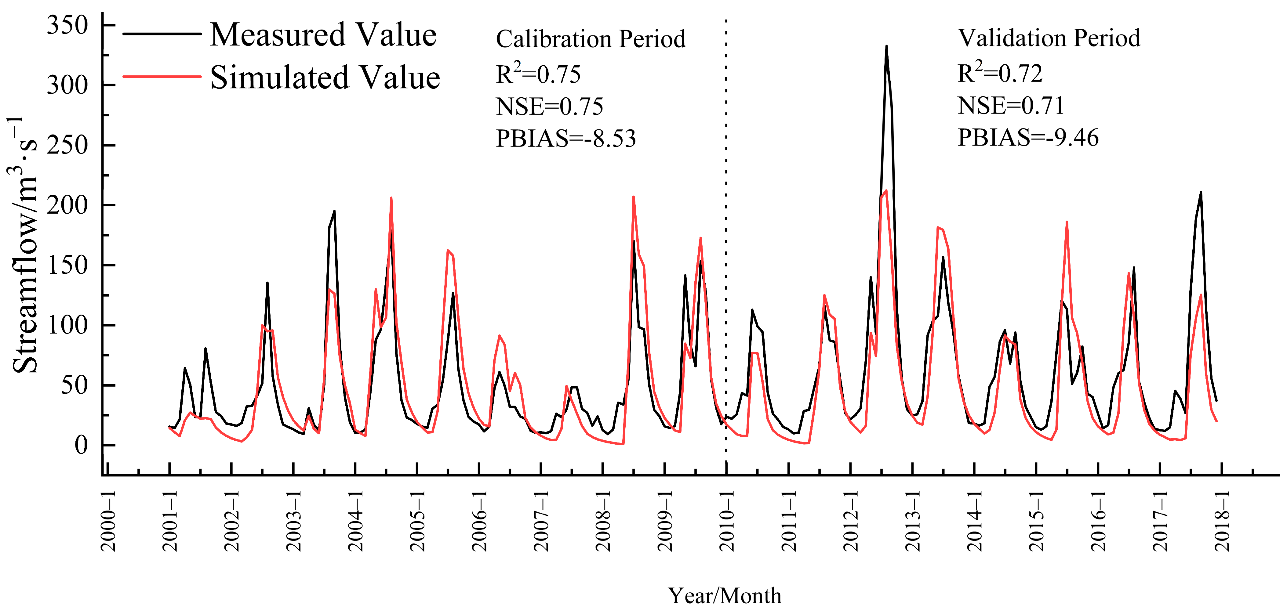
The measured runoff values from Jiamusi Hydrological Station were used to calibrate and validate the SWAT model, with parameter sensitivity analysis performed using the SWAT-CUP software (Version 5.1.6). The parameters with the most significant impact on the model’s simulation results were selected for calibration, and a total of 16 parameters were ranked based on their sensitivity to runoff in the watershed. The results are shown in Supplementary Table S3, where the periods 2000–2010 and 2011–2018 were used for calibration and validation, respectively. The fitting results for these two periods are presented in Figure 4. From Figure 3, it is evident that the monthly runoff simulations at Jiamusi Hydrological Station align well with the measured values, with the calibration and validation periods yielding the following indicators: R2 = 0.75, 0.72; NSE = 0.75, 0.71; and PBIAS = −2.4, −3.5, respectively. Based on the PBIAS, it is noted that runoff is slightly underestimated during both the calibration and validation periods. The underestimation could result from the further optimisation of SWAT parameters, particularly those relating to runoff generation and flow routing. Additionally, the accuracy of the model may be affected by changes in land use, given that the land use and soil data are from 2010, whereas the meteorological data span the period from 1970 to 2014. Nevertheless, the model demonstrates significant potential for predicting runoff under future climate scenarios in the Lower Songhua River Basin.

4.2. Land Use

Land use changes from 2000 to 2020 are illustrated in the Sankey diagram in Supplementary Figure S1. In the lower reaches of the Songhua River Basin, cropland, forestland, grassland, and unused land decreased by 371.22, 28.21, 0.04, and 3.49 km2, respectively, while water areas and urban land increased by 48.43 and 354.54 km2, respectively.

4.3. Analysis of the Driving Forces of Cultivated Land, Forest Land and Construction Land

In ArcGIS software (10.8.2), the land use data for the starting and ending years were reclassified, with six land classes assigned values ranging from 1 to 6, respectively. The reclassified land use data for 2000 and 2020 were then imported into the PLUS model to analyze the driving forces behind the changes in the three land classes in the Lower Songhua River Basin. The results are presented in Supplementary Figures S2 and S3. Figure S2 reveals that different land-use types are governed by fundamentally distinct driving mechanisms. Urban areas expansion is primarily controlled by topographic accessibility and proximity to administrative centers, reflecting socioeconomic development patterns. Cropland distribution, conversely, is determined almost entirely by natural conditions (DEM and precipitation), indicating that cropland land allocation is constrained by environmental factors rather than economic development. Forest distribution exhibits a mixed pattern, influenced by both natural factors (temperature, DEM) and human activities (nighttime lights), suggesting that forest extent results from the interplay of environmental suitability. Figure S3 reveals three critical transformation hotspots: (1) concentrated cropland decline in the central and southern regions (shown in red), primarily converting to urban areas associated with urban expansion; (2) newly developed urban areas (marked in red) predominantly located in the northern and central parts of the basin, following major transportation corridors; and (3) localized forest cover reduction (marked in red) in the eastern mountainous areas, corresponding to agricultural expansion and development activities.

4.4. Multi-Scenario Simulation of Land Use

Using the year 2000 as the base year, spatial distribution was predicted based on the PLUS model, yielding a Kappa coefficient of 0.83, an OA of 92.85%, a QD of 5.70%, and an AD of 1.44%. Subsequently, the rate of land area change in the Lower Songhua River Basin was analyzed for the short-term (2020–2030), medium-term (2020–2050), and long-term (2020–2070) periods. In the SSP1-2.6 scenario, a dramatic increase in grassland area, a slight decrease in arable land and bare land, and a small increase in construction land are observed. This is due to the emphasis on resource conservation and ecological restoration in this scenario, which drives land use changes towards more sustainable and ecologically friendly practices. In the SSP2-4.5 scenario, grassland continues to expand, arable land shrinks, and construction land grows slowly. This reflects a “natural evolutionary” development mode, with moderate land use changes and urban expansion gradually encroaching on arable land, but limited ecological restoration measures. In the SSP5-8.5 scenario, grassland remains the dominant land use type, with continued decline in arable land and an acceleration in construction land expansion. This scenario reflects an economic development path that prioritizes economic growth at the expense of ecological values, leading to significant urban expansion pressure and land degradation trends, which may exacerbate environmental vulnerability in the future [48].

4.5. Temporal Evolution Characteristics and Abrupt Changes of Drought Indices Under Different SSP Scenarios

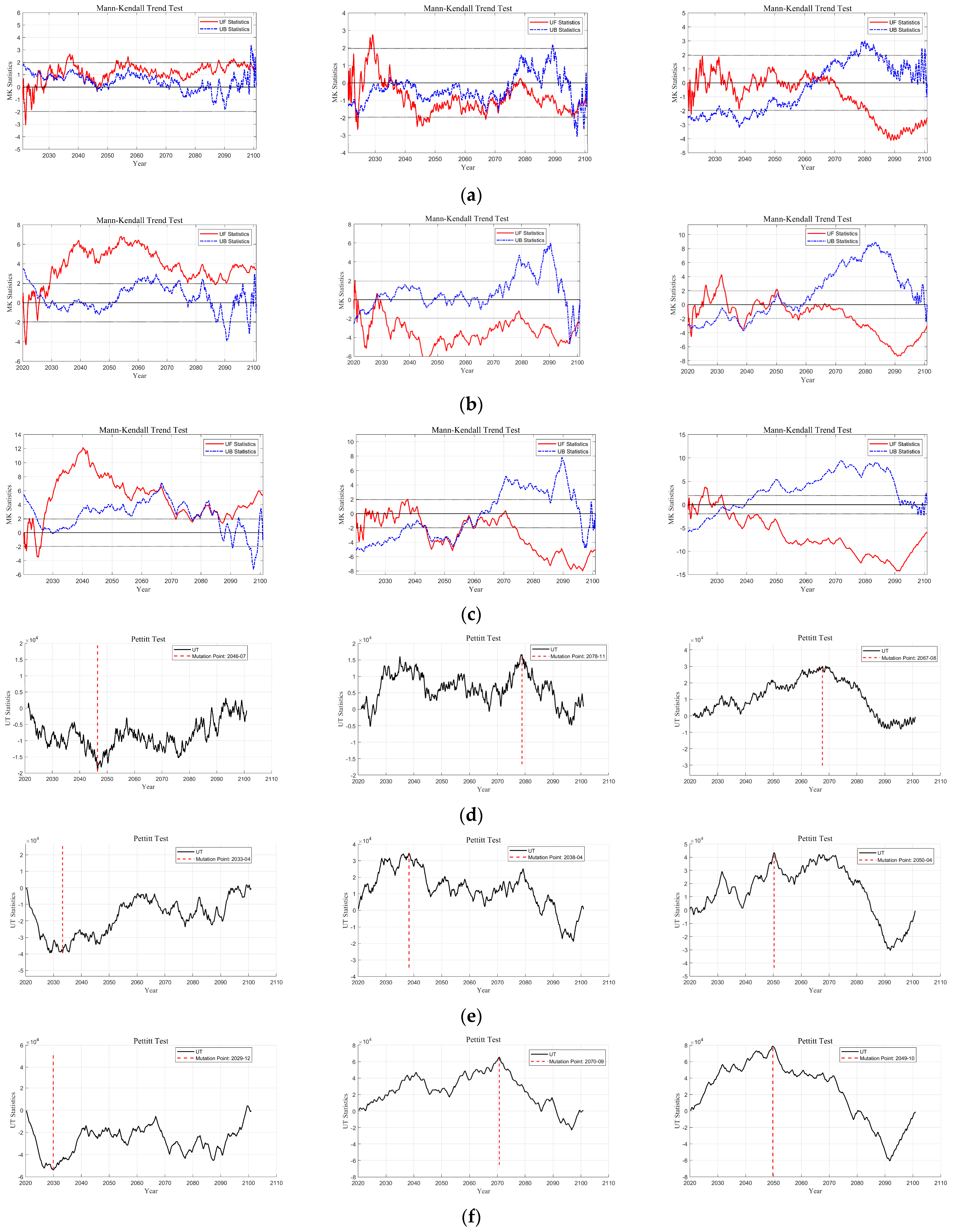
To reveal the temporal evolution patterns of drought indices under different land-use scenarios, this study analyzed the SPEI, SRI, and SSMI indices across three SSP scenarios using the Mann–Kendall trend test and Pettitt change test.
As shown in Figure 5, the Mann–Kendall test indicates significant differences among the three scenarios. Under the SSP1-2.6 scenario, SPEI remains relatively stable while SRI and SSMI exhibit extremely significant upward trends. The UF statistic peaks at +7.0 in 2060 and +12.0 in 2040–2045, reflecting substantial improvements in runoff and soil moisture under sustainable development. Under SSP2-4.5, SPEI remained within the ±2.0 significance threshold, while SRI reached high values of +5.0 to +6.0 between 2060 and 2080. SSMI declined to approximately −3.0 by the end of the century, indicating pressure on soil moisture. Under the SSP5-8.5 scenario, SPEI and SRI both reach +3.0 after 2070, while SSMI exhibits a rare opposite pattern of UF and UB statistics (UF drops to −4.0, UB rises to +3.0), reflecting extremely high uncertainty under this high-intensity scenario.
The Pettitt mutation test identified critical mutation points. Under the SSP1-2.6 scenario, mutation points clustered between 2029 and 2046 (UT: 19,500–52,000), while those under SSP2-4.5 occurred between 2038 and 2070 (UT: 30,000–65,000). Meanwhile the SSP5-8.5 scenario concentrated between 2049 and 2050 (UT: 43,000–78,000), with SRI reaching its peak mutation intensity. Scenario comparisons reveal: - Temporal dimension: SSP1-2.6 exhibits earliest changes (2025–2035), SSP2-4.5 shows gradual transitions (2038–2078), and SSP5-8.5 demonstrates concentrated abrupt shifts (2049–2050). In terms of index sensitivity, SPEI exhibits the most conservative response, SRI shows the strongest response under high-intensity scenarios, and SSMI demonstrates the highest sensitivity. Regarding abruptness intensity, the UT statistic increases systematically from SSP1-2.6 to SSP5-8.5, with SRI showing an increase exceeding 240%.

4.6. Probability of Combined Occurrence of Drought Under the Condition of Different Combinations of Characteristic Variables

4.6.1. Marginal Distribution of Drought Characteristics and Copula Function Construction

This study identifies drought events based on operational theory, yielding frequency and average characteristics for meteorological, hydrological, and agricultural droughts, as shown in Table S4 of the Supplementary Materials.
The AIC test results for the fitted distributions of drought duration, drought intensity, and peak drought intensity for different drought types in the lower reaches of the Songhua River basin under three SSP scenarios for the periods 2020–2060 and 2061–2100 are presented in Supplementary Tables S5–S7. The distribution corresponding to the minimum AIC value was selected as the optimal fitted distribution for a given drought characteristic variable, i.e., the marginal distribution [49].
Supplementary Tables S8–S16 present the optimal linking functions for various drought characteristic variable combinations in the lower Songhua River basin under three SSP scenarios for the periods 2020–2060 and 2061–2100. These parameters were determined based on AIC, BIC, RMSE, and K-S criteria. The selection of optimal linking functions is based on the following criteria: achieving a K-S test significance level of 0.05 while simultaneously minimizing AIC and BIC values and minimizing RMSE.
Supplementary Figures S6–S8 illustrate the relationship between empirical frequency and theoretical frequency for the optimal Copula function of multidimensional drought characteristic variables under three drought types. As shown in Figures S6–S8, both theoretical and empirical frequencies exhibit good consistency across the three drought types in all three scenarios, indicating that the results from the optimal Copula function are reasonable and reliable.

4.6.2. Probability of Combined Occurrence of Two-Dimensional Drought

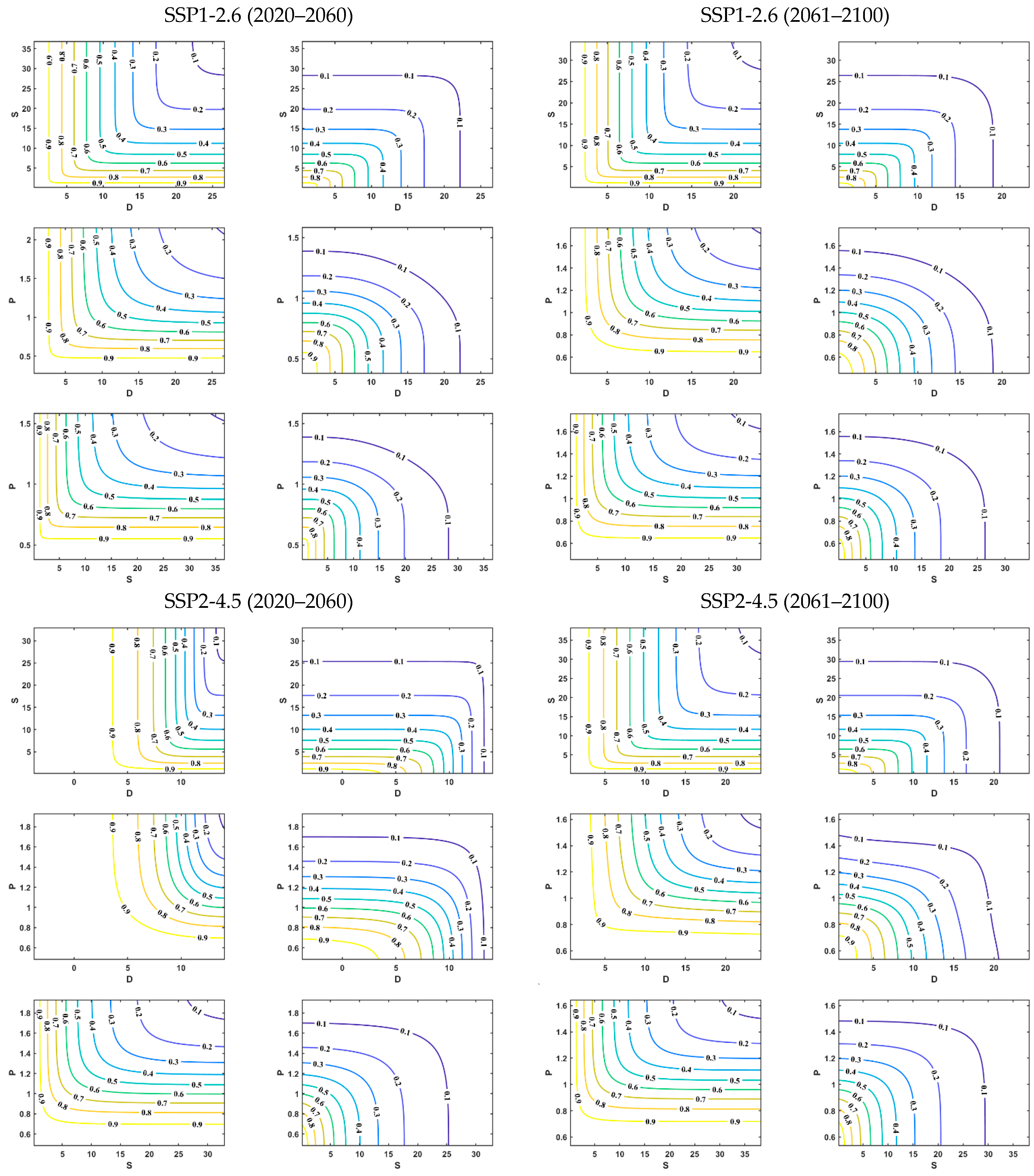
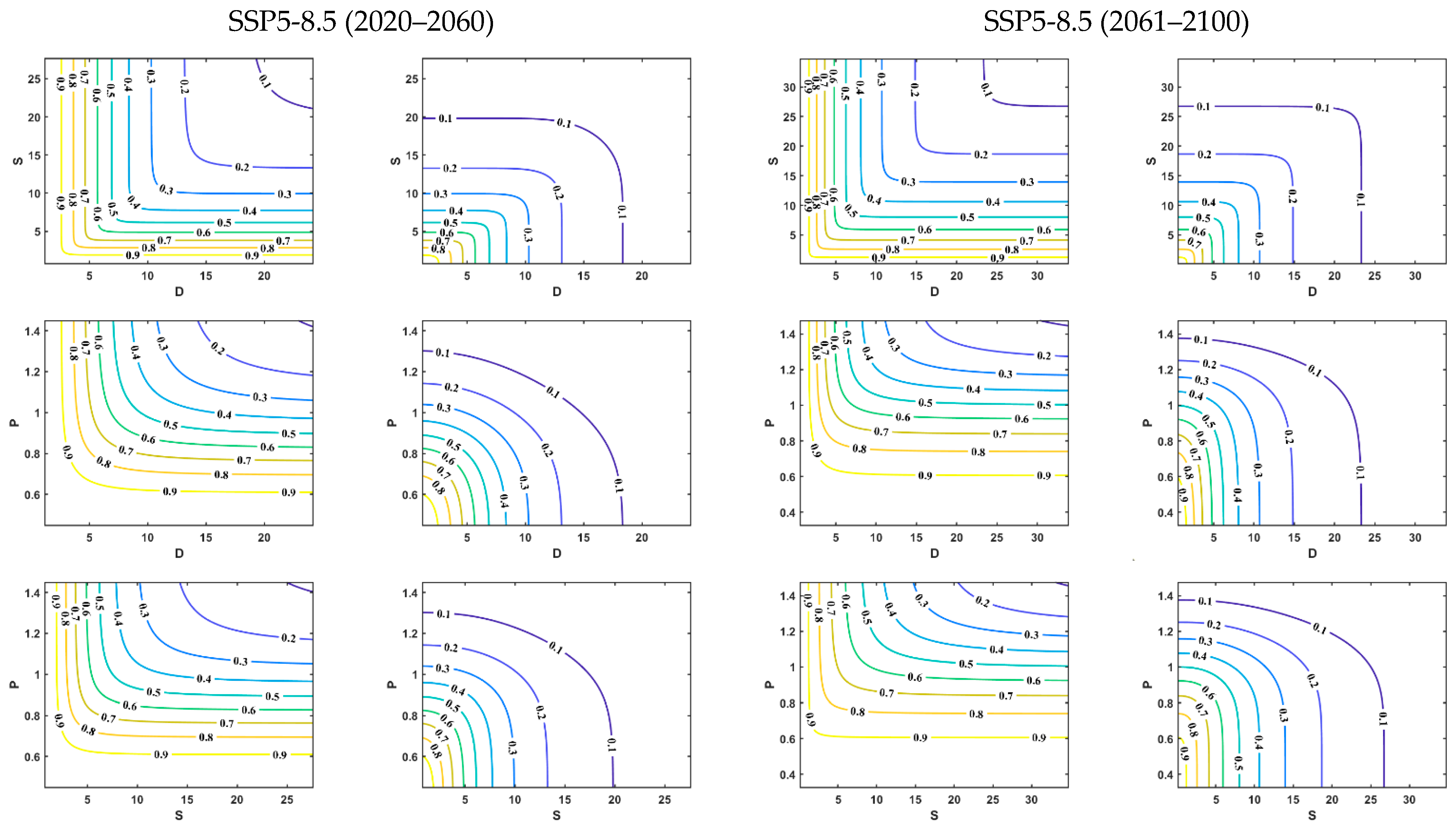
Figure 6 displays the bivariate joint probability distributions for meteorological drought characteristics in the lower Songhua River basin (D-S, D-P, and S-P). The joint occurrence probability is inversely proportional to the magnitude of drought characteristics. Under both “OR” and “AND” conditions, when one characteristic remains constant, the probability decreases as the other characteristic increases. Similar trends are observed in the hydrological and agricultural drought patterns (Supplementary Figures S6 and S7).
Drought characteristics for 2020–2100 are ranked by frequency, with cumulative distribution thresholds of 75%, 50%, and 25% representing mild, moderate, and severe droughts, respectively (Table 4). Under the SSP1-2.6 scenario, meteorological droughts in the D-S combination showed a decreasing trend from 2061 to 2100 compared to 2020–2060, with the largest reduction occurring at the 50% threshold (P_OR: −0.07, P_AND: −0.05). The D-P combination exhibited mixed trends: changes at the 75%, 50%, and 25% thresholds were (+0.06, +0.05), (+0.11, −0.04), and (−0.01, +0.02), respectively. The S-P combination primarily increased, with the most significant change occurring at the 50% level. Under the SSP2-4.5 scenario, D-S and D-P showed the greatest change at the 25% level, while S-P peaked at the 50% level. Under the SSP5-8.5 scenario, D-S peaked at the 75% level, and D-P and S-P peaked at the 25% level.
The hydrological drought pattern under SSP1-2.6 resembles the meteorological drought pattern under SSP5-8.5. Under SSP2-4.5, D-S exhibits the greatest change at the 75th percentile, while D-P and S-P peak at the 50th percentile. The SSP5-8.5 scenario exhibits consistent behavior across all combinations, with maximum changes occurring at the 75% percentile, indicating heightened sensitivity to mild drought under high radiative forcing.
Agricultural drought under the SSP1-2.6 scenario exhibits consistency, with all combinations showing maximum variation at the 50% threshold, indicating sensitivity to moderate drought under low radiative forcing. The SSP2-4.5 scenario reveals divergent patterns: D-S and D-P peak at the 75% threshold, while S-P peaks at the 50% threshold, suggesting differentiated responses to the medium-forcing scenario.

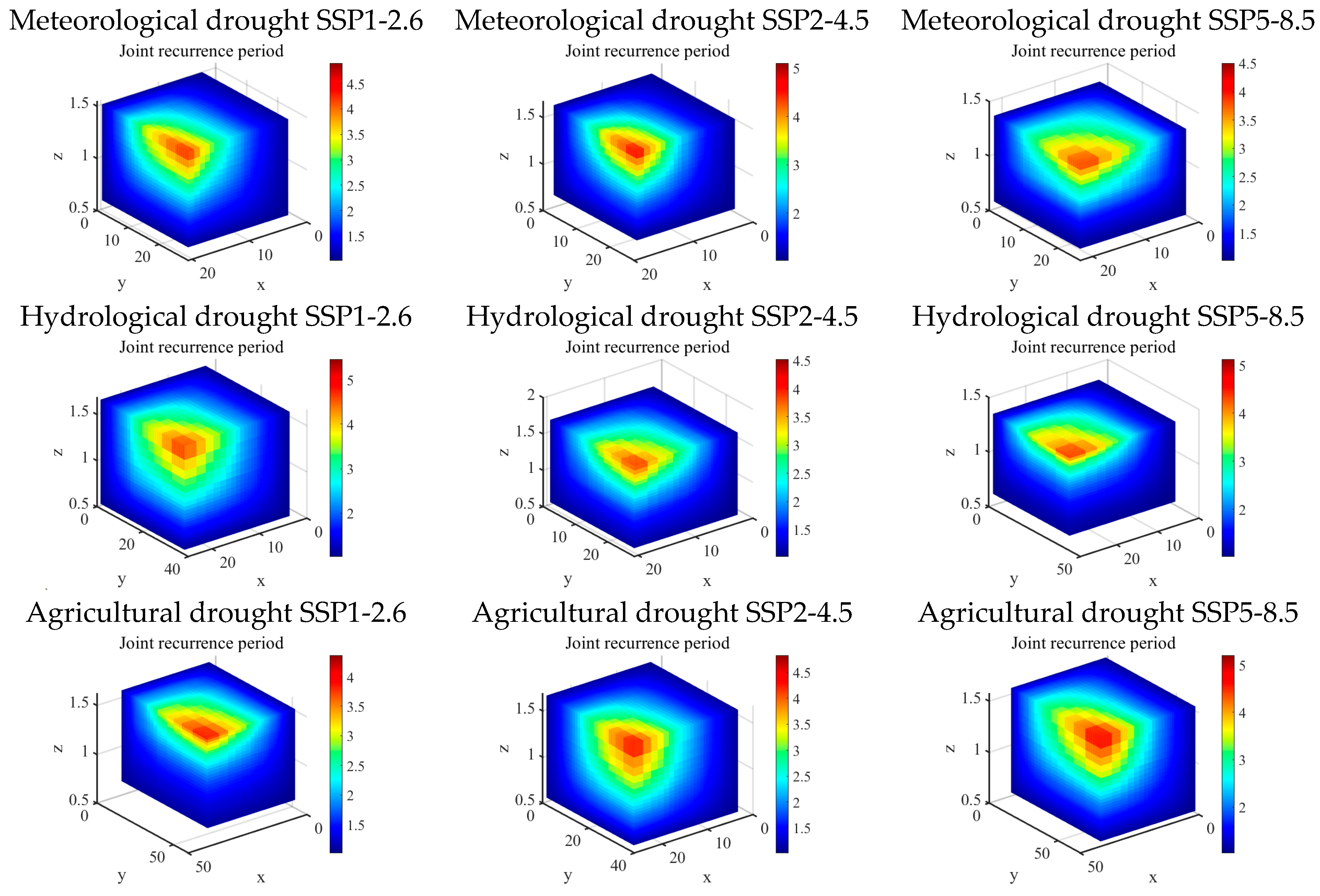
4.6.3. Probability of Combined Occurrence of Three-Dimensional Drought

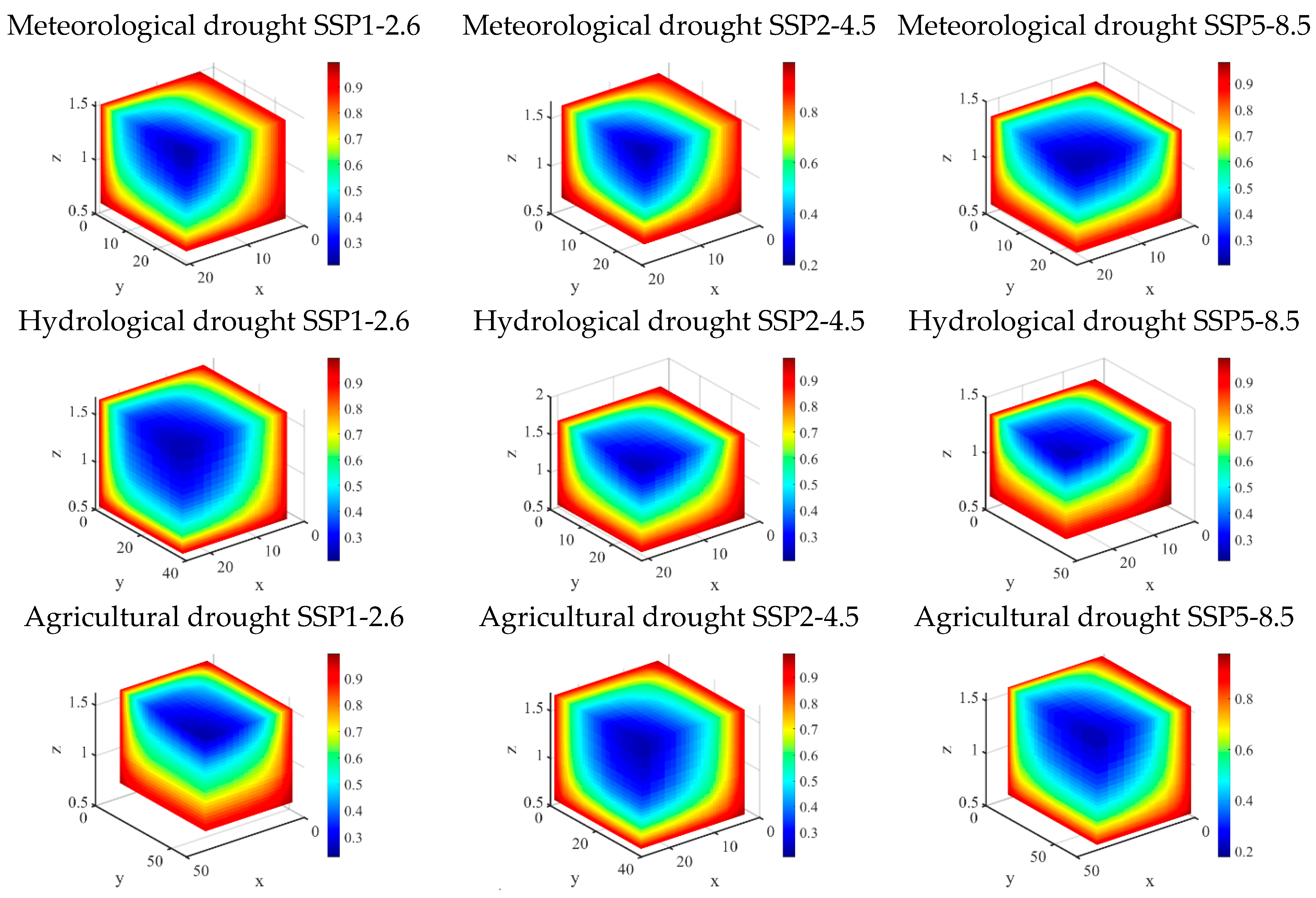
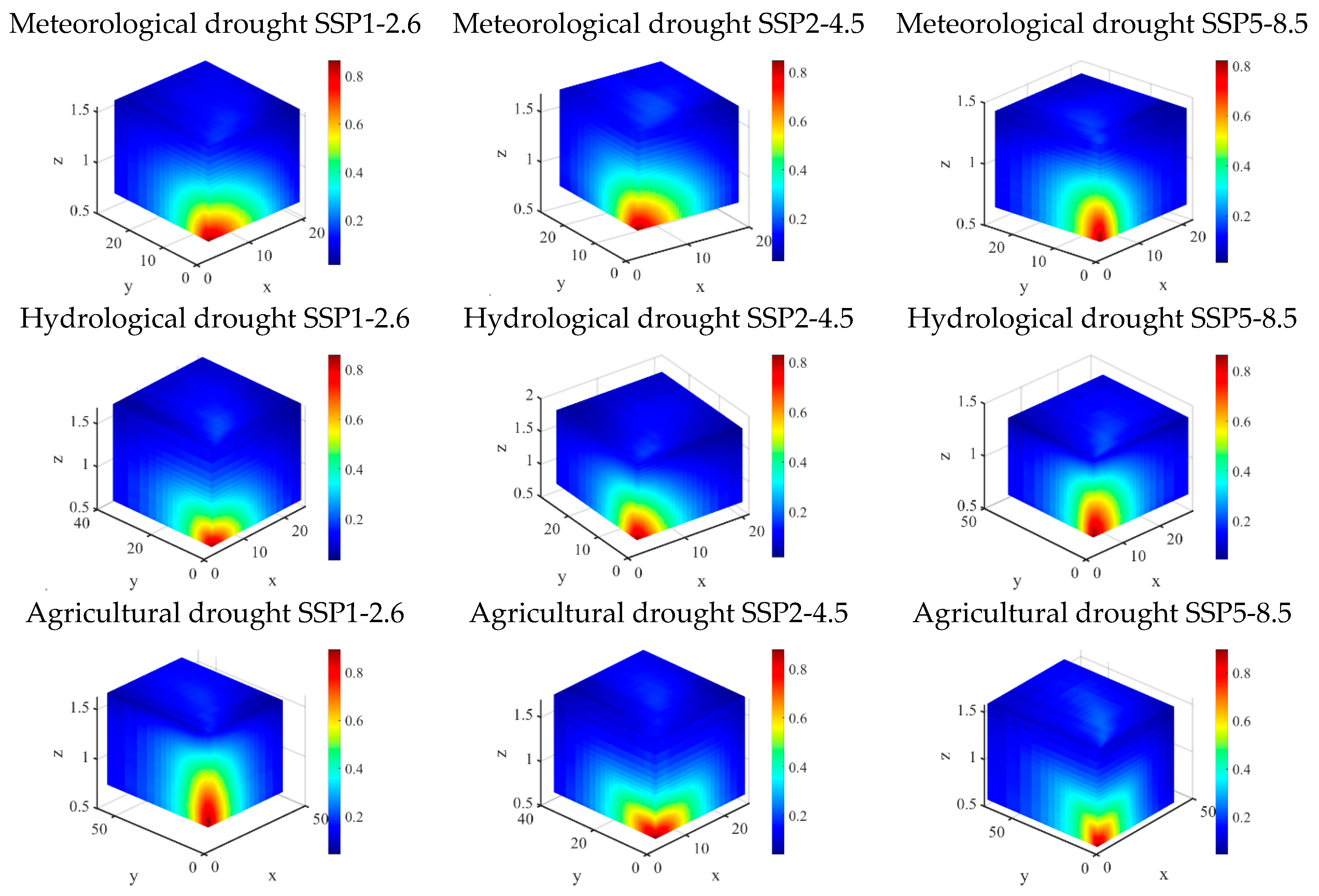
Figure 7 and Figure 8 display the three-dimensional joint probability distributions of meteorological drought under “or” and “and” conditions across multiple climate scenarios. The three-variable probability surfaces exhibit a monotonically decreasing trend with increasing drought severity, reflecting the inverse relationship between extreme events and their occurrence frequency [30]. For the three drought variables (D, S, P), under SSP1-2.6, SSP2-4.5, and SSP5-8.5 scenarios (2020–2100).
For meteorological drought, the P_oDSP and P_aDSP probabilities under the 75%, 50%, and 25% thresholds in the SSP1-2.6 scenario are (0.98, 0.73), (0.84, 0.45), and (0.48, 0.18), respectively. For SSP2-4.5, these values are (0.95, 0.66), (0.72, 0.36), and (0.53, 0.22), while SSP5-8.5 yields (0.96, 0.68), (0.80, 0.45), and (0.45, 0.19). SSP1-2.6 exhibited the highest probability during mild to moderate droughts, whereas SSP2-4.5 dominated at severe drought thresholds, indicating a non-monotonic relationship with radiative forcing pathways.
For hydrological drought, the probabilities at the 75%, 50%, and 25% thresholds are: SSP1-2.6 (0.96, 0.73), (0.79, 0.54), (0.49, 0.28); SSP2-4.5 (0.95, 0.63), (0.83, 0.43), (0.48, 0.18); SSP5-8.5 (0.97, 0.73), (0.82, 0.53), (0.47, 0.23). SSP5-8.5 exhibited the highest probability during mild to moderate droughts, while SSP1-2.6 became dominant during severe droughts, indicating distinct transmission mechanisms and water storage buffering effects across different climate scenarios.
For agricultural drought, the probabilities across scenarios are: SSP1-2.6 (0.97, 0.72), (0.87, 0.54), (0.53, 0.30); SSP2-4.5 (0.95, 0.79), (0.78, 0.60), (0.56, 0.38); SSP5-8.5 (0.98, 0.83), (0.77, 0.66), (0.37, 0.28). A tri-modal pattern emerges: SSP5-8.5 dominates during mild droughts, SSP1-2.6 peaks during moderate droughts, and SSP2-4.5 reaches its maximum at severe drought thresholds. This non-monotonic relationship reflects complex interactions between soil moisture, vegetation responses, and climatic variability, distinguishing agricultural drought from meteorological and hydrological drought patterns.

4.6.4. Two-Dimensional Recurrence Period

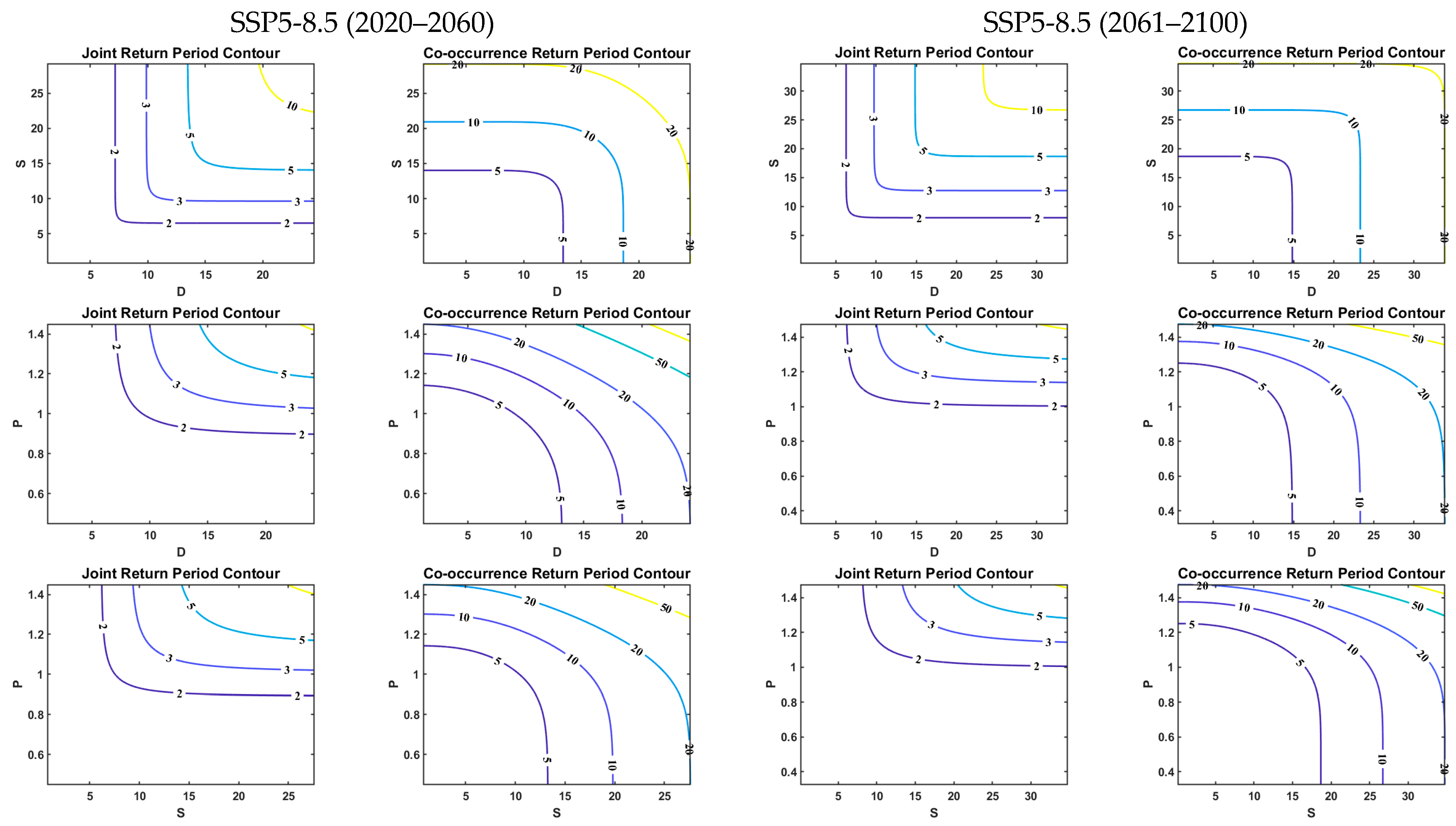
Figure 9 displays the bivariate return period distribution of meteorological drought characteristic combinations (D-S, D-P, S-P) across different scenarios and time periods in the lower reaches of the Songhua River basin. Return periods under the “and” condition consistently exceed those under the “or” condition. Spatially, this manifests as sparse and widely spaced ‘and’ condition isoclines, whereas “or” condition isoclines are densely clustered with narrow intervals. The maximum return periods are concentrated in the upper-right quadrant of the probability space, corresponding to scenarios where both drought characteristics simultaneously reach high values. Supplementary Figures S8 and S9 present similar analyses for hydrological and agricultural droughts, revealing spatiotemporal patterns consistent with meteorological drought. This indicates that drought signals propagate synergistically across the atmosphere–land–agriculture continuum.
Based on the joint distribution probability, droughts are characterized as mild, moderate, and severe using cumulative frequency thresholds of 75%, 50%, and 25%, respectively. Under the SSP1-2.6 scenario, the return periods for R-oDS and R-aDS at the 75%, 50%, and 25% thresholds for the D-S combination in 2061–2100 were (1.15, 1.25), (2.10, 2.44), and (3.93, 6.49) years, respectively, representing increases of (0.01, 0.03), (0.3, 0.2), and (0.3, 0.2) years compared to 2020–2060. Changes for the D-P combination were (−0.07, −0.1), (−0.21, +0.25), and (+0.1, −1.5) years, while the S-P combination showed (−0.08, −0.1), (−0.29, +0.05), and (−0.5, −4.9) years. The maximum change for all combinations occurred at the 25% threshold, a pattern consistent across the SSP2-4.5 and SSP5-8.5 scenarios.
Cross-scenario analysis indicates that the greatest variation in return periods occurs at the 25% threshold. Under the SSP1-2.6 scenario, D-S exhibits the largest change at both the 50% (“or”) and 25% (“and”) thresholds, while D-P and S-P show the greatest variation at the 25% threshold under both conditions. Under SSP2-4.5, all combinations (D-S, D-P, S-P) showed the greatest change at 25% under both conditions. Under SSP5-8.5, D-S and D-P exhibited the greatest change at 25%, while S-P showed the greatest change at both 50% (“or”) and 25% (“and”).

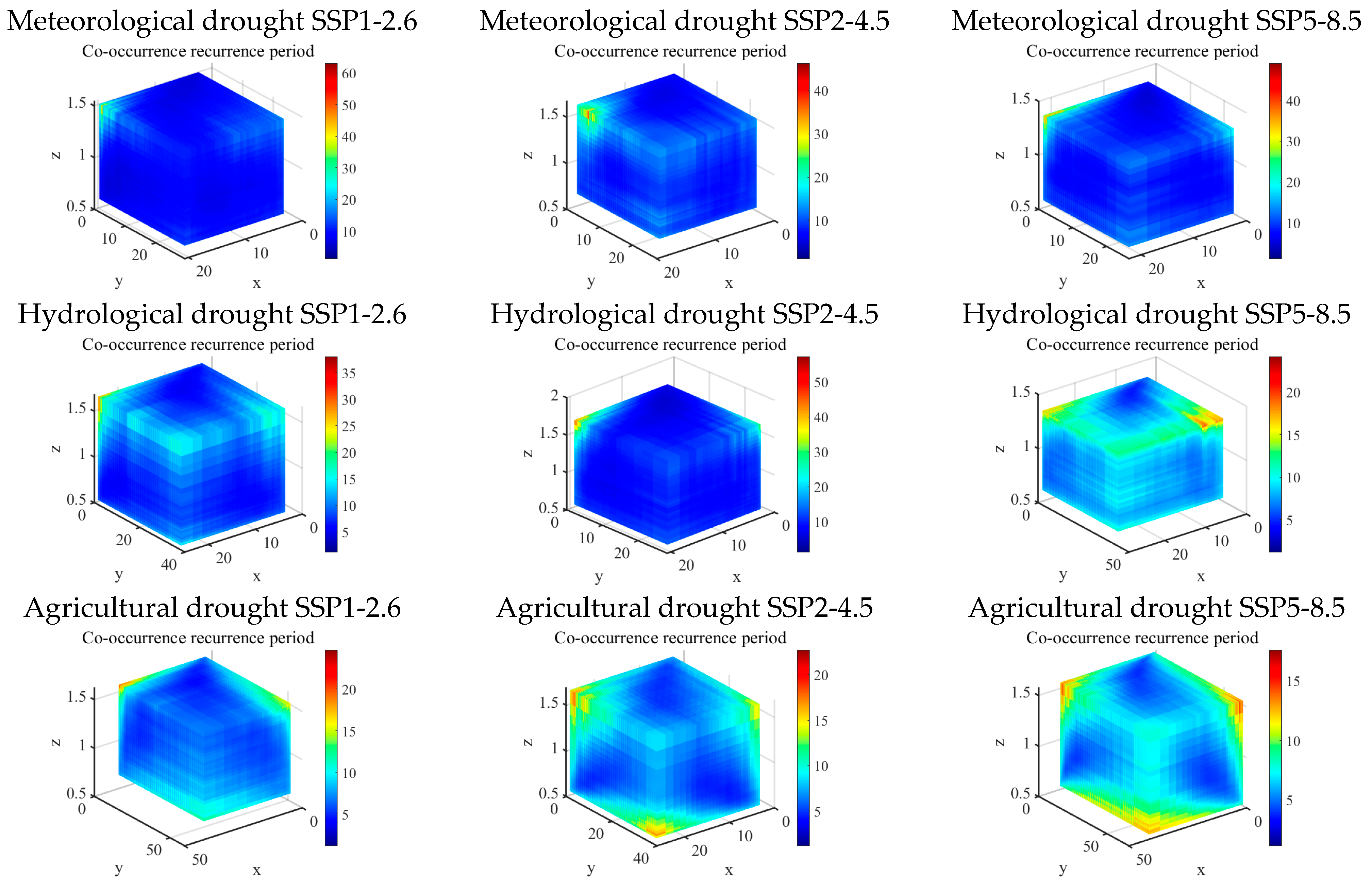
4.6.5. Three-Dimensional Reconstruction Period

Figure 10 and Figure 11 display the three-dimensional recurrence intervals of agricultural drought under “or” and “and” conditions across different scenarios, with data sourced from the frequency distribution of univariate drought characteristics. For meteorological drought, the return periods (R-o, R-a) at the 75%, 50%, and 25% thresholds are respectively: SSP1-2.6 (1.04, 1.39), (1.28, 2.77), (2.24, 6.28) years; SSP2-4.5: (1.07, 1.57), (1.43, 2.98), (1.93, 4.68) years; SSP5-8.5: (1.07, 1.53), (1.30, 2.39), (2.44, 6.60) years. For hydrological drought, the return periods are: SSP1-2.6 (1.07, 2.63), (1.32, 1.97), (2.12, 3.83) years; SSP2-4.5: (1.10, 1.69), (1.23, 2.48), (2.26, 7.17) years; SSP5-8.5: (1.06, 1.42), (1.27, 2.00), (2.33, 5.13) years. For agricultural drought, the return periods are: SSP1-2.6 (1.07, 1.46), (1.20, 1.98), (1.96, 3.62) years; SSP2-4.5: (1.09, 1.31), (1.33, 1.74), (1.81, 2.72) years; SSP5-8.5: (1.04, 1.25), (1.35, 1.56), (3.17, 4.44) years.

4.6.6. The Transmission Time from Meteorological Drought to Hydrological Drought and Agricultural Drought

This study selects SPAEI, SRI, and SSMI at 3, 6, and 12-month scales to calculate their lag correlations. Under the SSP1-2.6 scenario, the transmission times of meteorological drought to hydrological drought and agricultural drought at 3, 6, and 12-month scales are 8, 4, and 6 months, and 2, 4, and 5 months, respectively. Under the SSP2-4.5 scenario, the transmission times of meteorological drought to hydrological drought and agricultural drought at 3, 6, and 12-month scales are 8, 5, and 1 months, and 2, 4, and 4 months, respectively. Under the SSP5-8.5 scenario, the transmission times of meteorological drought to hydrological drought and agricultural drought at 3, 6, and 12-month scales are 7, 5, and 2 months, and 1, 3, and 5 months, respectively. These results reveal significant variability in drought propagation times across different emission scenarios and timescales, which is attributable to several interrelated mechanisms. Firstly, under high-emission scenarios (SSP5-8.5), a notable reduction in propagation time is evident, particularly at the monthly scale. Here, the transition from meteorological to hydrological drought decreases from six months (SSP1-2.6) to two months. This acceleration is primarily due to enhanced evapotranspiration, driven by rising temperatures, which intensifies soil moisture depletion and accelerates the circulation of surface water. Furthermore, increased precipitation variability and heightened intensity of extreme events under high-emission scenarios may exacerbate drought development rates while reducing the buffering capacity of hydrological systems. Secondly, distinct scale-dependent response characteristics were identified. At the monthly scale, propagation of meteorological drought to hydrological drought exhibited a longer lag time (7–8 months) across all scenarios. In contrast, the transition from meteorological to agricultural drought was more rapid (1–2 months). This pattern reflects the differing response mechanisms of soil moisture and runoff to precipitation deficits. The shallow root zone responds immediately to meteorological anomalies through direct precipitation–soil moisture interactions. In contrast, runoff generation requires the accumulation of runoff processes and groundwater recharge, resulting in longer lag times. Conversely, under the SSP5-8.5 scenario, the propagation of hydrological drought significantly accelerated at the 12-month scale (from 2 to 5 months), indicating that prolonged climate stress alters the relative response rates of different water storage components.

4.6.7. Transmission Risks from Meteorological Drought to Hydrological Drought and Agricultural Drought

Table 5 shows the probability of agricultural drought occurrence under different meteorological drought conditions. Under the SSP1-2.6 scenario, mild meteorological drought leads to an agricultural drought probability of 0.25 (mild) and 0.02 (extreme). Under the SSP2-4.5 scenario, the probability during mild meteorological drought is 0.28 (mild) and 0.03 (extreme), rising to 0.17 and 0.24 during extreme meteorological drought. Under SSP5-8.5, the probability during mild meteorological droughts is 0.26 and 0.03, increasing to 0.18 and 0.21 under extreme conditions. As meteorological drought severity increases, the probability of agricultural drought rises across all scenarios.
Table 6 shows the probability of hydrological drought occurrence under different meteorological drought conditions. Under the SSP1-2.6 scenario, the probability of hydrological drought resulting from mild meteorological drought is 0.18 (mild) and 0.03 (extreme), rising to 0.21 and 0.08 during extreme meteorological drought. Under the SSP2-4.5 scenario, probabilities shift from 0.16 and 0.06 (mild meteorological drought) to 0.12 and 0.34 (extreme meteorological drought), with a significant increase in extreme hydrological drought probability. The SSP5-8.5 scenario has the most severe impact: probabilities shift from 0.18 and 0.05 to 0.13 and 0.41, with the probability of extreme hydrological drought reaching the highest value across all scenarios (0.41).

4.6.8. Transmission Thresholds from Meteorological Drought to Hydrological Drought and Agricultural Drought

Under the SSP1-2.6 scenario, the occurrence threshold for mild agricultural drought is −1.9, while the probabilities for moderate, severe, and extreme agricultural droughts are all below the preset conditional probability, indicating that none of these three drought categories reached their thresholds. Under the SSP2-4.5 scenario, the occurrence thresholds for mild, moderate, severe, and extreme agricultural droughts are −1.1, −2.9, −3.4, and −3.9, respectively. Under the SSP5-8.5 scenario, the occurrence thresholds for mild, moderate, severe, and extreme agricultural droughts are −0.6, −1.2, −1.5, and −1.8, respectively.
Under the SSP1-2.6 scenario, the occurrence thresholds for mild, moderate, severe, and extreme hydrological droughts are −0.7, −1.7, −2.7, and −3.6, respectively. Under the SSP2-4.5 scenario, the occurrence threshold for mild hydrological drought is −0.6, while the probabilities for moderate, severe, and extreme hydrological droughts all fall below the preset conditional probability, indicating that none of these three drought types reach their thresholds. Under the SSP5-8.5 scenario, the occurrence thresholds for mild, moderate, severe, and extreme hydrological droughts are −0.6, −1.5, −2.8, and −4.5, respectively.

5. Discussion

This study systematically analyzed the joint probability and recurrence interval evolution of meteorological, hydrological, and agricultural drought characteristics in the lower reaches of the Songhua River basin under different SSP climate scenarios by constructing a two-dimensional and three-dimensional joint drought probability model. It further explored the propagation mechanisms of meteorological drought to hydrological and agricultural droughts and their associated risk thresholds [50].
The study indicates that the joint occurrence probability of droughts generally decreases significantly with increasing drought characteristic intensity, reflecting the difficulty of strong drought events simultaneously meeting the conditions of high values for multiple characteristic variables [51]. However, our results reveal a crucial distinction: the rate of probability decline varies significantly across different SSP scenarios—a phenomenon that has not been sufficiently explored in earlier studies primarily focused on historical periods [52]. Consistent with copula-based drought studies [53], strong dependency constraints in joint occurrences hold under both “OR” and “AND” logical conditions. However, our analysis goes further than previous studies by revealing scenario-specific variations in dependency structures. In the SSP5-8.5 scenario, disruption to traditional dependency patterns suggests that climate change could alter the co-evolutionary mechanisms of drought characteristics fundamentally, challenging the stationarity assumptions commonly used in earlier multivariate drought frameworks. This non-stationarity has significant implications for modelling drought risk, as conventional approaches based on historical dependency structures may underestimate the complexity of future droughts [54]. Significant changes in the combination patterns of D-S, D-P and S-P under moderate drought intensity (cumulative frequency of 50%) are a novel finding with important practical implications. Previous studies have primarily focused on extreme events, potentially overlooking the high sensitivity of moderate-intensity droughts to climate forcing. Our findings suggest that these more frequent, population-impacting events may be more reliable indicators of the impacts of climate change than rare extremes. This challenges the traditional emphasis on tail risks in the literature on drought [55] and calls for a shift in the design of early warning systems towards monitoring moderate-intensity compound events. The joint occurrence probability under OR logic consistently exceeds that under AND logic, consistent with fundamental probability principles. However, the scenario-dependent decline rate warrants further investigation. Under the SSP1-2.6 scenario, higher joint probabilities indicate sustained coherence in drought propagation chains, suggesting that mitigation pathways maintain the predictability of compound drought events. Conversely, under SSP5-8.5, despite increased marginal drought frequency [56], the joint probability of extreme intensity events is lowest, revealing a paradox: enhanced warming generates more frequent but less synchronized multidimensional droughts. This decoupling phenomenon, rarely documented in existing literature, may reflect competing processes—such as heightened evaporation demands and altered precipitation patterns—disrupting traditional drought propagation pathways [57].
From the perspective of drought propagation, we find that the conclusion “the lag of hydrological drought is generally longer than that of agricultural drought” aligns with the understanding that “the storage and regulation filter formed by the basin-reservoir-groundwater system delays and attenuates meteorological deficit signals” [58]. Multi-basin studies similarly indicate that the propagation time from meteorological drought (MD) to agricultural drought (AD) is typically shorter than that from MD to hydrological drought (HD), exhibiting differences across spatiotemporal scales dominated by soil water memory and aquifer response [59]. Under CMIP6 scenarios, propagation times for SSP1-2.6 and SSP5-8.5 are broadly comparable, consistent with prior findings that “propagation mechanisms remain relatively robust despite divergent precipitation forcings.” In contrast, the more pronounced propagation time differences observed under SSP2-4.5 align with reports indicating greater regional variability and higher uncertainties in meteorological drivers and land-atmosphere feedbacks under moderate forcing scenarios. Collectively, future research should enhance explicit characterization of surface-groundwater coupling and human-driven processes to improve the physical consistency of cross-scale propagation simulations.
The occurrence risk of agricultural drought (AD) and hydrological drought (HD) increases with the severity of meteorological drought (MD), but this increase exhibits a pronounced nonlinear pattern. Two key findings align with prior research: First, even mild MD can evolve into moderate to severe AD under conditions of soil water memory and enhanced land-atmosphere coupling. Studies based on conditional probability and thresholds indicate that in humid/karst or “greening” contexts, the trigger threshold for MD→AD transition is lower with a non-zero probability [60]. Second, HD exhibits heightened sensitivity to “substantial and persistent” meteorological anomalies (deep precipitation deficits coupled with elevated evapotranspiration demands): as MD intensifies, HD occurrence probability increases and propagation time shortens, though basin storage/discharge dynamics and engineering regulation modulate this sensitivity [61]. Collectively, these findings reinforce the necessity of explicitly modeling threshold behaviors and nonlinear feedback in cross-sectoral propagation simulations.
Our threshold analysis reveals a “trigger point” characteristic in drought propagation: once meteorological drought (MD) reaches a certain intensity, the occurrence probability of agricultural drought (AD) and hydrological drought (HD) exhibits a nonlinear jump. This aligns with the quantitative characterization of propagation thresholds based on the Copula-based conditional probability framework [62]. Simultaneously, we find that the propagation thresholds for AD are generally lower than those for HD. This aligns with literature findings indicating a more direct “MD-soil water” threshold-based feedback, while HD triggering is more heavily modulated by processes such as basin storage and discharge regulation, engineering controls, and baseflow dynamics. Scenario comparisons further support this insight: under SSP1-2.6, many moderate-to-severe MD events failed to cross established thresholds, exhibiting stronger buffering capacity. Conversely, under SSP5-8.5, multi-level droughts exhibited distinct and lower propagation thresholds, consistent with projections of increased propagation probability and heightened triggering of severe AD/HD under warming conditions. In summary, integrating existing research, we emphasize the need to explicitly model threshold behavior and human-nature interactions (evaporation, infiltration, storage/dispatch) to avoid underestimating the rapid transition from MD to AD/HD under high-emission scenarios [63].
Our results for binary-ternary recurrence intervals show that recurrence intervals under “AND” conditions are systematically longer than those under “OR” conditions, consistent with multivariate frequency theory—design events defined by intersection are rarer than those defined by union, leading to distinct recurrence interval contour patterns. The greatest AND–OR discrepancy was observed at approximately 25% cumulative frequency, indicating higher sensitivity of severe droughts to climate change [64]. This aligns with assessments suggesting warming disproportionately amplifies extreme events and with CMIP6-based ternary analyses detecting more pronounced changes at high intensity levels. Simultaneously, the markedly distinct contour patterns under “AND” and “OR” conditions validate a core finding in compound event research: when hazard factors/attributes are correlated, univariate methods underestimate co-occurrence risks, necessitating multivariate design and risk metrics to characterize drought [65].
This study demonstrates remarkable comprehensiveness and innovation in drought risk assessment methodology. Unlike most CMIP6-based drought studies in mainland China that rely on traditional SPI or SPEI indices [66], this research introduces the SPAEI index, which accounts for actual evapotranspiration. It further integrates SRI and SSMI to establish a three-dimensional meteorological–hydrological–agricultural drought monitoring system. This multi-index analysis framework addresses the limitations of previous Chinese drought studies, which primarily relied on single or two-dimensional drought indicators [67], enabling a more comprehensive characterization of the propagation mechanisms of different drought types. Regarding future scenario simulations, unlike most existing studies in Northeast China that employ the SWAT model combined with CMIP5 data or single land-use scenarios [68,69], this research innovatively integrates the latest CMIP6 climate scenarios with dynamic land-use changes projected by the PLUS model. Recent studies on the Liaohe River basin demonstrate that the PLUS model exhibits excellent adaptability in simulating Northeast China’s land use, achieving overall accuracy exceeding 0.93 and Kappa coefficients greater than 0.85. These results align with the high-precision validation obtained in this study (Kappa = 0.83, OA = 0.92), confirming the applicability of this methodological framework to the lower reaches of the Songhua River basin. Regarding multidimensional drought risk analysis methods, although Copula functions and Bayesian networks have been applied in regions such as the Yangtze River Basin, Yellow River Basin, and arid zones of Central Asia in China [70], integrated frameworks combining both with CMIP6 multi-model ensembles and machine learning algorithms remain relatively uncommon. This study quantifies the joint occurrence probability of different combinations of drought characteristic variables using Copula conditional probability. It further employs Bayesian networks to reveal propagation thresholds for meteorological, hydrological, and agricultural droughts. Methodologically, this approach transcends the limitations of previous studies in Southwest and Central China, which primarily focused on two-dimensional drought frequency analysis. Notably, the drought trigger threshold identification method based on Copula-Bayesian conditional probability theory [71], along with the application of complex network theory in studying drought propagation mechanisms [72], has demonstrated promising results in the Yangtze and Pearl River basins. This study introduces these advanced methods to the lower reaches of the Songhua River Basin, implementing adaptive modifications tailored to the characteristics of high-latitude semi-humid climatic zones. Unlike national-scale studies that employ three-dimensional clustering to identify drought event duration, severity, and affected area, this research precisely extracts characteristic variables such as drought duration, intensity, and peak values through run length theory, while quantifying non-stationary variations under different SSP scenarios. In summary, this study integrates multi-source data, multi-model coupling, and multidimensional statistical analysis methods to establish a comprehensive methodological framework spanning drought identification, propagation mechanisms, and risk assessment. This integrated framework not only surpasses previous regional studies in China that relied on single methodologies or two-dimensional analysis models in terms of technical approach, but also demonstrates high simulation accuracy and predictive capability when applied to the climate change-sensitive area of the lower Songhua River basin. It provides important methodological references for regional drought risk management under climate change.

6. Conclusions

1 Under different scenarios, the joint occurrence probability of droughts generally decreases as drought intensity increases, with a significant decline under both “OR” and “AND” logical conditions as drought characteristic variables increase. The largest decline is observed at moderate drought intensity (cumulative frequency of 50%), indicating that this intensity is the most sensitive to climate change.
2 Under the SSP1-2.6 and SSP5-8.5 scenarios, the joint occurrence probabilities of droughts are higher at medium to high cumulative frequencies (50% and 75%), while under the SSP5-8.5 scenario, the joint probability of extreme droughts is lower, suggesting that droughts are more extreme in high-emission scenarios but with reduced multidimensional linkage. The SSP2-4.5 scenario shows higher joint probabilities at low frequency (25%), reflecting a more complex drought pattern.
3 The transmission of meteorological drought to hydrological and agricultural droughts exhibits significant lag, with the lag increasing with temporal scale. Under the SSP1-2.6 scenario, the transmission time to hydrological drought is longer, indicating a slower feedback response in the hydrological system to meteorological drought. In contrast, the response time for agricultural drought is relatively shorter, reflecting the high sensitivity of the agricultural system to meteorological drought. As the level of meteorological drought increases, the occurrence probabilities of agricultural and hydrological droughts gradually rise, with extreme meteorological droughts having a particularly significant impact on both agricultural and hydrological systems.
4 Under the SSP5-8.5 scenario, the drought transmission thresholds are low, indicating faster drought propagation; under the SSP1-2.6 scenario, the thresholds are higher, suggesting a certain buffering effect.
5. Bivariate and trivariate return period analyses indicate that drought events consistently exhibit higher return periods under “AND” conditions than under “OR” conditions, with spatial contour patterns showing sparse and dense distributions, respectively. The most significant change occurred at the 25% cumulative frequency scenario, indicating that severe drought scenarios are most sensitive to future climate change. Furthermore, the recurrence intervals of meteorological, hydrological, and agricultural droughts exhibited high temporal consistency, reflecting the continuous propagation of drought signals through the atmosphere–land–agriculture system.
6. Mann–Kendall and Pettitt tests reveal markedly different temporal evolution patterns across SSP scenarios: SSP1-2.6 exhibits early improvements in SRI and SSMI (2030–2045), SSP2-4.5 exhibits a gradual transition, while SSP5-8.5 shows concentrated abrupt changes with the highest intensity (a 240% increase in SRI’s UT). Differentiated sensitivity of drought indices—SSMI responds most strongly, while SPEI is the most conservative.

Supplementary Materials

The following supporting information can be downloaded at https://www.mdpi.com/article/10.3390/hydrology12110287/s1. Figure S1: Land use Sankey diagram from 2000 to 2020. Figure S2: Contribution of Driving Factors to the Decrease in Arable and Forest Land Areas and the Increase in Built-up Land Area in the Lower Songhua River Basin. Figure S3: The areas of arable and forest land decrease and construction land expansion in the Lower Songhua River Basin were overlaid with their corresponding dominant contributing factors to identify the primary drivers of land use change. Figure S4: Predicted distribution of land use for typical SSPs-RCPs scenarios. Figure S5: Rate of change in land use area for typical SSPs-RCPs scenarios. Figure S6: Comparison of theoretical and empirical frequencies of multidimensional drought characteristic variables. Figure S7: Comparison of theoretical and empirical frequencies of multidimensional drought characteristic variables. Figure S8: Comparison of theoretical and empirical frequencies of multidimensional drought characteristic variables. Figure S9: Two-dimensional joint occurrence probability distribution of hydrological drought characteristic variables. Figure S10: Two-dimensional joint occurrence probability distribution of agricultural drought characteristic variables. Figure S11: Two-dimensional recurrence period of hydrological drought characteristic variables. Figure S12: Two-dimensional recurrence period of agricultural drought characteristic variables. Table S1: Driver information. Table S2: Land Use Transition Cost Matrix and Neighborhood Weights under Typical SSP–RCP Scenarios. Table S3: SWAT Model Parameterization for the Lower Songhua River Basin. Table S4: Drought Characteristics at Jiamusi Station Under Future Climate Scenarios. Table S5: AIC Test Results for Fitted Distributions of Drought Characteristic Variables under Different Periods and Types in the SSP1-2.6 Scenario. Table S6: AIC test results of fitted distributions for different types of drought characteristic variables across various time periods under the SSP2-4.5 scenario. Table S7: AIC test results of fitted distributions for different types of drought characteristic variables across various time periods under the SSP5-8.5 scenario. Table S8: The optimal Copula function under different combinations of meteorological drought characteristic variables across various time periods in the SSP1-2.6 scenario. Table S9: The optimal Copula function under different combinations of meteorological drought characteristic variables across various time periods in the SSP2-4.5scenario. Table S10: The optimal Copula function under different combinations of meteorological drought characteristic variables across various time periods in the SSP5-8.5 scenario. Table S11: The optimal Copula function under different combinations of hydrological drought characteristic variables across various time periods in the SSP1-2.6 scenario. Table S12: The optimal Copula function under different combinations of hydrological drought characteristic variables across various time periods in the SSP2-4.5 scenario. Table S13: The optimal Copula function under different combinations of hydrological drought characteristic variables across various time periods in the SSP5-8.5 scenario. Table S14: The optimal Copula function under different combinations of agricultural drought characteristic variables across various time periods in the SSP1-2.6 scenario. Table S15: The optimal Copula function under different combinations of agricultural drought characteristic variables across various time periods in the SSP2-4.5 scenario. Table S16: The optimal Copula function under different combinations of agricultural drought characteristic variables across various time periods in the SSP5-8.5scenario.

Author Contributions

Y.Z.: Conceptualization, Methodology, Formal analysis, Software, Data curation, Writing—original draft; Y.S. and C.D.: Supervision, Conceptualization, Writing—review & editing, Project administration; T.L.: Investigation, Data curation; X.H. and Z.W.: Investigation, Data curation. All authors have read and agreed to the published version of the manuscript.

Funding

This research received no external funding.

Data Availability Statement

The datasets used and/or analyzed during the current study are available from the corresponding author on reasonable request. The code and data processing in this study were conducted using MATLAB R2022a and Python (3.9).

Conflicts of Interest

The authors declare no conflict of interest.

References

  1. Ullah, I.; Mukherjee, S.; Syed, S.; Mishra, A.K.; Ayugi, B.O.; Aadhar, S. Anthropogenic and atmospheric variability intensifies flash drought episodes in South Asia. Commun. Earth Environ. 2024, 5, 267. [Google Scholar] [CrossRef]
  2. Berg, A.; Sheffield, J. Climate Change and Drought: The Soil Moisture Perspective. Curr. Clim. Change Rep. 2018, 4, 180–191. [Google Scholar] [CrossRef]
  3. Huang, Y.; Shen, L.; Liu, H. Grey relational analysis, principal component analysis and forecasting of carbon emissions based on long short-term memory in China. J. Clean. Prod. 2019, 209, 415–423. [Google Scholar] [CrossRef]
  4. Wang, H.; Wang, Z.; Bai, Y.; Wang, W. Propagation characteristics of meteorological drought to hydrological drought considering nonlinear correlations—A case study of the Hanjiang River Basin, China. Ecol. Inform. 2024, 80, 102512. [Google Scholar] [CrossRef]
  5. Wen, Y.; Liwei, Z.; Ling, K.; Hao, C.; Guo, J. Drought risk analysis based on multivariate copula function in Henan Province, China. Geomat. Nat. Hazards Risk 2023, 14, 2223344. [Google Scholar] [CrossRef]
  6. Zhao, Q.; Zhang, X.; Li, C.; Xu, Y.; Fei, J. Compound ecological drought assessment of China using a Copula-based drought index. Ecol. Indic. 2024, 164, 112141. [Google Scholar] [CrossRef]
  7. Jiang, C.; Ma, C.; Duan, S.; Min, X.; Zhang, Y.; Li, D.; Zhang, X. Monitoring of agricultural drought based on multi-source remote sensing data in Heilongjiang Province, China. J. Integr. Agric. 2025, in press. [Google Scholar] [CrossRef]
  8. Zhao, Q.; Zou, C.H.; Wang, K.F.; Gao, Q.; Yao, T. Spatial and Temporal Distribution Characteristics of Drought and Its Influencing Factors in Heilongjiang Province, China from 1956 to 2015. Appl. Ecol. Environ. Res. 2019, 17, 2631–2650. [Google Scholar] [CrossRef]
  9. Hua, Y.; Ye, L.; Zhang, H.; Zuo, H.; Zhou, H. Research on Multi-Variable Hydrological Drought Characteristics of the Lower Nenjiang River Basin. J. China Hydrol. 2021, 41, 88–94. [Google Scholar] [CrossRef]
  10. Liu, T.; Si, Z.; Zhao, Y.; Wang, J.; Liu, Y.; Wang, L. Drought Propagation and Risk Assessment in the Naoli River Basin Based on the SWAT-PLUS Model and Copula Functions. Sustainability 2025, 17, 8219. [Google Scholar] [CrossRef]
  11. Ding, Y.; Gong, X.; Xing, Z.; Cai, H.; Zhou, Z.; Zhang, D.; Sun, P.; Shi, H. Attribution of meteorological, hydrological and agricultural drought propagation in different climatic regions of China. Agric. Water Manag. 2021, 255, 106996. [Google Scholar] [CrossRef]
  12. Xie, Y.; Kang, C.; Chi, Y.; Wu, P.; Wei, Z.; Wang, J.; Sun, L. Reversal of the middle-upper Songhua River in the late Early Pleistocene, Northeast China. Geomorphology 2020, 369, 107373. [Google Scholar] [CrossRef]
  13. Yang, X.; Dai, C.; Liu, G.; Meng, X.; Li, C. Evaluation of Groundwater Resources in the Middle and Lower Reaches of Songhua River Based on SWAT Model. Water 2024, 16, 2839. [Google Scholar] [CrossRef]
  14. Arnold, J.G.; Srinivasan, R.; Muttiah, R.S.; Williams, J.R. Large area hydrologic modeling and assessment part I: Model development. JAWRA J. Am. Water Resour. Assoc. 1998, 34, 73–89. [Google Scholar] [CrossRef]
  15. Neitsch, S.L.; Arnold, J.G.; Kiniry, J.R.; Williams, J.R. Soil and Water Assessment Tool Theoretical Documentation; USDA–153 ARS Grassland Soil and Water Research Laboratory, and Texas A&M University; Blackland Research and Extension Center: Temple, TX, USA, 2011. [Google Scholar]
  16. Neitsch, S.L.; Arnold, J.G.; Kiniry, J.R.; Srinivasan, R.; Williams, J.R. Soil and Water Assessment Tool Input/Output File Documentation; USDA-ARS: USDA-ARS Grassland; Soil and Water Research Laboratory: Temple, TX, USA, 2012. [Google Scholar]
  17. Long, S.B.; Gao, J.E.; Shao, H.; Wang, L.; Zhang, X.C.; Gao, Z. Developing SWAT-S to strengthen the soil erosion forecasting performance of the SWAT model. Land Degrad. Dev. 2024, 35, 280–295. [Google Scholar] [CrossRef]
  18. Bayat, M.; Alizadeh, H.; Mojaradi, B. SWAT_DA: Sequential Multivariate Data Assimilation-Oriented Modification of SWAT. Water Resour. Res. 2022, 58, e2022WR032397. [Google Scholar] [CrossRef]
  19. Tan, M.L.; Gassman, P.W.; Srinivasan, R.; Arnold, J.G.; Yang, X. A Review of SWAT Studies in Southeast Asia: Applications, Challenges and Future Directions. Water 2019, 11, 914. [Google Scholar] [CrossRef]
  20. Jiang, A.; Zhang, W.; Liu, X.; Zhou, F.; Li, A.; Peng, H.; Wang, H. Improving hydrological process simulation in mountain watersheds: Integrating WRF model gridded precipitation data into the SWAT model. J. Hydrol. 2024, 639, 131687. [Google Scholar] [CrossRef]
  21. Xiang, K.Y.; Li, Y.; Horton, R.; Feng, H. Similarity and difference of potential evapotranspiration and reference crop evapotranspiration—A review. Agric. Water Manag. 2020, 232, 106043. [Google Scholar] [CrossRef]
  22. Abbaspour, K.C. SWAT-CUP: SWAT Calibration and Uncertainty Programs—A User Manual; Eawag: Dübendorf, Switzerland, 2015; p. 100. [Google Scholar]
  23. Zare, M.; Azam, S.; Sauchyn, D. Evaluation of Soil Water Content Using SWAT for Southern Saskatchewan, Canada. Water 2022, 14, 249. [Google Scholar] [CrossRef]
  24. Sánchez-Gómez, A.; Martínez-Pérez, S.; Pérez-Chavero, F.M.; Molina-Navarro, E. Optimization of a SWAT model by incorporating geological information through calibration strategies. Optim. Eng. 2022, 23, 2203–2233. [Google Scholar] [CrossRef]
  25. Ostad-Ali-Askari, K. Investigation of meteorological variables on runoff archetypal using SWAT: Basic concepts and fundamentals. Appl. Water Sci. 2022, 12, 177. [Google Scholar] [CrossRef]
  26. Moriasi, D.N.; Arnold, J.G.; van Liew, M.W.; Bingner, R.L.; Harmel, R.D.; Veith, T.L. Model Evaluation Guidelines for Systematic Quantification of Accuracy in Watershed Simulations. Trans. ASABE 2007, 50, 885–900. [Google Scholar] [CrossRef]
  27. Liu, J.; Kong, X.; Zhu, Y.; Zhang, B. A study on land use change simulation based on PLUS model and the U-net structure: A case study of Jilin Province. Ecol. Indic. 2025, 176, 113619. [Google Scholar] [CrossRef]
  28. Liu, J.; Liu, B.; Wu, L.; Miao, H.; Liu, J.; Jiang, K.; Ding, H.; Gao, W.; Liu, T. Prediction of land use for the next 30 years using the PLUS model’s multi-scenario simulation in Guizhou Province, China. Sci. Rep. 2024, 14, 13143. [Google Scholar] [CrossRef]
  29. Liang, X.; Guan, Q.; Clarke, K.C.; Liu, S.; Wang, B.; Yao, Y. Understanding the drivers of sustainable land expansion using a patch-generating land use simulation (PLUS) model: A case study in Wuhan, China. Comput. Environ. Urban Syst. 2021, 85, 101569. [Google Scholar] [CrossRef]
  30. Zhang, Y.; Du, S.; Zhu, L.; Guo, T.; Zhao, X.; Guo, J. Sub-District Level Spatiotemporal Changes of Carbon Storage and Driving Factor Analysis: A Case Study in Beijing. Land 2025, 14, 151. [Google Scholar] [CrossRef]
  31. Jafari, T.; Kiem, A.S.; Javadi, S.; Nakamura, T.; Nishida, K. Fully integrated numerical simulation of surface water-groundwater interactions using SWAT-MODFLOW with an improved calibration tool. J. Hydrol.-Reg. Stud. 2021, 35, 100822. [Google Scholar] [CrossRef]
  32. Abbas, S.A.; Xuan, Y.Q.; Bailey, R.T. Assessing Climate Change Impact on Water Resources in Water Demand Scenarios Using SWAT-MODFLOW-WEAP. Hydrology 2022, 9, 164. [Google Scholar] [CrossRef]
  33. Nie, Y.F.; Lin, X.; Yang, Q.H.; Liu, J.P.; Chen, D.; Uotila, P. Differences Between the CMIP5 and CMIP6 Antarctic Sea Ice Concentration Budgets. Geophys. Res. Lett. 2023, 50, e2023GL105265. [Google Scholar] [CrossRef]
  34. Lu, Y.; Yang, T.; Fu, J.; Song, W. Utility of the standardized precipitation evapotranspiration index (SPEI) to detect agricultural droughts over China. J. Hydrol. Reg. Stud. 2025, 58, 102190. [Google Scholar] [CrossRef]
  35. GB/T 20481—2017; Grades of Meteorological Drought. Standards Press of China: Beijing, China, 2017.
  36. McCabe, S. Theory in tourism. Ann. Tour. Res. 2024, 104, 103721. [Google Scholar] [CrossRef]
  37. Pan, Y.; Zhu, Y.; Lü, H.; Yagci, A.L.; Fu, X.; Liu, E.; Xu, H.; Ding, Z.; Liu, R. Accuracy of agricultural drought indices and analysis of agricultural drought characteristics in China between 2000 and 2019. Agric. Water Manag. 2023, 283, 108305. [Google Scholar] [CrossRef]
  38. Wang, Y.; Zhang, X.; Zhou, N.; Hu, Z.; Li, J.; Lv, Y.; Wang, Y. Evolution characteristics of global meteorological and hydrologicaldisasters from 1990 to 2019. Trans. Atmos. Sci. 2021, 44, 496–506. [Google Scholar] [CrossRef]
  39. Shen, C. Analysis of detrended time-lagged cross-correlation between two nonstationary time series. Phys. Lett. A 2015, 379, 680–687. [Google Scholar] [CrossRef]
  40. Wu, J.; Chen, X.; Yao, H.; Gao, L.; Chen, Y.; Liu, M. Non-linear relationship of hydrological drought responding to meteorological drought and impact of a large reservoir. J. Hydrol. 2017, 551, 495–507. [Google Scholar] [CrossRef]
  41. Sklar, A. Fonctions de Repartition a n Dimensions et Leurs Marges; Université Paris 8: Saint-Denis, France, 1959. [Google Scholar]
  42. Rüschendorf, L. Transform. In Mathematical Risk Analysis: Dependence, Risk Bounds, Optimal Allocations and Portfolios; Rüschendorf, L., Ed.; Springer: Berlin/Heidelberg, Germany, 2013; pp. 3–34. [Google Scholar]
  43. Li, Z.L.; Shao, Q.X.; Tian, Q.Y.; Zhang, L.I. Copula-based drought severity-area-frequency curve and its uncertainty, a case study of Heihe River basin, China. Hydrol. Res. 2020, 51, 867–881. [Google Scholar] [CrossRef]
  44. Esit, M.; Yuce, M.I. Copula-based bivariate drought severity and duration frequency analysis considering spatial-temporal variability in the Ceyhan Basin, Turkey. Theor. Appl. Climatol. 2023, 151, 1113–1131. [Google Scholar] [CrossRef]
  45. Chattopadhyay, S. Finite mixture copulas for modeling dependence in longitudinal count data. METRON 2025, 83, 183–212. [Google Scholar] [CrossRef]
  46. Rohmer, J. Uncertainties in conditional probability tables of discrete Bayesian Belief Networks: A comprehensive review. Eng. Appl. Artif. Intell. 2020, 88, 103384. [Google Scholar] [CrossRef]
  47. Maina, S.C.; Mwigereri, D.; Weyn, J.; Mackey, L.; Ochieng, M. Evaluation of Dependency Structure for Multivariate Weather Predictors Using Copulas. ACM J. Comput. Sustain. Soc. 2023, 1, 17. [Google Scholar] [CrossRef]
  48. Zhou, S.; Qu, Y.; Wang, Y.; Wu, Z.; Shi, Y. Ecosystem service bundles under SSP-RCP and local scenarios: A pathway to comprehensive spatial planning for sustainability. Resour. Environ. Sustain. 2025, 20, 100211. [Google Scholar] [CrossRef]
  49. Wang, F.; Wang, Z.; Yang, H.; Di, D.; Zhao, Y.; Liang, Q.; Hussain, Z. Comprehensive evaluation of hydrological drought and its relationships with meteorological drought in the Yellow River basin, China. J. Hydrol. 2020, 584, 124751. [Google Scholar] [CrossRef]
  50. Sun, P.; Liu, R.; Yao, R.; Gu, X.; Gulakhmadov, A.; Kong, D.; Zhang, X. Propagation threshold from meteorological to agricultural drought and its potential influence factors. J. Hydrol. 2025, 655, 132920. [Google Scholar] [CrossRef]
  51. Zhao, R.; Wang, H.; Hu, S.; Zhan, C.; Guo, J. Joint probability of drought encounter among three major grain production zones of China under nonstationary climate. J. Hydrol. 2021, 603, 126995. [Google Scholar] [CrossRef]
  52. Mesbahzadeh, T.; Mirakbari, M.; Mohseni Saravi, M.; Soleimani Sardoo, F.; Miglietta, M.M. Meteorological drought analysis using copula theory and drought indicators under climate change scenarios (RCP). Meteorol. Appl. 2020, 27, e1856. [Google Scholar] [CrossRef]
  53. Kao, S.-C.; Govindaraju, R.S. A copula-based joint deficit index for droughts. J. Hydrol. 2010, 380, 121–134. [Google Scholar] [CrossRef]
  54. Yang, X.; Li, Y.P.; Huang, G.H.; Li, Y.F.; Liu, Y.R.; Zhou, X. Development of a multi-GCMs Bayesian copula method for assessing multivariate drought risk under climate change: A case study of the Aral Sea basin. CATENA 2022, 212, 106048. [Google Scholar] [CrossRef]
  55. Mirabbasi, R.; Fakheri-Fard, A.; Dinpashoh, Y. Bivariate drought frequency analysis using the copula method. Theor. Appl. Climatol. 2012, 108, 191–206. [Google Scholar] [CrossRef]
  56. Cook, B.I.; Mankin, J.S.; Marvel, K.; Williams, A.P.; Smerdon, J.E.; Anchukaitis, K.J. Twenty-First Century Drought Projections in the CMIP6 Forcing Scenarios. Earth’s Future 2020, 8, e2019EF001461. [Google Scholar] [CrossRef]
  57. Liu, H.; Guo, C.; Jiang, S.; Zhang, K. Effect of water distribution on methane-carbon dioxide-water transportation in shale nanopores with Knudsen number correction. J. Hydrol. 2024, 645, 132186. [Google Scholar] [CrossRef]
  58. Van Loon, A.F. Hydrological drought explained. WIREs Water 2015, 2, 359–392. [Google Scholar] [CrossRef]
  59. Zhou, Z.; Shi, H.; Fu, Q.; Ding, Y.; Li, T.; Liu, S. Investigating the Propagation From Meteorological to Hydrological Drought by Introducing the Nonlinear Dependence With Directed Information Transfer Index. Water Resour. Res. 2021, 57, e2021WR030028. [Google Scholar] [CrossRef]
  60. Xu, Z.; Wu, Z.; Shao, Q.; He, H.; Guo, X. From meteorological to agricultural drought: Propagation time and probabilistic linkages. J. Hydrol. Reg. Stud. 2023, 46, 101329. [Google Scholar] [CrossRef]
  61. Du, M.; Liu, Y.; Huang, S.; Zheng, H.; Huang, Q. Probability-Based Propagation Characteristics from Meteorological to Hydrological Drought and Their Dynamics in the Wei River Basin, China. Water 2024, 16, 1999. [Google Scholar] [CrossRef]
  62. Liu, Q.; Yang, Y.; Liang, L.; Jun, H.; Yan, D.; Wang, X.; Li, C.; Sun, T. Thresholds for triggering the propagation of meteorological drought to hydrological drought in water-limited regions of China. Sci. Total Environ. 2023, 876, 162771. [Google Scholar] [CrossRef] [PubMed]
  63. Wang, H.; Zhu, Y.; Qin, T.; Zhang, X. Study on the propagation probability characteristics and prediction model of meteorological drought to hydrological drought in basin based on copula function. Front. Earth Sci. 2022, 10, 961871. [Google Scholar] [CrossRef]
  64. Salvadori, G.; De Michele, C.; Durante, F. On the return period and design in a multivariate framework. Hydrol. Earth Syst. Sci. 2011, 15, 3293–3305. [Google Scholar] [CrossRef]
  65. Zscheischler, J.; Seneviratne, S.I. Dependence of drivers affects risks associated with compound events. Sci. Adv. 2017, 3, e1700263. [Google Scholar] [CrossRef]
  66. Xu, Y.; Zhang, X.; Hao, Z.; Hao, F.; Li, C. Projections of future meteorological droughts in China under CMIP6 from a three-dimensional perspective. Agric. Water Manag. 2021, 252, 106849. [Google Scholar] [CrossRef]
  67. Ayantobo, O.O.; Li, Y.; Song, S. Multivariate Drought Frequency Analysis using Four-Variate Symmetric and Asymmetric Archimedean Copula Functions. Water Resour. Manag. 2019, 33, 103–127. [Google Scholar] [CrossRef]
  68. Liu, T.; Si, Z.; Liu, Y.; Wang, L.; Zhao, Y.; Wang, J. Runoff and Drought Responses to Land Use Change and CMIP6 Climate Projections. Water 2025, 17, 1696. [Google Scholar] [CrossRef]
  69. Liu, H.; Liu, J.; Chen, W. Effects of climate and land use change on runoff of the Second Songhua River Basin guided by SWAT model. Water Supply 2024, 24, 707–722. [Google Scholar] [CrossRef]
  70. Wang, T.; Tu, X.; Singh, V.P.; Chen, X.; Lin, K.; Zhou, Z.; Zhu, J. A CMIP6-based framework for propagation from meteorological and hydrological droughts to socioeconomic drought. J. Hydrol. 2023, 623, 129782. [Google Scholar] [CrossRef]
  71. Li, P.; Huang, Q.; Huang, S.; Leng, G.; Peng, J.; Wang, H.; Zheng, X.; Li, Y.; Fang, W. Various maize yield losses and their dynamics triggered by drought thresholds based on Copula-Bayesian conditional probabilities. Agric. Water Manag. 2022, 261, 107391. [Google Scholar] [CrossRef]
  72. Gao, C.; Liu, L.; Zhang, S.; Xu, Y.-P.; Wang, X.; Tang, X. Spatiotemporal patterns and propagation mechanism of meteorological droughts over Yangtze River Basin and Pearl River Basin based on complex network theory. Atmos. Res. 2023, 292, 106874. [Google Scholar] [CrossRef]
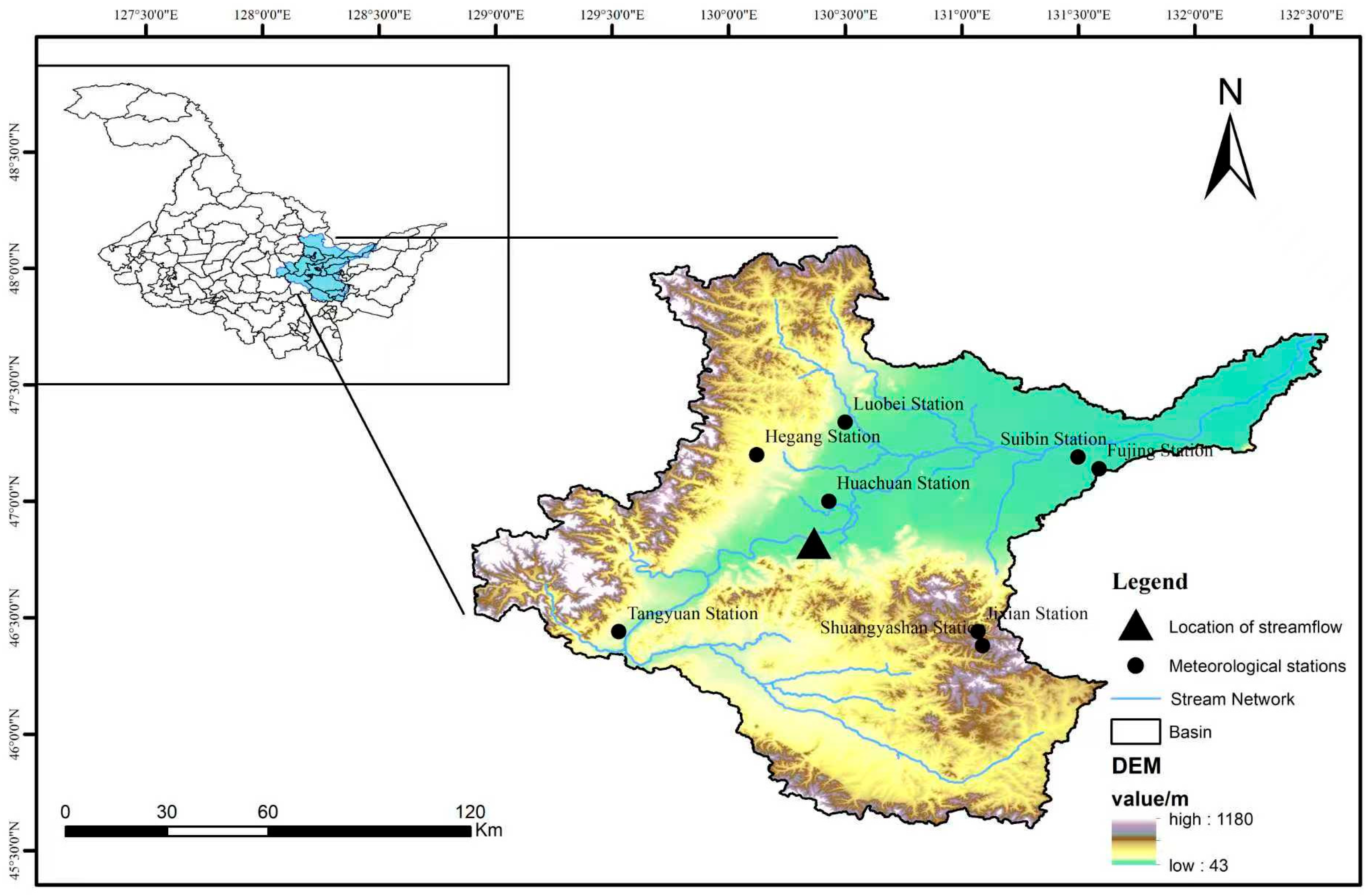
Figure 1. Distribution of water systems and hydrological stations in the lower Songhua River Basin.
Hydrology 12 00287 g001
Figure 2. Research Methodology Framework Diagram.
Hydrology 12 00287 g002
Figure 3. Relative Performance of Different GCMs in Simulating Maximum Temperature, Minimum Temperature, and Precipitation Compared with Observations (1970–2014). (a) Taylor Diagram for Watershed Rainfall. (b) Taylor diagram of the basin’s maximum temperature. (c) Taylor diagram of the basin’s minimum temperature.
Hydrology 12 00287 g003
Figure 4. Monthly runoff simulation results of Jiamusi hydrological station.
Hydrology 12 00287 g004
Figure 5. Trends and Discontinuities in Drought Indices Across Different Scenarios. (ac) show the M-K trend plots for meteorological, hydrological, and agricultural drought indices under three scenarios, respectively. (df) show the p-value plots for the meteorological, hydrological, and agricultural drought indices under three scenarios, respectively.
Hydrology 12 00287 g005
Figure 6. Two-dimensional joint occurrence probability distribution of meteorological drought characteristic variables.
Hydrology 12 00287 g006aHydrology 12 00287 g006b
Figure 7. Joint occurrence probability of three-dimensional drought under the ‘OR’ condition.
Hydrology 12 00287 g007
Figure 8. Joint occurrence probability of three-dimensional drought under the ‘AND’ condition.
Hydrology 12 00287 g008
Figure 9. Two-dimensional recurrence period of meteorological drought characteristic variables.
Hydrology 12 00287 g009aHydrology 12 00287 g009b
Figure 10. Three-dimensional drought recurrence period under “OR” conditions.
Hydrology 12 00287 g010
Figure 11. Three-dimensional drought recurrence period under “AND” conditions.
Hydrology 12 00287 g011
Table 1. Basic Information of Data Sources.
Data TypeResolutionSourceUse
Meteorological data China Meteorological Data NetworkConFigureuring the SWAT weather generator
CMIP62.8° × 2.8°Nasa Center for Climate SimulationPredicting future climate change
DEM90 mGeospatial Data CloudGeneration of river networks, delineation of sub-basins
Soil type1 kmHWSD Soil DatabaseBuilding a Soil Database
Land use1 kmCAS Data CentreClassification of land use types
Hydrological data Jiamusi Station Hydrological YearbookStreamflow simulation, rate determination and validation
Table 2. Basic Information of CMIP6 Climate Models.
Model NameResolution After Downscaling (°)Atmospheric Mode Resolution (°)Nations
MIROC-ES2L0.25 × 0.252.8 × 2.8Japan
ACCESS-ESM1-50.25 × 0.251.25 × 1.25Australia
NorESM2-LM0.25 × 0.251.9 × 2.5Norway
INM-CM4-80.25 × 0.251.5 × 1.5Russian
ACCESS-CM20.25 × 0.251.25 × 1.25Australia
CanESM50.25 × 0.252.8 × 2.8Canadian
EC-Earth30.25 × 0.250.25 × 0.25European multinational
GFDL-ESM40.25 × 0.251 × 1USA
INM-CM4-80.25 × 0.251.5 × 1.5Russian
IPSL-CM6A-LR0.25 × 0.251.875 × 1.875French
MIROC60.25 × 0.251.4 × 1.4Japan
MPI-ESM1-2-LR0.25 × 0.251.875 × 1.875German
MRI-ESM2-00.25 × 0.251.125 × 1.125Japan
Table 3. Hydrological Drought Classification Criteria.
LevelTypeSSP1-2.6, SSP2-4.5, SSP5-8.5
1No droughtSRI > −0.5
2Light drought−0.5 ≥ SRI > −1.0
3Moderate drought−1.0 ≥ SRI > −1.5
4Severe drought−1.5 ≥ SRI > −2.0
5Extreme droughtSRI ≤ −2.0
Note: The scenario names SSP1-2.6, SSP2-4.5, and SSP5-8.5 in the table are not drought classification criteria.
Table 4. Drought characteristic variables corresponding to different accumulation frequencies.
SituationMeteorological Drought
D ¯ /Month S ¯ P ¯
75%50%25%75%50%25%75%50%25%
SSP1-2.63.009.0014.002.379.1520.960.720.831.26
SSP2-4.54.0011.0012.004.0510.7916.700.840.991.30
SSP5-8.53.007.0012.002.345.0616.320.780.871.17
Hydrological drought
SSP1-2.63.0010.0016.002.527.1119.250.650.781.11
SSP2-4.54.006.0012.004.267.7915.630.810.921.46
SSP5-8.56.009.0016.003.967.0123.110.660.951.13
Agricultural drought
SSP1-2.610.0013.0019.006.5213.9425.410.740.911.49
SSP2-4.56.0012.0014.003.819.9823.500.660.811.11
SSP5-8.54.5012.0031.002.5010.2942.200.550.821.35
Table 5. Conditional Probabilities of Agricultural Drought under Different Meteorological Drought Scenarios.
SituationMeteorological Drought GradeAgricultural Drought Grade: 2Agricultural Drought Grad: 3Agricultural Drought Grad: 4Agricultural Drought Grad: 5
SSP1-2.620.180.100.050.03
30.200.120.060.04
40.210.130.070.06
50.210.150.080.08
SSP2-4.520.160.100.050.06
30.170.120.080.10
40.100.130.170.18
50.120.120.110.34
SSP5-8.520.180.110.060.05
30.190.150.090.11
40.180.160.130.21
50.130.140.140.41
Note: Drought grades 2, 3, 4, and 5, respectively, represent mild, moderate, severe, and extreme droughts.
Table 6. Conditional Probabilities of Hydrological Drought under Different Meteorological Drought Scenarios.
SituationMeteorological Drought GradeAgricultural Drought Grade: 2Agricultural Drought Grad: 3Agricultural Drought Grad: 4Agricultural Drought Grad: 5
SSP1-2.620.250.110.040.02
30.300.180.070.04
40.280.230.130.09
50.220.230.180.20
SSP2-4.520.280.170.070.03
30.270.240.130.06
40.230.260.190.12
50.170.240.230.24
SSP5-8.520.260.170.080.03
30.260.220.120.06
40.230.240.170.12
50.180.230.210.21
Note: Drought grades 2, 3, 4, and 5, respectively, represent mild, moderate, severe, and extreme droughts.
Disclaimer/Publisher’s Note: The statements, opinions and data contained in all publications are solely those of the individual author(s) and contributor(s) and not of MDPI and/or the editor(s). MDPI and/or the editor(s) disclaim responsibility for any injury to people or property resulting from any ideas, methods, instructions or products referred to in the content.