Article

Development of an Agricultural Water Risk Indicator Framework Using National Water Model Streamflow Forecasts

by
Joseph E. Quansah
1,*,
Ruben G. Doria
1,2,
Eniola E. Olakanmi
1 and
Souleymane Fall
1
1
Department of Agricultural and Environmental Sciences, Tuskegee University, Tuskegee, AL 36088, USA
2
EE SSW Water and Technology, WSP USA Inc., Birmingham, AL 35242, USA
*
Author to whom correspondence should be addressed.
Hydrology 2026, 13(2), 43; https://doi.org/10.3390/hydrology13020043 (registering DOI)
Submission received: 11 December 2025 / Revised: 17 January 2026 / Accepted: 21 January 2026 / Published: 24 January 2026

Abstract

Agricultural production remains highly susceptible to water-related risks, such as drought and flooding. Although hydrologic forecasting systems, such as the National Water Model (NWM), have advanced considerably, their outputs are rarely used for real-time agricultural decision-making. This study developed the Agricultural Water Risk Indicator (AWRI), a framework that translates NWM streamflow forecasts into crop-specific risk assessment indicators. The AWRI framework has three key components: (1) the hydrological threat and exposure characterization based on NWM streamflow forecasts (B1); (2) crop sensitivity by growth stage and water needs (B2); and (3) adaptive capacity reflecting the presence of irrigation or drainage infrastructure (B3). The AWRI was evaluated across three NWM reach IDs covering five farm sites in the Black Belt region of Alabama, USA. The results show that the AWRI captured variations in hydrologic conditions, risk, and crop tolerance across the research sites within the one- to four-week forecast range. Crops in the reproductive stage were especially sensitive. Without resilience measures, up to 55% of the crops simulated at some sites had high-risk AWRI categories. Including irrigation or drainage decreased risk scores by one to two levels. The AWRI tool provides farmers and stakeholders with critical information to support proactive agricultural water management.

1. Introduction

U.S. agriculture faces increasing hydrological threats from drought and flooding. These threats significantly impact crop yield, farm vulnerability, and water resource planning. Recent findings have shown that rain-fed crop systems, such as those used for growing corn, sorghum, soybeans, and spring wheat, are highly sensitive to hydroclimatic extremes, which results in yield losses [1]. These losses are not only spatially heterogeneous but are also strongly linked to crop insurance claims, indicating the need for tailored adaptive strategies for agricultural systems under water-related risks.
Flood events further complicate the agricultural landscape by disrupting soil structure, intensifying soil erosion, altering critical nutrient cycles, and reducing short- and long-term crop productivity [2]. While adaptation measures such as flood-tolerant crop varieties, improved drainage systems, and targeted soil amendments have been recommended, operational tools that support standardized risk assessment remain limited. The economic impact of floods and droughts on agriculture is substantial and persistent. Over the past few decades, U.S. agriculture has incurred average annual losses of approximately USD 3.99 billion due to flooding and USD 1.68 billion due to drought [3]. Although the overall trend in annual damage has remained relatively stable, this does not reflect the level of resilience or the impacts on different crops in different regions within the U.S. For instance, dryland systems generally experience more severe yield reductions during prolonged droughts than irrigated fields [4,5]. Some crops, and especially sensitive ones like corn, wheat, and soybeans, respond differently to water stress.
Social vulnerability exacerbates these hydrologic challenges. Across the U.S., agricultural communities exhibit varying degrees of exposure, sensitivity, and adaptive capacity. When hazard data are paired with socioeconomic indicators, disparities in hydrologic resilience become more apparent [6]. This complexity underscores the need for risk management frameworks. These frameworks must account not only for environmental stressors, but also for the varying abilities of communities to respond to them. Despite decades of research, most decision support tools exist as single or fragmented systems, with limited scalability and spatial relevance for proactive, farm-level planning. A study by [7] identified 81 tools related to agricultural water productivity; however, more than half of these tools are not publicly accessible.
To address this issue, researchers have been working to integrate climate indicators, crop sensitivity profiles, and adaptive capacity into composite risk assessments [8,9]. The growing intensity of weather extremes, especially long droughts and flash floods, demands an urgent need for operational tools that go beyond monitoring but instead provide forward-looking, actionable forecast-based systems [10,11,12]. Current efforts have largely focused on flood or drought impacts separately. For instance, a scoring matrix was developed by [13] to assess flood exposure across farm landscapes, while [14] grouped drought mitigation practices by their utility and farmer preferences. Spatial analyses of precipitation-yield relationships have also been used to explore streamflow uncertainty in flood-prone zones [10,15]. In some contexts, community-driven assessments and qualitative indicators have been applied to manage uncertainty in agricultural risk tracking [16,17]. Many of these studies have a common theme: the use of exposure, sensitivity, and adaptive capacity as foundational pillars of agricultural risk assessment [18,19]. However, few tools fully integrate all of these dimensions using real-time, validated hydrologic inputs.
Crop physiology is one of the most critical factors for assessing water-related agricultural risk. Studies have shown that crops are more vulnerable during the mid- to late growth stages than during the early stages. In fact, yield losses can reach up to 80% during flowering under drought conditions [20,21,22]. These findings show that water-risk assessments should align with both meteorological signals and crop stage calendars. However, infrastructure plays a critical role in a farmer’s ability to manage water stress under drought or flood conditions. The presence or absence of resilient systems, such as irrigation and drainage systems, impacts risk outcomes [23,24,25,26,27]. For example, transitioning from gravity-fed systems to pressurized irrigation improves water-use efficiency. In some settings, timely irrigation or adjusted planting schedules have helped reduce the impacts of drought [28,29]. However, these adaptive practices are not uniformly accessible due to regional disparities and resource constraints. Most critically, there is still no widely adopted tool that incorporates forecasted exposure, stage-specific crop sensitivity, and real-world adaptive capacity into a single operational decision-support system. Despite advancements in hydrological modeling, a significant gap remains in the integration of accurate, accessible, data-driven tools and protocols for effective risk assessment and water management in agriculture.
The National Water Model (NWM), developed by the National Oceanic and Atmospheric Administration (NOAA), presents a promising opportunity. The NWM is an advanced modeling framework that simulates and forecasts multiple hydrological variables, including streamflow, soil moisture, and water–air exchange, across 2.7 million locations in the contiguous United States as defined by the National Hydrography Dataset (NHD) [30,31,32]. This level of detail provides not only broader spatial and temporal coverage but also the ability to integrate the model outputs and applications into local, regional, and national contexts [33,34]. The model, which was originally designed for flood forecasting and emergency response, has since expanded to support other applications. These include inundation mapping, hydrometeorological assessments, and streamflow simulation under varying climate conditions [35,36,37,38]. In regions like the southeastern U.S., including the Alabama–Coosa–Tallapoosa basin, NWM outputs have shown strong alignment with soil moisture trends and seasonal shifts, especially when combined with satellite products like SMAP [39,40]. Despite this potential, no operational agricultural decision-support tool currently exists that converts NWM forecasts into agricultural water-risk metrics linked to crop phenology. This remains a critical gap in agricultural decision support systems.
The study helps fill this critical void in agricultural decision-support systems. The goal is to develop an integrated hydrologic modeling system that assimilates agricultural variables to evaluate the risk of water-related hazards to agricultural productivity and management. The objective is to develop an Agricultural Water Risk Indicator (AWRI) framework, a forecast-driven scoring system that integrates NWM streamflow forecast with crop-specific growth stage water requirement sensitivity and infrastructure-based adaptive capacity of farmers. The AWRI framework enables the spatial and temporal classification of water risk, facilitating proactive decision-making for farm managers, water planners, and agricultural stakeholders.

2. Materials and Methods

2.1. Study Area

The study area includes basins in Alabama with a research focus on farm sites within the Alabama Black Belt Region (ABBR) (Figure 1). The ABBR is a hydrologically and geologically diverse region with rich agricultural land within the state of Alabama. The region forms part of the historical Black Belt Region of the southeastern United States [41]. The geographic region for ABBR encompasses 18 counties in the central part of Alabama, including the following counties: Sumter, Greene, Hale, Marengo, Choctaw, Perry, Dallas, Wilcox, Lowndes, Butler, Crenshaw, Montgomery, Pike, Bullock, Macon, Barbour, Pickens, and Russell (see Figure 1). A significant geological feature of the ABBR is the Selma Chalk (Rotten limestone), a specific formation within the Selma Group [42]. The Selma Chalk, composed primarily of marl and chalk, was deposited during the Late Cretaceous period and is particularly prominent in the ABBR [43]. It serves as a foundation for the region’s calcareous sediment-rich, fertile dark soils, which support the cultivation of row and specialty crops such as cotton, wheat, corn, and vegetables, especially with irrigation, where feasible. Additionally, the Selma Chalk significantly influences groundwater dynamics by facilitating aquifer recharge.
The ABBR landscape is characterized by relatively flat and well-drained terrain interspersed with low, undulating hills. Average elevations in the northern plains reach approximately 600 feet (183 m), transitioning to lower elevations along the fall line [44]. At this boundary, rivers flow onto expansive alluvial plains, creating fertile floodplains that historically attracted early Native American and colonial settlements [44]. Several major rivers and streams traverse the ABBR, including the Sipsey–Warrior, Coosa–Tallapoosa, Alabama–Cahaba, Tombigbee, and Chattahoochee [31]. These waterways historically facilitated the transportation of cotton to the port city of Mobile for export. Hydrologically, the ABBR spans four major basins: the Alabama–Coosa–Tallapoosa, the Mobile-Tombigbee, the Apalachicola, and the Choctawhatchee-Escambia [45]. Each basin exhibits distinct hydrological behaviors, shaped by variations in geology and land use. The Mobile-Tombigbee basin, for example, is notable for its sediment transport processes and critical role in regional water resource management (Figure 1). Historically, rivers like the Alabama, Cahaba, Chattahoochee, and Tombigbee are vital not only for irrigation but also for transport and trade [45,46]. They remain ecologically and economically significant. The basins shape the area’s hydrologic dynamics, influencing both flood risk and prolonged drought events, as well as the availability of water for agriculture [40,43,44]. Despite its agricultural potential, there are disparities and socioeconomic constraints in many of the ABBR’s rural communities, resulting. in limited access to modern irrigation and drainage technologies. These unique conditions make the ABBR an ideal region for developing a forecast-based water risk assessment tool that integrates NWM forecasts with crop-specific risk profiles into an agricultural decision support tool.

2.2. Overview of the National Water Model (NWM) and Its Use in This Study

The NWM is a hydrologic modeling framework developed by the National Oceanic and Atmospheric Administration (NOAA). The NWM simulates and forecasts streamflow and other water-related variables for over 2.7 million locations over the entire contiguous United States [30,47]. NWM utilizes, as a core model, the Water Research and Forecasting Hydrological Model (WRF-Hydro) coupling framework, which runs on the National Oceanic and Atmospheric Administration (NOAA)’s powerful Cray XC40 supercomputer [47,48]. NWM uses inputs from several hydroclimatic sources that include Multi-Radar/Multi-Sensor System (MRMS), Stage IV Multisensor Precipitation Estimator (MPE), radar gauge observed precipitation data, High Resolution Rapid Refresh (HRRR), Rapid Refresh (RAP), North American Mesoscale Nest (NAM-NEST), Global Forecasting System (GFS), Climate Forecast System (CFS), and Numerical Weather Prediction (NWP) forecast data [49]. The WRF-Hydro Modeling System was developed at the National Center for Atmospheric Research (NCAR). The physics components include the Land Surface Model (Noah-MP LSM), the Terrain Routing Modules for overland and subsurface flow; other components performing diffusive-wave surface routing and saturated subsurface flow routing, and Channel and Reservoir Routing Modules, and applying Muskingum–Cunge channel routing down the National Hydrograph Dataset [48,49]. The NWM v2.1 produces streamflow outputs routed along the NHDPlusV2 network at a spatial resolution of approximately 250 m. Land surface variables from the Noah-MP component—such as soil moisture and evapotranspiration—are generated at a coarser resolution of 1 km. NWM v2.1 operates in four forecast configurations, including real-time (3 h lookback), short-range (18 h), medium-range (10-day), and long-range (30-day) ensemble forecasts. The model also provides a retrospective simulation dataset, supporting both real-time applications and historical model evaluation [49]. However, differences in input data resolution, among other factors, could impact the model’s performance [31].
In this study, the NWM was utilized as the primary source of hydrological data to develop the AWRI framework. The model’s ability to provide both historical and real-time forecast data makes it ideal for both historical threshold development and forward-looking risk assessments. This combination enabled both static and dynamic agricultural water risk classification. To geographically map each study location to a specific reach segment, official NWM web tools (https://water.noaa.gov/map, accessed 10 April 2024) were used to identify Reach IDs. To preliminarily establish the model’s reliability, we assessed the NWM performance against United States Geological Survey (USGS) streamgage readings, for simulations spanning 1995 to 2020, and across four-time scales—hourly, daily, weekly, and monthly—using three metrics: Nash-Sutcliffe Efficiency (NSE), Root Mean Square Error Ratio (RSR), and Percent Bias (PBIAS) [31]. The results showed that NWM accuracy improves significantly from short-term (hourly) to longer-term (weekly and monthly) forecasts, with 89% of evaluated stations on the monthly scale achieving NSE values above 0.75 and 85% having RSR values of less than 0.5 [31].

2.3. Retrospective Streamflow Data and Baseline Threshold Development

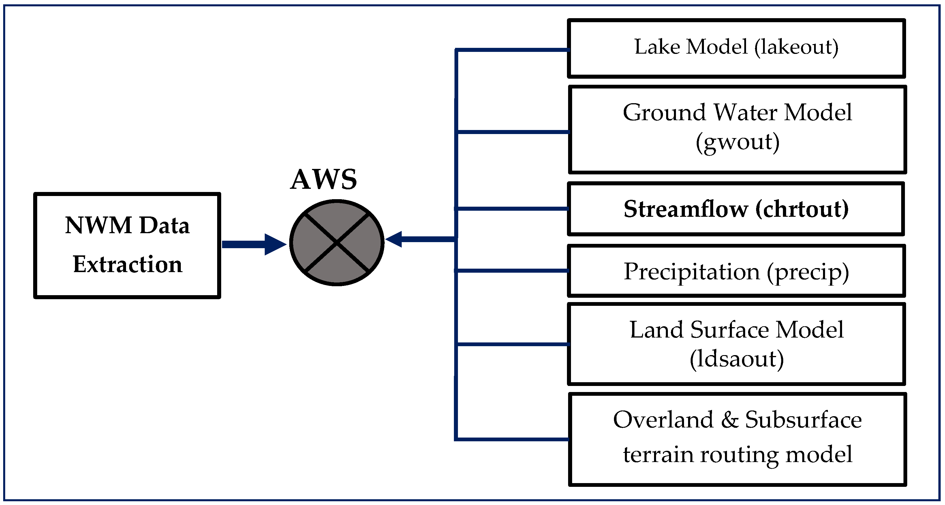
The retrospective dataset from NWM version 2.1 (NWM v2.1) provided the hydrologic baseline that informed the classification thresholds used in the development of AWRI. This dataset, spanning 1 February 1979 to 31 December 2020, was accessed using the guide from NOAA’s official GitHub repository for the NWM retrospective data (https://github.com/NOAA-Big-Data-Program/bdp-data-docs/tree/main/nwm, accessed 10 April 2024). Streamflow variables of interest—“chrtout” in the file format “zarr”—were extracted from the Amazon Web Services (AWS) (Figure 2). The path utilized was s3://noaa-nwm-retrospective-2-1-zarr-pds/chrtout.zarr. While NWM simulates other hydrologic state variables such as soil moisture, streamflow was chosen because it is a critical variable for monitoring water scarcity and excess [10,50,51,52] and provides an operational forecast for hydrologic exposure, capturing both drought and excess scenarios. To characterize hydrological conditions, the research used well established percentile data analysis perspective [46,52,53,54,55,56,57,58].
The USGS classifies streamflow-based water conditions into seven ranges: maximum value, more than 90th percentile, between 76th and 90th percentiles, between 25th and 75th percentiles, between 10th and 24th percentiles, less than 10th percentile, and the minimum value [46]. The United States Drought Monitor (USDM), on the other hand, differentiates between short- and long-term drought conditions. Short-term drought can have impacts on agriculture and grasslands, and the drought classification can rapidly change. Long-term drought, in contrast, has deeper impacts on hydrology and ecology and can persist even with short-term gains in precipitation [52]. Based on these, the research categorized streamflow into nine distinct categories ranging from extreme wetness to exceptional drought conditions.
Stream segment selection was guided by proximity to representative agricultural sites and their associated hydrologic variability. For each selected stream segment (reach ID), streamflow percentiles were calculated for the full retrospective record. This classification system provides the foundation for assigning scores/numerical values that represent exposure to hydrological threats for AWRI scoring. To determine whether stream order influences the representativeness of flow data, a sensitivity analysis was conducted near the agricultural sites on stream orders 2, 5, and 6. The analysis showed minimal differences in streamflow percentiles for orders between 2 and 5, suggesting that lower-order streams may not sufficiently capture hydrological variability. As a result, reach IDs with stream order 6 or higher were prioritized in the AWRI application to ensure stronger spatial representation. Threshold streamflow values defining each hydrological threat category were established for the three finalized Reach IDs used in this study. These thresholds serve as the basis for converting forecasted streamflow values into categorical risk classes as part of the AWRI framework.

2.4. NWM Forecast Retrieval and Preprocessing Pipeline

The operational forecast data from the NWM provided dynamic hydrologic inputs for the real-time risk classification in the AWRI framework. NWM streamflow forecasts are available in three formats: Short range (executed hourly and out to 18 h), medium range (executed every 4 h and extends out to 10 days), and long range (executed every 6 h and extends out to 30 days) [49,59]. Each forecast type includes multiple ensemble members, particularly in the medium and long-range categories. To automate forecast value retrieval, a custom Python 3.11 pipeline was developed. The workflow handled URL construction, file retrieval from NOAA’s NOMADS server, and streamflow extraction for selected reach IDs. For each reach ID used in this study, forecasts were retrieved for the medium and long-range members only. For the medium range, six ensemble members were averaged to obtain a mean series. Similarly, for the long-range forecasts, the averages of four ensemble members were used. For each day, predicted streamflow condition values were later categorized based on the USGS and USDM thresholds defined in Section 2.3, forming the basis for AWRI computation. This pipeline ensured consistent and reproducible use of NWM forecasts, allowing near-real-time agricultural risk assessments at the farm-level for the ABBR.

2.5. Crop Variable Characterization

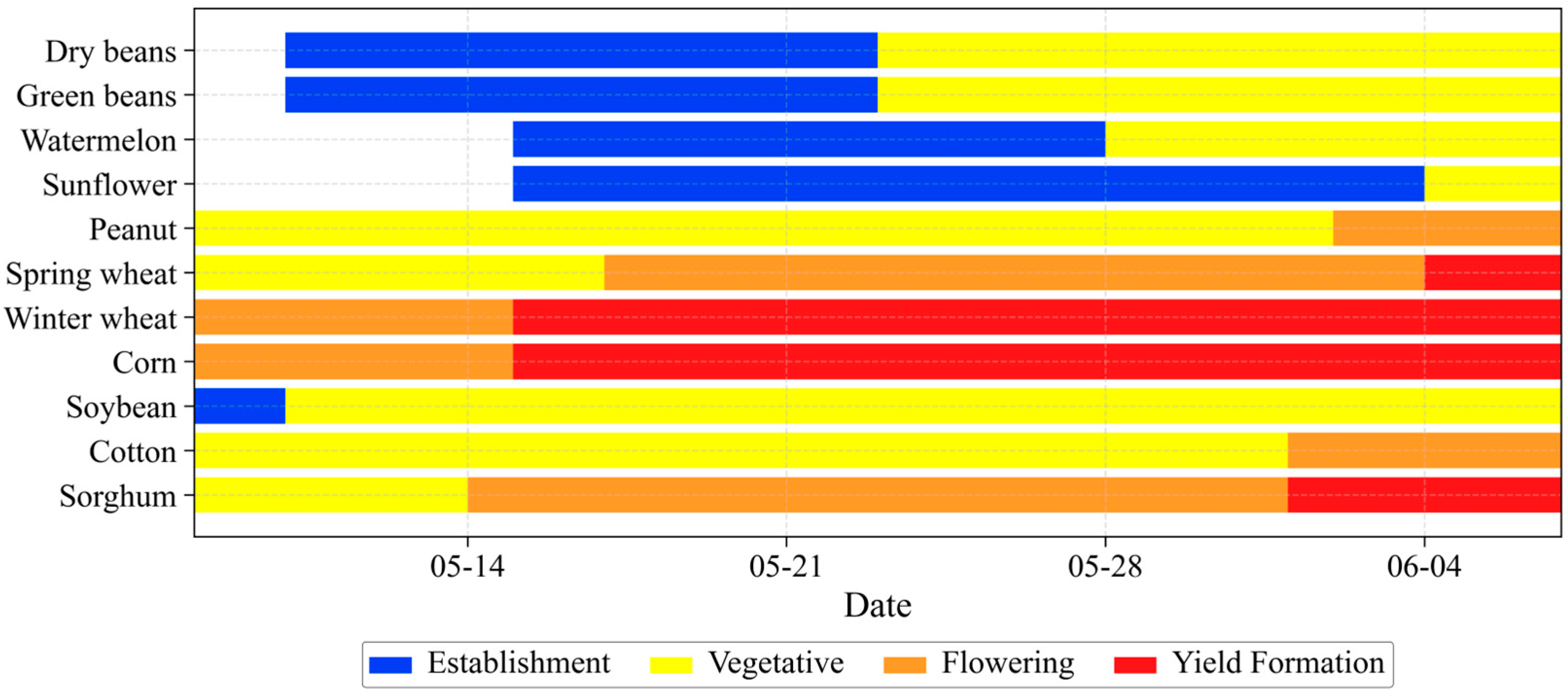
Crop variables reflect the agricultural dimension of water risk in the AWRI framework. This is relative to sensitivity to water stress (scarce and excess) and the adaptive capacity to mitigate such stress. The crop variable integration involved three major components: crop selection, growth stage identification, and tolerance classification. The crop selection process we used in this research was guided by both state and national agricultural data sources. According to [60,61], cotton, soybeans, corn, peanuts, wheat, green beans, dry beans, watermelon, sunflower, and sorghum are the most commonly cultivated crops across Alabama. To localize this selection to the ABBR, cropland cover data from the National Agricultural Statistics Service [62] were spatially analyzed using ArcMap 10.8. to confirm the presence and distribution of these crops in the ABBR. Additionally, we performed crop growth stages mapping using a classification system that included emergence, vegetative growth, flowering, yield formation, and ripening. Each development phase was assigned a standardized stage identifier (ID 0 to ID 4) for consistent integration into the AWRI scoring system. Planting start dates for each crop were aligned with recommendations by [63], allowing the establishment of a crop-specific calendar relevant to the regional climate and management practices. Figure 3 presents the weekly phenological progression of all crops included in this research over the four-week forecast horizon beginning 8 May 2024. For any week in which a crop is not in its active physiological growth, it was labeled “out of season” and excluded from AWRI scoring. Crops were then categorized based on their tolerance to hydrological stress at each growth stage. This classification system follows the assessments described in [64], using three tolerance levels that include high (H), moderate (M), and low (L). These tolerance ratings enabled a more granular sensitivity scoring process. This approach allows crop risk to reflect not just exposure but also biological vulnerability within the AWRI system over time.

2.6. AWRI Framework and Scoring System

The research integrated the NWM streamflow forecast together with information on crop sensitivity or water-stress tolerance, and resilience measures into the AWRI framework. The approach was based on established research on agricultural vulnerability and risk assessment, grounded in three key elements: exposure, sensitivity, and adaptive capacity [10,11,12,18,19,21,65,66,67,68,69]. The AWRI framework was modeled on established vulnerability assessment structures from prior agricultural and environmental studies using an empirical score system [18,21,25].
In this research, the AWRI was computed using the following equation:
AWRI = B1i + B2mn + B3k
B1i: Coefficient for i hydrological threat classification (based on NWM percentiles),
B2mn: Coefficient for tolerance for each m crop to stress condition during n growth stage
B3k: Coefficient for k resilient measures
The AWRI framework uses an additive structure for interpretability, as the components are not equally weighted. The relative influence is governed by coefficient ranges and conditional logic. B1 spans the widest range and always applies, B2 modifies risk based on crop-stage sensitivity, and B3 is activated based on scenarios under hydrologic stress.

2.6.1. Exposure: B1—Coefficient for Hydrological Threat Classification

The B1 coefficient captures the hydrological exposure component of the AWRI, translating forecasted streamflow into a quantitative water-related threat score. The scoring system is based on retrospective streamflow percentiles derived from long-term simulations (1979–2020). This ensures that each classification reflects local hydrology. Based on this, streamflow was classified into nine distinct hydrologic categories, from “Exceptional Drought” to “Extreme Wetness”, based on USGS and USDM percentile classes (Table 1). Each class carries a corresponding B1 empirical score, ranging from −10 for Exceptional Drought to +8 for Extreme Wetness. Normal conditions were centered near zero (−0.1) to reflect agronomic water demand under climatologically neutral conditions. These streamflow categories are designed to reflect real-world agricultural impacts ranging from crop losses to infrastructure damage.
Forecasted streamflow values from the NWM were classified using an automated Python-based pipeline. This system applied percentile thresholds from the historical baseline to ensemble-averaged forecasts across short, medium, and long-range forecasts. For each forecast day, the classification logic determined whether predicted streamflow values fell below the 5th percentile, within the interquartile “normal” range (30th–70th percentile), or exceeded the 90th percentile threshold. To align with weekly crop variables, these daily classifications were aggregated into weekly windows, and the most severe class observed during each week was retained as the final hydrologic threat designation. The corresponding B1 score was then used as the exposure input in the AWRI equation. The use of this percentile-based exposure index aligns with drought and flood classification methodologies in prior agricultural risk literature [21]. This automated classification pipeline served as the operational bridge between NWM forecasts and actionable exposure indicators within the AWRI computation.

2.6.2. Sensitivity: B2—Coefficient for Crop Tolerance to Stress Conditions

The sensitivity component (B2) captures each crop’s tolerance to forecasted hydrological stress at each growth stage [20,21,22,70,71,72,73]. Crops with low tolerance to either water excess or scarcity during critical stages receive the most severe scores (±2), high tolerance crops receive smaller adjustments (±1), and moderate tolerance crops receive (±1.5). Under drought conditions, which is noted as the streamflow value falling below the 30th percentile, B2 scores are assigned negative values to reflect the Water Scarcity condition (S). In contrast, when the streamflow value exceeds the 70th percentile, representing Water Excess conditions (E), B2 values are assigned positive values. For forecasts classified as normal, the value trend for B2 depends on the crop’s stage-specific water requirement. In such scenarios, B2 values are evaluated under both Normal-Water Scarcity and Excess conditions (NS and NE) to capture latent risks. This dual-framing approach under normal hydrologic conditions ensures that agronomic risks are not overlooked. This is especially for sensitive crops like corn or sorghum in active growth stages, where even slight soil moisture imbalances can lead to yield decreases. By incorporating stage-specific tolerance as a sensitivity coefficient, the AWRI accounts for dynamic crop vulnerability. This approach aligns with prior agricultural risk models that emphasize crop-stage specificity [20,22,71,72,73].

2.6.3. Adaptive Capacity: B3—Coefficient for Resilient Measures

The third component of AWRI reflects the farm-level capacity to mitigate risk, and the scoring system in this study uses three possible scenarios. These include the presence of irrigation systems (score: +2.5) to reduce drought impacts and increase resilience, drainage systems (score: −2) to help manage excess water, and the absence of any measure (score: 0) to indicate a scenario of full exposure to the hydrological threat. Accordingly, the B3 score is conditionally applied only when a hydrologic threat is present. This prevents infrastructure presence from independently triggering elevated risk classifications under neutral conditions. These values do not simulate actual water balance impacts on infrastructure but serve to adjust the AWRI classification in a traceable manner. The coefficients, however, allow the AWRI system to account for differences in farmer preparedness and infrastructure access, and hence the final AWRI score. Including this factor is essential because it plays a role in long-term agricultural resilience, building on studies that highlight the role of water infrastructure to mediate agricultural risk under stress conditions [14,21,24].

2.6.4. Composite Classification and Implementation Workflow

To develop and test the AWRI framework, we applied the AWRI (Equation (1)) across selected farm sites, crop types, and forecast periods to assign B1, B2, and B3 scores for specific crop-stage situations. The resulting AWRI values were then categorized into one of eight predefined water risk classes, ranging from “WE-3: Critical Water Excess” to “WS-4: Critical Water Scarcity” (Table 2). These categories translate the numeric output of the AWRI equation into interpretable levels of concern, which are designed to support risk communications.
For instance, an AWRI score of −9 might signal a critical water deficit condition during a crop’s flowering stage, triggering early warning for irrigation planning. Conversely, a positive AWRI of +7 during a vegetative stage might indicate excessive moisture and suggest the need for improved drainage or planting delay. We ensured that the tool specifically addresses hydrological threats while maintaining scalability across diverse agricultural contexts.

3. Results

3.1. Farm-Level Streamflow Mapping for AWRI Evaluation

To evaluate the AWRI tool, a total of five farm locations, with different soil types and hydroclimatic conditions, across the Alabama Black Belt Region, were selected as demonstration sites. However, due to the proximity of some farms and their alignment within shared hydrologic units, the AWRI framework used only three distinct NWM reach IDs. These farms include Brown and Smith in Dallas County, BBMC Selma in Dallas County, and the Blueberry and Tuskegee University organic farm in Macon County. The farms were also selected based on those with installed soil moisture sensors and the availability of research data. Each site was linked to a corresponding NWM reach ID and stream order classification to facilitate forecast-driven hydrologic assessment. Table 3 summarizes the key hydrologic identifiers and their HUC-10 watersheds. Based on preliminary sensitivity and validation analysis (Section 2.3), reach IDs with stream order ≥6 were selected to capture broader hydrologic variability. Each site was assigned crops based on regional agricultural profiles and the top cultivated crops within the ABBR. The crops included corn, soybean, peanut, cotton, sorghum, and winter wheat. These three representative reach IDs were used for all subsequent AWRI computations and scenario applications.

3.2. Streamflow Characterization for B1 Scoring

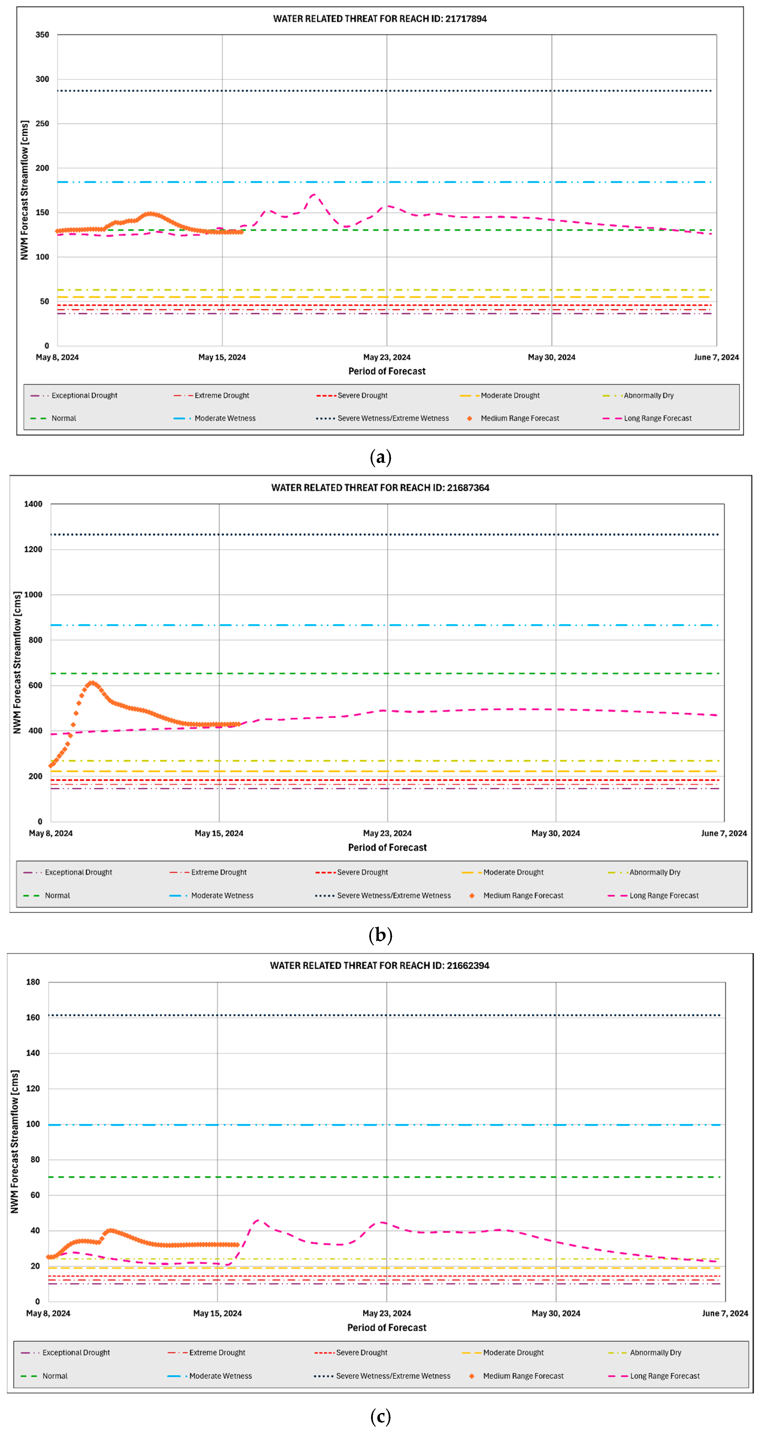
Retrospective streamflow data from the NWM, as described in Section 2.3, were used to establish site-specific percentile thresholds that inform the exposure component (B1) of the AWRI framework. This percentile-based approach ensures that the exposure classification reflects local hydrologic baselines at each farm location. These thresholds, which were tailored individually for reach IDs 21717804, 21687364, and 21662394, served as the reference bins for the transformation of future forecast values into comparable categorical states (Table 4). The resulting thresholds are reach-specific and reflect local stream behavior. For example, the “Extreme Drought” class for reach ID 21687364 begins below 147 cms, whereas for 21717804, it starts below 36 cms. This shows a wide variation across these sites, illustrating the necessity of localized thresholds in any predictive framework. Using these thresholds, forecast streamflow values from the NWM (medium, 8.5 days; long-range, 30 days) were categorized into corresponding hydrological threat classes. Forecast values for this reach were retrieved for 8 May 2024.
A Python-based automation pipeline processed ensemble forecast data and applied the percentile bins to each day’s forecast. For each forecast week, the most severe daily classification was retained as the weekly B1 input for AWRI computation. This approach captures temporal volatility while simplifying cross-comparisons with weekly crop-stage data. The resulting medium and long-range hydrologic threat classifications are summarized in Table 5 and visually represented in Figure 4. For instance, reach ID 21717804 was classified as experiencing “Moderate Wetness” during the first week of the medium-range forecast. In contrast, both reach IDs 21687364 and 21662394 exhibited “Normal” conditions during the same period. By week four, reach ID 21662394 began transitioning toward “Abnormally Dry” conditions in the long-range forecast, while the others remained within normal bounds. These forecast-derived threat labels were converted into B1 scores, providing the first input into the AWRI computation.

3.3. AWRI Scoring Example Across Reach IDs and Forecast Scenarios

To illustrate how the AWRI integrates exposure, sensitivity, and adaptive capacity, we present two worked examples using medium-range forecasts (week 1) issued on 8 May 2024. Weekly crop stages were aligned using the phenology chart (Figure 3), and AWRI scores were calculated according to Equation (1), combining B1 (hydrologic exposure), B2 (crop-stage sensitivity), and B3 (adaptive infrastructure effects) to obtain AWRI classes (Table 2). Eleven crops were simulated across three NWM reach IDs under two management scenarios: with and without field infrastructure (drainage or irrigation). Weekly B2 scores were derived using stage-specific tolerance thresholds from Section 2.6.
Scenario 1: Peanut at Reach ID 21717804, with output shown in Table 6.
Forecast hydrologic condition: Moderate wetness; B1 = +2.0
Crop Stage: Early vegetative (ID1); Low tolerance to water excess; B2 = +2.0
Adaptation Scenarios: Drainage infrastructure will be adequate for the water excess scenario, so for no drainage, B3 = 0; if drainage is present, B3 = −2.0
The presence of drainage substantially reduces the AWRI score, shifting the farm from a water-excess risk zone to a moderate condition.
Scenario 2: Corn at Reach ID 21687364, with output shown in Table 7.
Forecast hydrologic condition: Normal = B1 = −0.1
Crop Stage: Flowering stage (ID2) = Moderate sensitivity to both scarcity and excess, B2 = ±1.5
Adaptation Scenarios: Under normal conditions, AWRI scoring allows for either scarcity or excess framing. Here, drought is emphasized, given corn’s critical water needs during flowering. We considered that if irrigation is applied, B3 = +2.5 and if no infrastructure, B3 = 0
While the crop is moderately sensitive, irrigation increases the AWRI slightly under drought risk framing. However, both interpretations converge around a neutral risk signal, consistent with the streamflow forecast stability.

3.4. AWRI Forecast Outcomes Across Study Sites (Medium and Long Range)

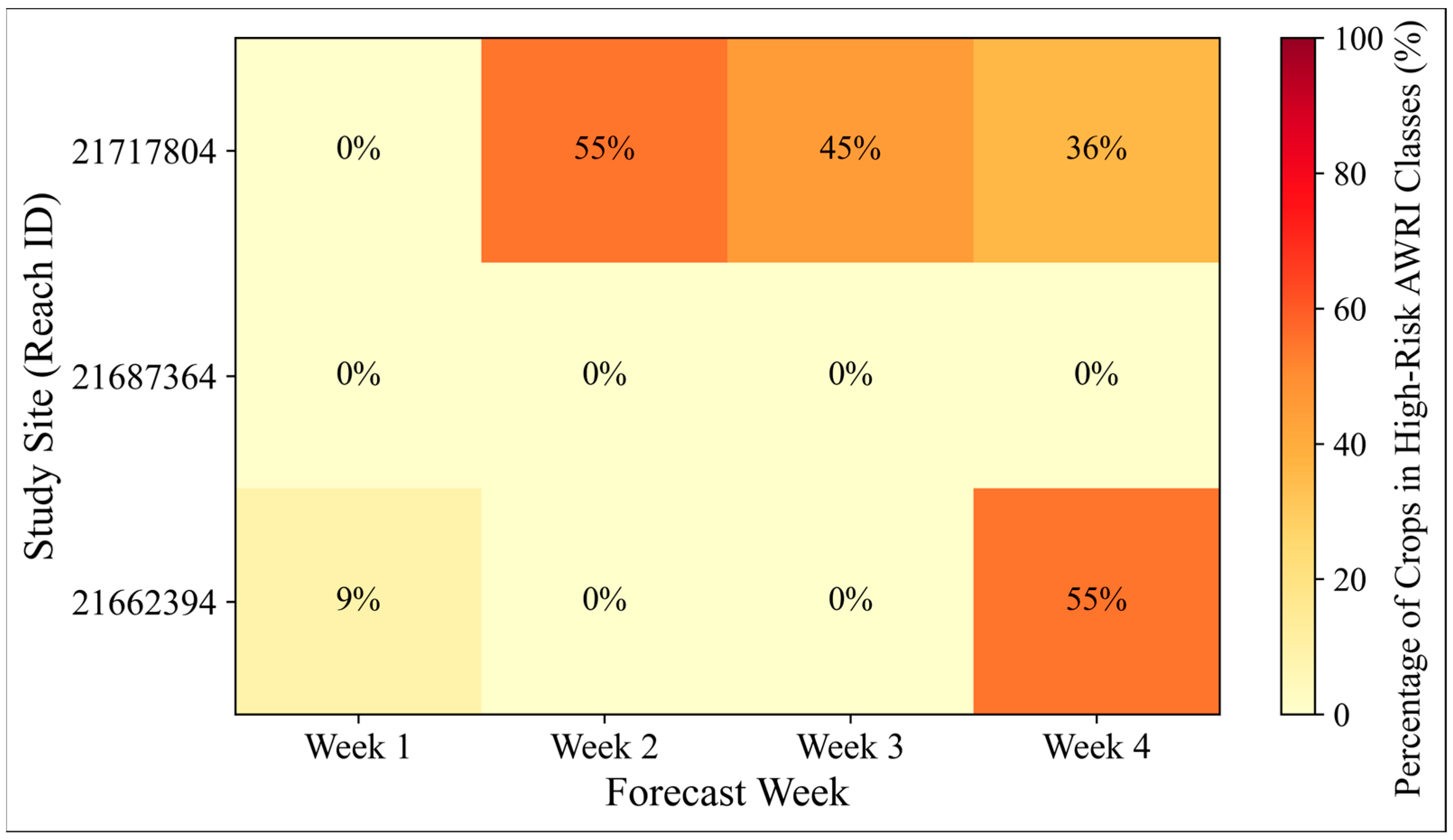
Below are the complete AWRI outputs generated for all three reach IDs across both medium and long-range forecast windows. The scoring logic applied strictly follows the methodology outlined previously, incorporating dynamic B1, B2, and B3 values with AWRI thresholds detailed in Table 2. Table 8, Table 9 and Table 10 summarize the scoring outcomes for long range forecast from 8 May to 6 June 2024. The column headers use the following codes: S = Water Scarcity condition, E = Water Excess condition, NS = Normal-Water Scarcity condition, and NE = Normal-Water Excess condition as described in Section 2.6.2. Figure 5 shows the site-level differences in the percentage of simulated crops (n = 11) classified within high-risk AWRI categories (WS-2, WS-3, WS-4, WE-2, WE-3) under scenarios without resilience measures.

3.4.1. Reach ID 21717804 (Blueberry Farm and Tuskegee University Organic Farm)

From Table 8, this site consistently experienced forecasted moderate wetness during the first week in the medium-range forecast and hovered near the normal-to-moderate wetness threshold under long-range forecasts. As a result, water excess emerged as the primary hydrologic threat across most crops, particularly during the early stages (ID0–ID2), where sensitivity to excess is highest. Without drainage, AWRI scores for crops such as dry beans, green beans, peanuts, cotton, and sorghum frequently reached +3.5 to +4.0, triggering WE-2 (Severe Water Excess) classifications. When drainage infrastructure was simulated (B3 = −2.0), most risk scores dropped to the +1.5 to +2.0 range, shifting crops into WE-1 (moderate water excess) and even WN-0 (Normal). These results illustrate the role of drainage infrastructure in reducing risks related to water excess, especially during early vegetative periods when crop tolerance is limited. Additionally, as noted in Section 2.6.2, week 1 captured both the NS and NE columns to reflect crop sensitivity at specific growth stages under normal streamflow conditions. For example, winter wheat was at the flowering stage, indicating a period of high vulnerability to scarcity.

3.4.2. Reach ID 21687364 (Brown and Smith Farm)

From Table 9, it is observed that forecast conditions for this site remained consistently normal across both forecast ranges. Given the neutral hydrologic input (B1 = −0.1), AWRI scores were driven primarily by crop sensitivity (B2). Both excess and drought risk framings were tested under normal conditions, with most AWRI scores ranging from +1.6 to −1.6, retaining the WN-0 (Normal) band. However, crops such as wheat, corn, and peanuts were classified as abnormally dry (WS-1) in the AWRI classification. This aligns with the fact that these crops were at a level that reflects their elevated moisture demand. With irrigation infrastructure assumed (B3 = +2.5), the drought risk framing shifted some crops upward slightly, but not beyond the normal threshold. This site reinforced the AWRI framework’s ability to maintain scoring neutrality when conditions are stable, while still flagging vulnerability in key crop stages.

3.4.3. Reach ID 21662394 (BBMC Selma Farm)

This site, as shown in Table 10, exhibited mild variability across forecast windows, with some long-range predictions dipping into abnormally dry conditions during weeks 1 and 4. As a result, water scarcity emerged as the primary hydrologic threat across these crops. This pushed B1 values downward, to amplify water scarcity risk for crops in critical reproductive stages. Crops such as corn, dry bean, green bean, spring wheat, and watermelon scored AWRI values between −2.5 and −3.0 during dry weeks without irrigation, triggering WS-2 (moderate water scarcity) and WS-1 (abnormally dry) classes. Assumed irrigation infrastructure shifted these values upward by +2.5 points, often bringing AWRI scores back into the WS-1 or WN-0 range, which demonstrates the tool’s capacity to capture mitigation potential. However, during weeks 2 to 3, crops remained mostly within normal or mildly dry classes even in the absence of irrigation. This case highlights the AWRI framework’s responsiveness to week-to-week hydrologic fluctuations and stage-specific crop demands.
As shown in Figure 5, Reach ID 21717804 exhibited the highest proportion of simulated crops exposed to high-risk AWRI classes, particularly during Week 2 (55%) and Week 3 (45%). For Reach ID 21662394, risk spikes were most evident in Week 4 (55%), aligning with simulated drought threats and crop water demand phases. In contrast, Reach ID 21687364 maintained zero high-risk exposure across all weeks, reinforcing the neutral conditions observed in Table 9. These differences underscore AWRI’s temporal precision and site-specific responsiveness.

4. Discussion

The application of the AWRI framework across research reaches and farm sites in the Alabama Black Belt Region demonstrated its capability to resolve location-specific, crop-sensitive, and infrastructure-adjusted risk classification using NWM forecast data. The scoring system’s integration of B1 (exposure), B2 (sensitivity), and B3 (adaptive capacity) components allowed the framework to distinguish not only between drought and excess conditions but also to contextualize risk severity to crop phenology. Across the reach IDs, forecast conditions ranged from moderate wetness to abnormally dry, with implications that shifted weekly depending on both the hydrologic outlook and the crop growth stage. These trends are further visualized in Figure 5, which shows that site-specific risk exposure varied sharply over the forecast period. For instance, reach ID 21717804 consistently signaled severe water excess conditions for several crops in early vegetative stages, an outcome that was significantly reduced when drainage was hypothetically assumed. Meanwhile, reach ID 21662394 revealed drought-related risk transitions in the forecast window. In contrast, the stability observed at reach ID 21687364 underscored that AWRI does not produce false alarms under neutral conditions. This reinforces its reliability as a practical early warning tool. Across all evaluated reach IDs, two consistent trends were evident. First, infrastructure measures (drainage or irrigation) reduced risk classifications by one to two levels in most scenarios, confirming their protective role. Second, crops in vegetative or reproductive stages showed the greatest sensitivity to hydrologic stress, making timing a critical dimension in risk forecasting. This aligns with prior findings that emphasized the effectiveness of targeted water infrastructure [18,19,21]. The AWRI’s quantitative structure allowed these dynamics to be validated across both medium- and long-range forecast scenarios.
Specifically, one of the AWRI’s strengths lies in its temporal precision. By assigning weekly B2 sensitivity scores, the framework captured not just the intensity of water stress, but its timing in relation to crop development. This is a key dimension often overlooked by static indices. Meanwhile, the B3 coefficient enabled simulation of infrastructure benefits, turning adaptive capacity from a background variable into a measurable influence on risk. These results confirm the AWRI’s capability to assess exposure and sensitivity with high resolution to support farm-scale decisions. With forecast windows ranging from 1 to 4 weeks, farmers and landowners are positioned to anticipate water-related threats and take proactive management practices. While the AWRI framework translates hydrologic exposure and crop-stage sensitivity into operationally useful risk scores, direct evaluation against observed yield losses was not conducted in this study. Nonetheless, future iterations of AWRI would include evaluation against field-level yield trends, farmer-reported damage events, remote sensing products, and modeled crop response outputs. Such validation would enhance the tool as a decision-support tool for both monitoring and mitigation.

5. Conclusions

This study developed and implemented an AWRI framework that uses a scoring system to quantify hydrologic threats to crop variables based on forecasted streamflow data from the NWM. Using reach IDs from the NWM, specific to research farm sites, the AWRI demonstrated its ability to translate raw hydrologic predictions into actionable risk classes across diverse crop and management scenarios. A key strength of the framework is its temporal precision. The AWRI dynamically adjusts risk scores in response to evolving streamflow forecasts and changing crop sensitivity. This enables more accurate identification of water-risk windows. As the examples presented demonstrate, including infrastructure scenarios enhances the tool’s practical relevance by showing users how drainage or irrigation may alter the risk profile in real time. While the current coefficient system allows traceable scoring logic, future work would involve sensitivity analysis of B2 and B3 values to improve empirical grounding. By focusing on dynamic risk profiles, the AWRI serves as a practical bridge between hydrologic forecasting systems and farm-level decision support systems. Possible seasonal shifts also underscore the importance of future tools that can integrate AWRI logic with ensemble climate data to support adaptive water management under evolving local hydrology. Future extensions may incorporate ensemble forecast variability, finer-resolution field data, soil moisture products, economic cost component, or crop yield modeling to refine risk projections and improve spatial relevance at farm scales. The AWRI currently stands as a scalable tool for water-related agricultural risk management guidance for farmers, land managers, and decision-makers across diverse agricultural landscapes. To enhance accessibility and facilitate practical use, future work would focus on translating the AWRI framework into a spatial dashboard interface. This platform could visualize forecast-based risk scores, offering real-time decision support tailored to site-specific agricultural management.

Author Contributions

Conceptualization, J.E.Q. and R.G.D.; methodology, J.E.Q. and R.G.D.; formal analysis, R.G.D., E.E.O. and J.E.Q.; investigation, J.E.Q.; resources, J.E.Q.; writing—original draft, R.G.D., E.E.O. and J.E.Q.; writing—review and editing, J.E.Q., R.G.D., E.E.O. and S.F.; supervision, J.E.Q. and S.F.; funding acquisition, J.E.Q. All authors have read and agreed to the published version of the manuscript.

Funding

This research was funded by the Cooperative Institute for Research to Operations in Hydrology (CIROH) under award NA22NWS4320003 from the NOAA Cooperative Institute Program. The statements, findings, conclusions, and recommendations are those of the authors and do not necessarily reflect the opinions of NOAA.

Data Availability Statement

The NWM retrospective data used in the study was extracted using the guidelines of the official GitHub repository of the NOAA NWM Retrospective Model Data (https://github.com/NOAA-Big-Data-Program/bdp-data-docs/tree/main/nwm, accessed on 20 January 2026). The extraction process utilized the Amazon Web Services (AWS) cloud repository. The path utilized was s3://noaa-nwm-retrospective-2-1-zarr-pds/chrtout.zarr, accessed 10 April 2024. Reach IDs for each stream of interest are available via the NWM web map (https://water.noaa.gov/map, accessed 10 April 2024). AWRI Python scripts, database, and tools are available in the repository at Tuskegee University Geospatial Center and CIROH.

Conflicts of Interest

All authors declare that the research was conducted in the absence of any commercial or financial relationships that could be construed as a potential conflict of interest.

Abbreviations

The following abbreviations are used in this manuscript:
ABBRAlabama Black Belt Region
AWRIAgricultural Water Risk Indicator
HANDHeight Above Nearest Drainage
HRRRHigh-Resolution Rapid Refresh
LSMLand Surface Model
MPEMultisensor Precipitation Estimator
MRMSMulti-Radar/Multi-Sensor System
NAM-NESTNorth American Mesoscale Nest
NCARNational Center for Atmospheric Research
NHDNational Hydrography Dataset
NOAANational Oceanic and Atmospheric Administration
NSEThe Nash–Sutcliffe Model Efficiency Coefficient
NWMNational Water Model
NWPNumerical Weather Prediction
OARCOffice of Water Prediction Analysis of Record for Calibration
PBIASPercent Bias
RAPRapid Refresh
RSRMean Square Error Observation Standard Deviation Ratio
USDMUnited States Drought Monitor
WRF-HydroWater Research and Forecasting Hydrological Model

References

  1. Choi, E.; Rigden, A.J.; Tangdamrongsub, N.; Jasinski, M.F.; Mueller, N.D. US crop yield losses from hydroclimatic hazards. Environ. Res. Lett. 2023, 19, 014005. [Google Scholar] [CrossRef]
  2. Rupngam, T.; Messiga, A.J. Unraveling the Interactions between Flooding Dynamics and Agricultural Productivity in a Changing Climate. Sustainability 2024, 16, 6141. [Google Scholar] [CrossRef]
  3. Zhou, Q.; Leng, G.; Peng, J. Recent Changes in the Occurrences and Damages of Floods and Droughts in the United States. Water 2018, 10, 1109. [Google Scholar] [CrossRef]
  4. Kuwayama, Y.; Thompson, A.; Bernknopf, R.; Zaitchik, B.; Vail, P. Estimating the impact of drought on agriculture using the US Drought Monitor. Am. J. Agric. Econ. 2019, 101, 193–210. [Google Scholar] [CrossRef]
  5. Rodziewicz, D.; Dice, J. Drought Risk to the Agriculture Sector. Econ. Rev. 2020, 105, 61–86. [Google Scholar] [CrossRef]
  6. Tanir, T.; Yildirim, E.; Ferreira, C.M.; Demir, I. Social vulnerability and climate risk assessment for agricultural communities in the United States. Sci. Total. Environ. 2023, 908, 168346. [Google Scholar] [CrossRef]
  7. Mabhaudhi, T.; Dirwai, T.L.; Taguta, C.; Sikka, A.; Lautze, J. Mapping Decision Support Tools (DSTs) on agricultural water productivity: A global systematic scoping review. Agric. Water Manag. 2023, 290, 108590. [Google Scholar] [CrossRef]
  8. Ahsan, M.N.; Warner, J. The socioeconomic vulnerability index: A pragmatic approach for assessing climate change led risks–A case study in the south-western coastal Bangladesh. Int. J. Disaster Risk Reduct. 2014, 8, 32–49. [Google Scholar] [CrossRef]
  9. Rey, D.; Garrido, A.; Calatrava, J. Comparison of different water supply risk management tools for irrigators: Option contracts and insurance. Environ. Resour. Econ. 2015, 65, 415–439. [Google Scholar] [CrossRef]
  10. Collet, L.; Beevers, L.; Stewart, M.D. Decision-making and flood risk uncertainty: Statistical data set analysis for flood risk assessment. Water Resour. Res. 2018, 54, 7291–7308. [Google Scholar] [CrossRef]
  11. Kodama, C.; Stevens, B.; Mauritsen, T.; Seiki, T.; Satoh, M. A new perspective for future precipitation change from intense extratropical cyclones. Geophys. Res. Lett. 2019, 46, 12435–12444. [Google Scholar] [CrossRef]
  12. Scherrer, S.C.; Fischer, E.M.; Posselt, R.; Liniger, M.A.; Croci-Maspoli, M.; Knutti, R. Emerging trends in heavy precipitation and hot temperature extremes in Switzerland. J. Geophys. Res. Atmos. 2016, 121, 2626–2637. [Google Scholar] [CrossRef]
  13. Wilkinson, M.E.; Quinn, P.F.; Hewett, C.J. The Floods and Agriculture Risk Matrix: A decision support tool for effectively communicating flood risk from farmed landscapes. Int. J. River Basin Manag. 2013, 11, 237–252. [Google Scholar] [CrossRef]
  14. Fadul, E.; Masih, I.; De Fraiture, C. Adaptation strategies to cope with low, high and untimely floods: Lessons from the Gash spate irrigation system, Sudan. Agric. Water Manag. 2019, 217, 212–225. [Google Scholar] [CrossRef]
  15. Sharma, V.; Irmak, A.; Kabenge, I.; Irmak, S. Application of GIS and geographically weighted regression to evaluate the spatial non-stationarity relationships between precipitation vs. irrigated and rainfed maize and soybean yields. Trans. ASABE 2011, 54, 953–972. [Google Scholar] [CrossRef]
  16. Corral-Quintana, S.; la Nuez, D.L.-D.; Verna, C.L.; Hernández, J.H.; de Lara, D.R.-M. How to improve strategic decision-making in complex systems when only qualitative information is available. Land Use Policy 2016, 50, 83–101. [Google Scholar] [CrossRef]
  17. Zarghami, M. Effective watershed management; Case study of Urmia Lake, Iran. Lake Reserv. Manag. 2011, 27, 87–94. [Google Scholar] [CrossRef]
  18. Azmi, M.; Rüdiger, C.; Walker, J.P. A data fusion-based drought index. Water Resour. Res. 2016, 52, 2222–2239. [Google Scholar] [CrossRef]
  19. Murthy, C.; Laxman, B.; Sai, M.S. Geospatial analysis of agricultural drought vulnerability using a composite index based on exposure, sensitivity and adaptive capacity. Int. J. Disaster Risk Reduct. 2015, 12, 163–171. [Google Scholar] [CrossRef]
  20. Cui, Y.; Jiang, S.; Jin, J.; Ning, S.; Feng, P. Quantitative assessment of soybean drought loss sensitivity at different growth stages based on S-shaped damage curve. Agric. Water Manag. 2019, 213, 821–832. [Google Scholar] [CrossRef]
  21. Sehgal, V.K.; Dhakar, R. Geospatial approach for assessment of biophysical vulnerability to agricultural drought and its intra-seasonal variations. Environ. Monit. Assess. 2016, 188, 197. [Google Scholar] [CrossRef]
  22. Pei, W.; Fu, Q.; Liu, D.; Li, T.; Cheng, K.; Cui, S. A novel method for agricultural drought risk assessment. Water Resour. Manag. 2019, 33, 2033–2047. [Google Scholar] [CrossRef]
  23. Scheumann, W.; Freisem, C. The role of drainage for sustainable agriculture. J. Appl. Irrig. Sci. 2002, 37, 33–61. [Google Scholar]
  24. Ritzema, H. Drain for Gain: Managing salinity in irrigated lands—A review. Agric. Water Manag. 2016, 176, 18–28. [Google Scholar] [CrossRef]
  25. Turner, B.L., II; Kasperson, R.E.; Matson, P.A.; McCarthy, J.J.; Corell, R.W.; Christensen, L.; Eckley, N.; Kasperson, J.X.; Luers, A.; Martello, M.L.; et al. A framework for vulnerability analysis in sustainability science. Proc. Natl. Acad. Sci. USA 2003, 100, 8074–8079. [Google Scholar] [CrossRef]
  26. Li, X.; Zhang, C.; Huo, Z. Optimizing irrigation and drainage by considering agricultural hydrological process in arid farmland with shallow groundwater. J. Hydrol. 2020, 585, 124785. [Google Scholar] [CrossRef]
  27. Playán, E.; Mateos, L. Modernization and optimization of irrigation systems to increase water productivity. Agric. Water Manag. 2006, 80, 100–116. [Google Scholar] [CrossRef]
  28. Jackson, T.; Hanjra, M.A.; Khan, S.; Hafeez, M. Building a climate resilient farm: A risk based approach for understanding water, energy and emissions in irrigated agriculture. Agric. Syst. 2011, 104, 729–745. [Google Scholar] [CrossRef]
  29. Dizaj, A.A.; Noory, H.; Ebrahimian, H. Effect of irrigation depth reduction, planting date and cropping pattern on water productivity in West Lake Urmia, Iran. Irrig. Drain. 2018, 68, 191–204. [Google Scholar] [CrossRef]
  30. Bales, J.; Flowers, T. Featured Collection Introduction: National Water Model IV. J. Am. Water Resour. Assoc. 2022, 58, 767–769. [Google Scholar] [CrossRef]
  31. Quansah, J.; Doria, R.; Fall, S. Evaluating the Performance of the National Water Model: A Spatiotemporal Analysis of Streamflow Forecasting. Water 2025, 17, 2950. [Google Scholar] [CrossRef]
  32. NOAA. The National Water Model; OWP Office of Water Prediction: Washington, DC, USA, 2023. Available online: https://water.noaa.gov/about/nwm (accessed on 22 October 2025).
  33. Jachens, E.; Hutcheson, H.; Thomas, M. Groundwater-Surface Water Exchange and Streamflow Prediction using the National Water Model in the Northern High Plains Aquifer region, USA. In National Water Center Innovators Program Summer Institute Report 2018; Columbia Engineering: New York, NY, USA, 2018. [Google Scholar]
  34. Kopp, S.; Cline, D.; Miniat, C.; Lucero, C.; Rothlisberger, J.; Levinson, D.; Evett, S.; Brusberg, M.; Lowenfish, M.; Strobel, M.; et al. Perspectives on the National Water Model. AWRA Impact 2018, 20, 10–11. [Google Scholar]
  35. Shastry, A.; Egbert, R.; Aristizabal, F.; Luo, C.; Yu, C.; Praskievicz, S. Using steady-state backwater analysis to predict inundated area from National Water Model streamflow simulations. JAWRA J. Am. Water Resour. Assoc. 2019, 55, 940–951. [Google Scholar] [CrossRef]
  36. Johnson, J.M.; Munasinghe, D.; Eyelade, D.; Cohen, S. An integrated evaluation of the National Water Model (NWM)–Height Above Nearest Drainage (HAND) flood mapping methodology. Nat. Hazards Earth Syst. Sci. 2019, 19, 2405–2420. [Google Scholar] [CrossRef]
  37. Viterbo, F.; Mahoney, K.; Read, L.; Salas, F.; Bates, B.; Elliott, J.; Cosgrove, B.; Dugger, A.; Gochis, D.; Cifelli, R. A multiscale, hydrometeorological forecast evaluation of National Water Model forecasts of the May 2018 Ellicott City, Maryland, flood. J. Hydrometeorol. 2020, 21, 475–499. [Google Scholar] [CrossRef]
  38. Zheng, X.; D’Angelo, C.; Maidment, D.R.; Passalacqua, P. Application of a large-scale terrain-analysis-based flood mapping system to Hurricane Harvey. J. Am. Water Resour. Assoc. 2022, 58, 149–163. [Google Scholar] [CrossRef]
  39. Duan, Y.; Kumar, S. Predictability of seasonal streamflow and soil moisture in National Water Model and a humid Alabama-Coosa-Tallapoosa River Basin. J. Hydrometeorol. 2020, 21, 1447–1467. [Google Scholar] [CrossRef]
  40. Raczynski, K.; Dyer, J. Variability of annual and monthly streamflow droughts over the southeastern United States. Water 2022, 14, 3848. [Google Scholar] [CrossRef]
  41. S.1643-117th Congress (2021–2022): Alabama Black Belt National Heritage Area Act (2021-05-13). Available online: https://www.congress.gov/bill/117th-congress/senate-bill/1643 (accessed on 22 October 2025).
  42. Smith, E.A.; Johnson, L.C.; Langdon, D.W., Jr.; Aldrich, T.H.; Cunningham, K.M. Report on the Geology of the Coastal Plain of Alabama; Special Report 6; Brown Printing Company, State Printers: Monterey Park, CA, USA, 1894; p. 759. Available online: https://books.google.com/books?id=BzsxAQAAMAAJ&printsec=frontcover&source=gbs_ge_summary_r&cad=0#v=onepage&q&f=false (accessed on 22 October 2025).
  43. Stephenson, L.W.; Monrow, W.H. Stratigraphy of the Upper Cretaceous series in Mississippi and Alabama; Bulletin V. 22 12; American Association of Petroleum Geologists: Tulsa, OK, USA, 1938; pp. 1639. Available online: https://ngmdb.usgs.gov/Prodesc/proddesc_87938.htm (accessed on 22 October 2025).
  44. Winemiller, T. Black Belt Region in Alabama. In Encyclopedia of Alabama; Alabama Humanities Alliance: Birmingham, AL, USA, 2009; Available online: https://encyclopediaofalabama.org/article/black-belt-region-in-alabama/ (accessed on 22 October 2025).
  45. USGS. Hydrologic Unit Codes (HUCs) Explained; USGS: Reston, VA, USA, 2024. Available online: https://nas.er.usgs.gov/about/hucs.aspx (accessed on 22 October 2025).
  46. USGS. USGS Current Water Data for the Nation. 2024. Available online: https://waterdata.usgs.gov/nwis/rt (accessed on 10 April 2024).
  47. NOAA. National Water Model. Available online: https://toolkit.climate.gov/tool/national-water-model (accessed on 22 October 2025).
  48. Gochis, D.J.; Cosgrove, B.; Dugger, A.L.; Karsten, L.; Sampson, K.M.; McCreight, J.L.; Flowers, T.; Clark, E.P.; Vukicevic, T.; Salas, F.; et al. Multi-Variate Evaluation of the NOAA National Water Model; H33G-01; AGU Fall Meeting Abstracts; American Geophysical Union: Washington, DC, USA, 2018. Available online: https://ui.adsabs.harvard.edu/abs/2018AGUFM.H33G..01G/abstract (accessed on 22 October 2025).
  49. Cosgrove, B.; Gochis, D.; Flowers, T.; Dugger, A.; Ogden, F.; Graziano, T.; Clark, E.; Cabell, R.; Casiday, N.; Cui, Z.; et al. NOAA’s National Water Model: Advancing operational hydrology through continental-scale modeling. JAWRA J. Am. Water Resour. Assoc. 2024, 60, 247–272. [Google Scholar] [CrossRef]
  50. Haslinger, K.; Koffler, D.; Schöner, W.; Laaha, G. Exploring the link between meteorological drought and streamflow: Effects of climate-catchment interaction. Water Resour. Res. 2014, 50, 2468–2487. [Google Scholar] [CrossRef]
  51. Álvarez-Berríos, N.L.; Soto-Bayó, S.; Holupchinski, E.; Fain, S.J.; Gould, W.A. Correlating drought conservation practices and drought vulnerability in a tropical agricultural system. Renew. Agric. Food Syst. 2018, 33, 279–291. [Google Scholar] [CrossRef]
  52. National Drought Mitigation Center. What is the US Drought Monitor. United States Drought Monitor. 2024. Available online: https://droughtmonitor.unl.edu/About/WhatistheUSDM.aspx (accessed on 18 May 2024).
  53. Auer, I.; Böhm, R. Combined temperature-precipitation variations in Austria during the instrumental period. Theor. Appl. Clim. 1994, 49, 161–174. [Google Scholar] [CrossRef]
  54. Chmielewski, F.-M.; Potts, J. The relationship between crop yields from an experiment in southern England and long-term climate variations. Agric. For. Meteorol. 1995, 73, 43–66. [Google Scholar] [CrossRef]
  55. Hansen, C.; Shiva, J.S.; McDonald, S.; Nabors, A. Assessing Retrospective National Water Model Streamflow with Respect to Droughts and Low Flows in the Colorado River Basin. JAWRA J. Am. Water Resour. Assoc. 2019, 55, 964–975. [Google Scholar] [CrossRef]
  56. Kothari, K.; Ale, S.; Bordovsky, J.P.; Thorp, K.R.; Porter, D.O.; Munster, C.L. Simulation of efficient irrigation management strategies for grain sorghum production over different climate variability classes. Agric. Syst. 2019, 170, 49–62. [Google Scholar] [CrossRef]
  57. Lins, H.F.; Slack, J.R. Seasonal and Regional Characteristics of U.S. Streamflow Trends in the United States from 1940 to 1999. Phys. Geogr. 2005, 26, 489–501. [Google Scholar] [CrossRef]
  58. Luce, C.H.; Holden, Z.A. Declining annual streamflow distributions in the Pacific Northwest United States, 1948–2006. Geophys. Res. Lett. 2009, 36, L16401. [Google Scholar] [CrossRef]
  59. Ames, D. Introduction to the National Water Model. Hydrolearn. 2020. Available online: https://apps.edx.hydrolearn.org/learning/course/course-v1:BYU+NWM101+2021/home (accessed on 20 March 2024).
  60. USDA. 2022 Census of Agriculture: Alabama, State and County Data (AC-22-A-1, p. 741). United States Department of Agriculture. 2024. Available online: https://www.nass.usda.gov/Publications/AgCensus/2022/Full_Report/Volume_1,_Chapter_1_State_Level/Alabama/alv1.pdf (accessed on 12 April 2024).
  61. Alabama Department of Agriculture and Industries. Alabama Agricultural Facts (p. 2). United States Department of Agriculture. 2022. Available online: https://www.nass.usda.gov/Statistics_by_State/Alabama/Publications/More_Features/ALAgFacts.pdf (accessed on 12 April 2024).
  62. National Agricultural Statistic Service (NASS). CropScape—NASS CDL Program. 2022. Available online: https://nassgeodata.gmu.edu/CropScape/ (accessed on 12 April 2024).
  63. USDA; NASS. Usual Planting and Harvesting Dates for U.S. Field Crops; Agricultural Handbook 628; United States Department of Agriculture: Washington, DC, USA, 1997; p. 51. Available online: https://swat.tamu.edu/media/90113/crops-typicalplanting-harvestingdates-by-states.pdf (accessed on 12 April 2024).
  64. Boguszewska-Mańkowska, D.; Ruszczak, B.; Zarzyńska, K. Classification of potato varieties drought stress tolerance using supervised learning. Appl. Sci. 2022, 12, 1939. [Google Scholar] [CrossRef]
  65. Brackins, J.T.; Kalyanapu, A.J. Using ADCIRC and HEC-FIA Modeling to Predict Storm Surge Impact on Coastal Infrastructure. In Proceedings of the World Environmental and Water Resources Congress, West Palm Beach, FL, USA, 22–26 May 2016; pp. 203–212. [Google Scholar]
  66. García-León, D.; Contreras, S.; Hunink, J. Comparison of meteorological and satellite-based drought indices as yield predictors of Spanish cereals. Agric. Water Manag. 2019, 213, 388–396. [Google Scholar] [CrossRef]
  67. Mokhtari, F.; Soltani, S.; Mousavi, S.A. Assessment of Flood Damage on Humans, Infrastructure, and Agriculture in the Ghamsar Watershed Using HEC-FIA Software. Nat. Hazards Rev. 2017, 18, 04017006. [Google Scholar] [CrossRef]
  68. Sidek, L.M.; Yalit, M.R.; Djuladi, D.A.; Marufuzzaman, M. Flood Damage Assessment for Pergau Hydroelectric Power Project using HEC-FIA. IOP Conf. Ser. Earth Environ. Sci. 2021, 704, 012002. [Google Scholar] [CrossRef]
  69. Todisco, F.; Vergni, L.; Mannocchi, F. Operative Approach to Agricultural Drought Risk Management. J. Irrig. Drain. Eng. 2009, 135, 654–664. [Google Scholar] [CrossRef]
  70. Gobin, A. Weather related risks in Belgian arable agriculture. Agric. Syst. 2018, 159, 225–236. [Google Scholar] [CrossRef]
  71. Valverde-Arias, O.; Garrido, A.; Valencia, J.L.; Tarquis, A.M. Using geographical information system to generate a drought risk map for rice cultivation: Case study in Babahoyo canton (Ecuador). Biosyst. Eng. 2018, 168, 26–41. [Google Scholar] [CrossRef]
  72. Wei, Y.; Jin, J.; Jiang, S.; Ning, S.; Cui, Y.; Zhou, Y. Simulated Assessment of Summer Maize Drought Loss Sensitivity in Huaibei Plain, China. Agronomy 2019, 9, 78. [Google Scholar] [CrossRef]
  73. Xu, H.; Tian, Z.; He, X.; Wang, J.; Sun, L.; Fischer, G.; Fan, D.; Zhong, H.; Wu, W.; Pope, E.; et al. Future increases in irrigation water requirement challenge the water-food nexus in the northeast farming region of China. Agric. Water Manag. 2019, 213, 594–604. [Google Scholar] [CrossRef]
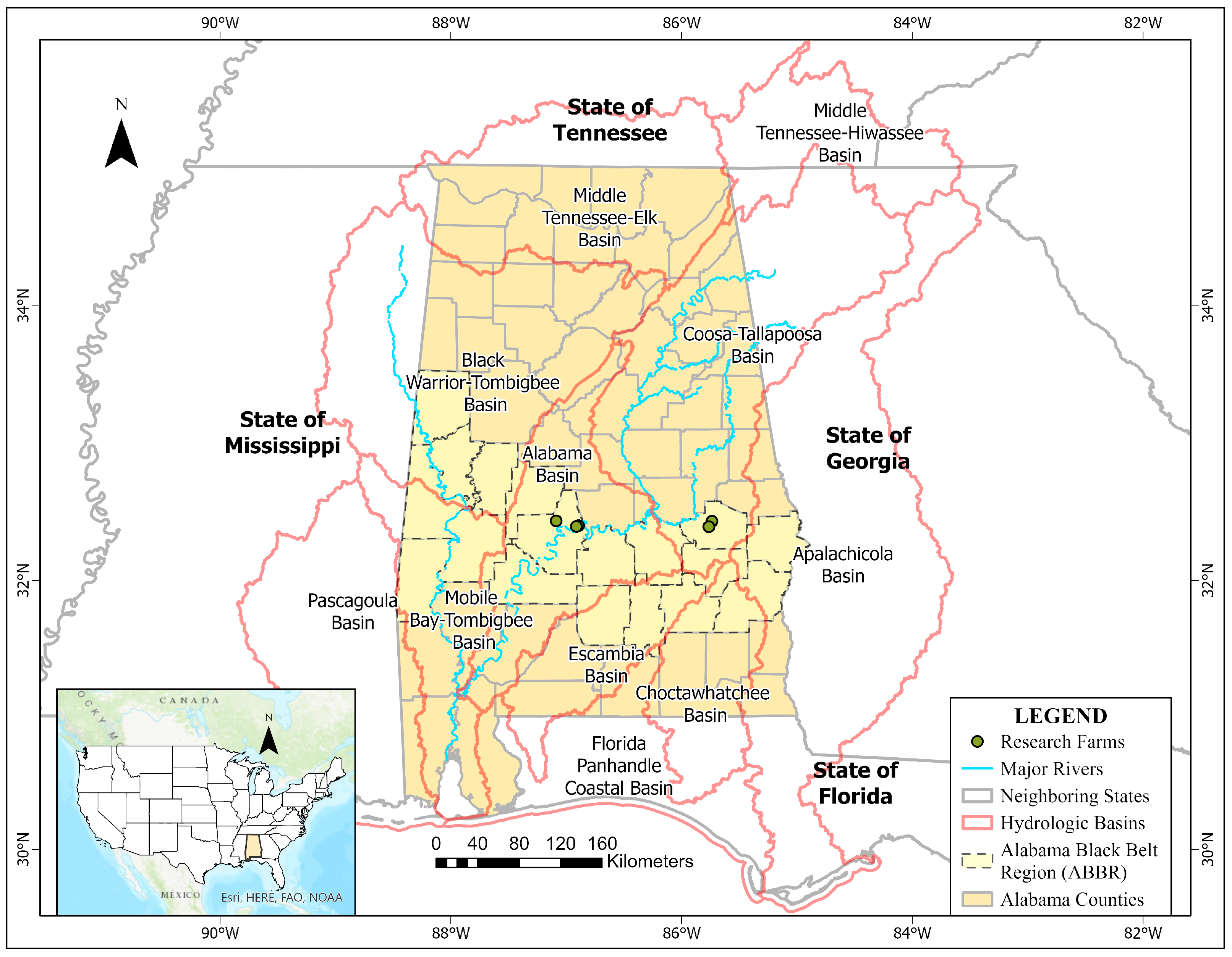
Figure 1. The state of Alabama highlighting the ABBR counties and their hydrologic basins.
Hydrology 13 00043 g001
Figure 2. The NWM data extraction method via Amazon Web Services.
Hydrology 13 00043 g002
Figure 3. Crop growth stages and timeline from 8 May to 6 June 2024.
Hydrology 13 00043 g003
Figure 4. NWM Forecast and threat assessment for reach IDs: (a) 21717804, (b) 21687364, and (c) 21662394.
Hydrology 13 00043 g004
Figure 5. Percentage of simulated crops in high-risk AWRI categories (WS-2 or below; WE-2 or above) across the three sites and forecast weeks.
Hydrology 13 00043 g005
Table 1. B1, Coefficient for hydrological threat classification in AWRI.
CategoryStreamflow (SF) PercentilesB1 Score
Extreme WetnessSF ≥ 90th8
Severe Wetness80th ≥ SF < 90th4
Moderate Wetness70th ≥ SF < 80th2
Normal30th ≥ SF< 70th−0.1
Abnormally Dry20th ≥ SF < 30th−1
Moderate Drought10th ≥ SF < 20th−2
Severe Drought5th ≥ SF< 10th−5
Extreme Drought2nd ≥ SF < 5th−8
Exceptional DroughtSF < 2nd−10
Table 2. Agricultural Water Risk Indicator (AWRI) classes.
RangeClassDescription
AWRI ≥ +7WE-3: Critical Water ExcessWidespread crop losses, movement of animals to the highland, and some damage to infrastructure
+4 ≤ AWRI < +7WE-2: Severe Water Excess Likely crops will be lost to waterlogging
+2 ≤ AWRI < +4WE-1: Moderate Water Excess crops, waterlogging issues, or a reduction in yield production
−2 < AWRI < +2WN-0: Normal Normal crop development
−3 < AWRI ≤ −2WS-1: Abnormally Dry Some yield reduction and longer duration to obtain maturity
−3.5 < AWRI ≤ −3WS-2: Moderate Water Scarcity Some damage to crops
−6 < AWRI ≤ −3.5WS-3: Severe Water Scarcity Crop and pasture losses likely
AWRI ≤ −6WS-4: Critical Water Scarcity Major crop/pasture losses, and widespread water reduction
Table 3. Farms’ locations and reach ID characteristics.
FarmReach IDStream OrderCountyHUC −10
Brown and Smith216873647DallasSoapstone Creek
BBMC Selma216623946DallasLower Cahaba River
Blueberry and TU Organic Farm217178046MaconCalebee Creek
Table 4. Baseline assessment for each each ID.
ClassesReach ID: 21717804 (cms)Reach ID: 21687364 (cms)Reach ID: 21662394 (cms)
Exceptional DroughtValue ≤ 36Value ≤ 147Value ≤ 10
Extreme Drought36 > Value ≤ 41147 > Value ≤ 16510 > Value ≤ 12
Severe Drought41 > Value ≤ 46165 > Value ≤ 18412 > Value ≤ 14
Moderate Drought46 > Value ≤ 55184 > Value ≤ 22314 > Value ≤ 19
Abnormally Dry55 > Value ≤ 63233 > Value ≤ 26919 > Value ≤ 24
Normal63 > Value ≤ 130269 > Value ≤ 65324 > Value ≤ 70
Moderate Wetness130 > Value ≤ 184653 > Value ≤ 86670 > Value ≤ 100
Severe Wetness184 > Value ≤ 287866 > Value ≤ 1266100 > Value ≤ 161
Extreme WetnessValue > 287Value > 1266Value > 161
Table 5. Hydrological threat classification for medium and long-range period.
8 May 2024Reach ID: 21717804Reach ID: 21687364Reach ID: 21662394
Week 1Moderate wetnessNormalNormalNormalNormalNormal/Abnormally dry
Week 2Moderate wetnessNormalNormal
Week 3Moderate wetnessNormalNormal
Week 4Moderate wetnessNormalNormal/Abnormally dry
Table 6. AWRI Scoring Scenario 1 output.
InfrastructureB1B2B3AWRI ScoreRisk Class
None+2.0+2.00.0+4.0WE-2 (Severe Water Excess)
With drainage+2.0+2.0−2.0+2.0WE-1 (Moderate Water Excess)
Table 7. AWRI Scoring Scenario 2 output.
InfrastructureRisk FramingB1B2B3AWRI ScoreRisk Class
NoneExcess−0.1+1.50.0+1.4WN-0 (Normal)
With irrigationScarcity−0.1−1.5+2.5+0.9WN-0 (Normal)
Table 8. AWRI values for long-range forecast for reach id: 21717804.
PeriodWeek1Week 2Week 3Week 4Resilience
Measures
CropNSNEEEE
Dry bean−1.61.9444No measure
0.9−0.1222Measures
Green beans−1.61.9444No measure
0.9−0.1222Measures
WatermelonOut of season43.53.5No measure
21.51.5Measures
SunflowerOut of season443.5No measure
221.5Measures
Peanut−1.61.9444No measure
0.9−0.1222Measures
Spring wheat−1.61.43.53.53.5No measure
0.9−0.61.51.51.5Measures
Winter wheat−1.61.43.53.53.5No measure
0.9−0.61.51.51.5Measures
Corn−2.11.43.53.53.5No measure
0.4−0.61.51.51.5Measures
Soybean−1.61.93.53.53.5No measure
0.9−0.11.51.51.5Measures
Cotton−1.61.9444No measure
0.9−0.1222Measures
Sorghum−1.61.43.53.53.5No measure
0.9−0.61.51.51.5Measures
Table 9. AWRI values for long-range forecast for Reach id: 21687364.
PeriodWeek1Week 2Week 3Week 4Resilience
Measures
CropNSNENSNENSNENSNE
Dry bean−1.61.9−1.61.9−1.61.9−1.61.9No measure
0.9−0.10.9−0.10.9−0.10.9−0.1Measures
Green beans−1.61.9−1.61.9−1.61.9−1.61.9No measure
0.9−0.10.9−0.10.9−0.10.9−0.1Measures
WatermelonOut of season−2.11.9−2.11.4−2.11.4No measure
Out of season0.4−0.10.4−0.60.4−0.6Measures
SunflowerOut of season−1.61.9−1.61.9−1.61.4No measure
Out of season0.9−0.10.9−0.10.9−0.6Measures
Peanut−1.61.9−1.61.9−1.61.9−2.11.9No measure
0.9−0.10.9−0.10.9−0.10.4−0.1Measures
Spring wheat−1.61.4−2.11.4−2.11.4−2.11.4No measure
0.9−0.60.4−0.60.4−0.60.4−0.6Measures
Winter wheat−1.61.4−1.61.4−1.61.9−2.11.4No measure
0.9−0.60.9−0.60.9−0.10.4−0.6Measures
Corn−2.11.4−2.11.4−2.11.4−2.11.4No measure
0.4−0.60.4−0.60.4−0.60.4−0.6Measures
Soybean−1.61.9−1.61.4−1.61.4−1.61.4No measure
0.9−0.10.9−0.60.9−0.60.9−0.6Measures
Cotton−1.61.9−1.61.9−1.61.9−2.11.9No measure
0.9−0.10.9−0.10.9−0.10.4−0.1Measures
Sorghum−1.61.4−1.61.4−1.61.4−1.61.4No measure
0.9−0.60.4−0.60.4−0.60.4−0.6Measures
Table 10. AWRI values for long-range forecast for Reach id: 21662394.
PeriodWeek1Week 2Week 3Week 4Resilience
Measures
CropSNSNENSNES
Dry bean−2.5−1.61.9−1.61.9−2.5No measure
00.9−0.10.9−0.10Measures
Green beans−2.5−1.61.9−1.61.9−2.5No measure
00.9−0.10.9−0.10Measures
WatermelonOut of season−2.11.9−2.11.4−3No measure
0.4−0.10.4−0.6−0.5Measures
SunflowerOut of season−1.61.9−1.61.9−2.5No measure
0.9−0.10.9−0.10Measures
Peanut−2.5−1.61.9−1.61.9−3No measure
00.9−0.10.9−0.1−0.5Measures
Spring wheat−2.5−2.11.4−2.11.4−3No measure
00.4−0.60.4−0.6−0.5Measures
Winter wheat−2.5−1.61.4−1.61.9−3No measure
00.9−0.60.9−0.1−0.5Measures
Corn−3−2.11.4−2.11.4−3No measure
−0.50.4−0.60.4−0.6−0.5Measures
Soybean−2.5−1.61.4−1.61.4−2.5No measure
00.9−0.60.9−0.60Measures
Cotton−2.5−1.61.9−1.61.9−3No measure
00.9−0.10.9−0.1−0.5Measures
Sorghum−2.5−1.61.4−2.61.4−2.5No measure
00.4−0.60.4−0.6−0.5Measures
Disclaimer/Publisher’s Note: The statements, opinions and data contained in all publications are solely those of the individual author(s) and contributor(s) and not of MDPI and/or the editor(s). MDPI and/or the editor(s) disclaim responsibility for any injury to people or property resulting from any ideas, methods, instructions or products referred to in the content.