
Quantifying Baseflow with Radon, H and O Isotopes and Field Parameters in the Urbanized Catchment of the Little Jukskei River, Johannesburg


Abstract
1. Introduction
2. Study Area
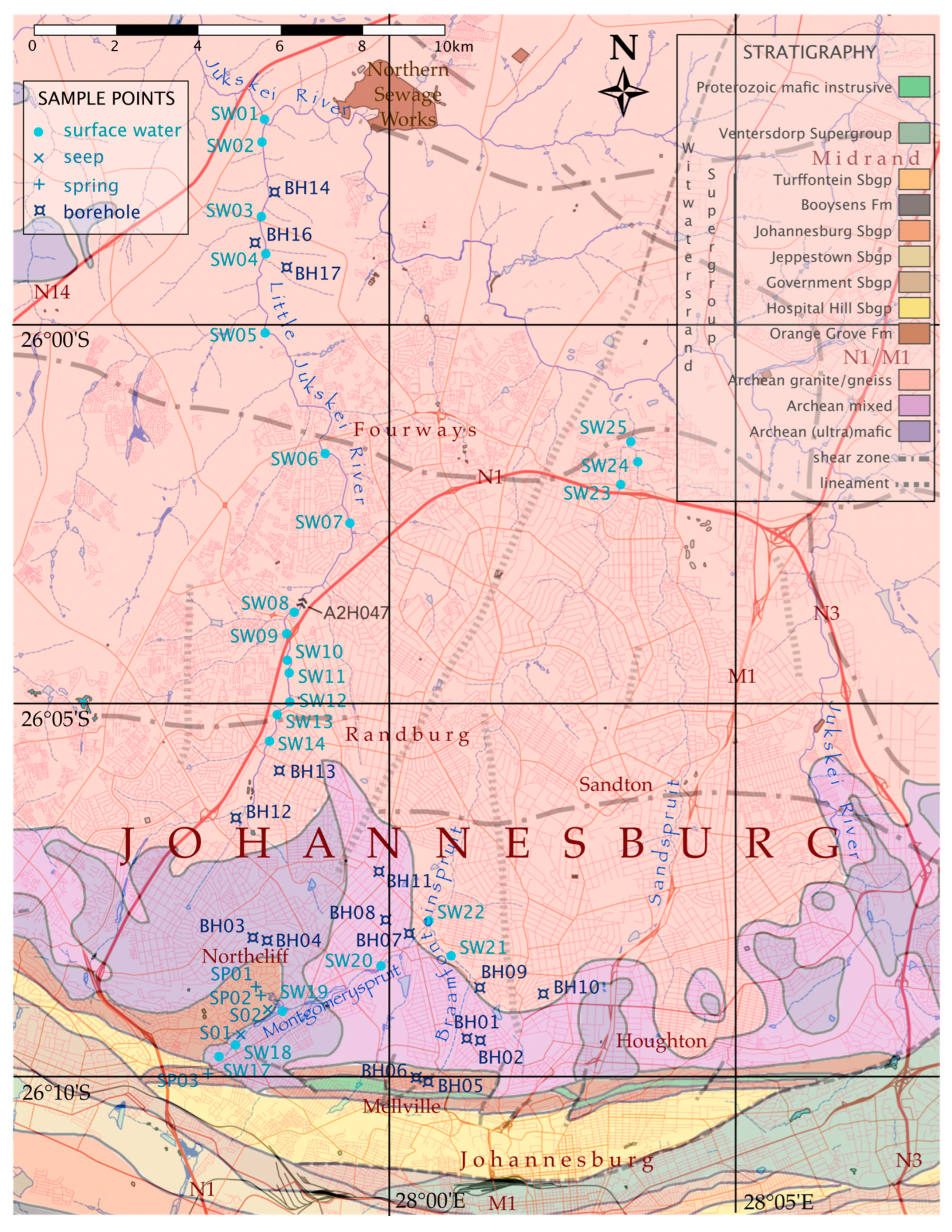
2.1. Location
2.2. Geology
2.3. Climate and Hydrology
2.4. Hydrogeology
3. Materials and Methods
3.1. Sampling
3.2. Measuring Radon and Field Parameters
3.3. Stable Isotopes
3.4. FINIFLUX Model
4. Results and Discussion
4.1. Charcterization of Groundwater and Surface Water
4.1.1. Groundwater
4.1.2. Surfacewater
4.2. Radon as a Tracer for Groundwater Input
4.3. Seasonal Trends and Baseflow Indicators
4.4. Isotope Patterns and Recharge Dynamics
4.5. Structural and Geologic Controls
4.6. Implications for Urban Hydrology and Water Management
5. Conclusions
Author Contributions
Funding
Data Availability Statement
Conflicts of Interest
Abbreviations
| BFI | baseflow index |
| CFCs | chlorofluorocarbons |
| EC | electrical conductivity |
| GWL | groundwater line |
| JRC | Jukskei River Catchment |
| LEL | local evaporation line |
| SMOW | Standard Mean Ocean Water |
| SWL | surface water line |
References
- Charters, F.J.; Cochrane, T.A.; O’Sullivan, A.D. The influence of urban surface type and characteristics on runoff water quality. Sci. Total Environ. 2021, 755, 142470. [Google Scholar] [CrossRef] [PubMed]
- Barnes, M.L.; Welty, C.; Miller, A.J. Impacts of development pattern on urban groundwater flow regime. Water Resour. Res. 2018, 54, 5198–5212. [Google Scholar] [CrossRef]
- O’Driscoll, M.; Clinton, S.; Jefferson, A.; Manda, A.; McMillan, S. Urbanization effects on watershed hydrology and in-stream processes in the southern United States. Water 2010, 2, 605–648. [Google Scholar] [CrossRef]
- Kuhlemann, L.M.; Tetzlaff, D.; Soulsby, C. Urban water systems under climate stress: An isotopic perspective from Berlin, Germany. Hydrol. Process. 2020, 34, 3758–3776. [Google Scholar] [CrossRef]
- Fleckenstein, J.H.; Krause, S.; Hannah, D.M.; Boano, F. Groundwater-surface water interactions: New methods and models to improve understanding of processes and dynamics. Adv. Water Resour. 2010, 33, 1291–1295. [Google Scholar] [CrossRef]
- Boulton, A.J.; Datry, T.; Kasahara, T.; Mutz, M.; Stanford, J. Ecology and management of the hyporheic zone: Stream-groundwater interactions of running waters and their floodplains. J. N. Am. Benthol. Soc. 2010, 29, 26–40. [Google Scholar] [CrossRef]
- Leibowitz, S.; Comeleo, R.; Wigington, P., Jr.; Weaver, C.; Morefield, P.; Sproles, E.; Ebersole, J. Hydrologic landscape classification evaluates streamflow vulnerability to climate change in Oregon, USA. Hydrol. Earth Syst. Sci. 2014, 18, 3367–3392. [Google Scholar] [CrossRef]
- Kuhlemann, L.M.; Tetzlaff, D.; Soulsby, C. Spatio-temporal variations in stable isotopes in per-urban catchments: A preliminary assessment of potential and challenges in assessing streamflow sources. J. Hydrol. 2021, 600, 126685. [Google Scholar] [CrossRef]
- Marx, C.; Tetzlaff, D.; Hinkelmann, R.; Soulsby, C. Isotope hydrology and water sources in a heavily urbanized stream. Hydrol. Process. 2021, 35, e14377. [Google Scholar] [CrossRef]
- Schubert, M.; Siebert, C.; Knoeller, K.; Roediger, R.; Schmidt, A.; Gilfedder, B. Investigating groundwater discharge into a major river under low flow conditions based on a radon mass balance supported by tritium data. Water 2020, 12, 2838. [Google Scholar] [CrossRef]
- Gilfedder, B.S.; Frei, S.; Hoffman, H.; Cartwright, I. Groundwater discharge to wetlands driven by storm and flood events: Quantification using continuous radon-222 and electrical conductivity measurements and dynamic mass-balance modelling. Geochim. Cosmochim. Acta 2015, 165, 161–177. [Google Scholar] [CrossRef]
- Cook, P.G.; Wood, C.; White, T.; Simmons, C.T.; Fass, T.; Brunner, P. Groundwater inflow to a shallow, poorly-mixed wetland estimated from a mass balance of radon. J. Hydrol. 2008, 354, 213–226. [Google Scholar] [CrossRef]
- Burnett, W.C.; Dulaiova, H. Estimating the dynamics of groundwater input into the coastal zone via continuous radon-222 measurements. J. Environ. Radioact. 2003, 69, 21–35. [Google Scholar] [CrossRef]
- Strydom, T.; Nel, J.M.; Nel, M.; Petersen, R.M.; Ramjukadh, C.L. The use of Radon (Rn222) isotopes to detect groundwater discharge in streams draining Table Mountain Group (TMG) aquifers. Water SA 2021, 47, 194–199. [Google Scholar] [CrossRef]
- Jasechko, S. Global Isotope Hydrogeology-Review. Rev. Geophys. 2019, 57, 835–965. [Google Scholar] [CrossRef]
- Soulsby, C.; Birkel, C.; Geris, J.; Tetzlaff, D. Spatial aggregation of time-variant stream water ages in urbanizing catchments. Hydrol. Process. 2015, 29, 3038–3050. [Google Scholar] [CrossRef]
- Rodriguez, F.; Delliou, A.L.L.; Andrieu, H.; Gironas, J. Groundwater contribution to sewer network baseflow in an urban catchment-case study of Pin Sec catchment, Nantes, France. Water 2020, 12, 689. [Google Scholar] [CrossRef]
- Le Maitre, D.C.; Colvin, C. Assessment of the contribution of groundwater discharges to rivers using monthly flow statistics and flow seasonality. Water SA 2008, 34, 549–564. [Google Scholar] [CrossRef]
- Yi, P.; Luo, H.; Chen, L.; Yu, Z.; Jin, H.; Chen, X.; Wan, C.; Aldahan, A.; Zheng, M.; Hu, Q. Evaluation of groundwater discharge into surface water by using radon-222 and the source area of the Yellow River, Qinghai, Tibet Plateau. J. Environ. Radioact. 2018, 192, 257–266. [Google Scholar] [CrossRef] [PubMed]
- Bezuidenhout, J. Estimating indoor radon concentrations based on the uranium content of geological units in South Africa. J. Environ. Radioact. 2021, 234, 106647. [Google Scholar] [CrossRef]
- Yang, J.; Yu, Z.; Yi, P.; Frape, S.K.; Gong, M.; Zhang, Y. Evaluation of surface water and groundwater interactions in the upstream Kui River and Yunlong Lake, Xuzhou, China. J. Hydrol. 2020, 583, 124549. [Google Scholar] [CrossRef]
- Lamontagne, S.; Kirby, J.; Johnston, C. Groundwater-surface water connectivity in a chain of ponds semiarid river. Hydrol. Process. 2021, 35, e14129. [Google Scholar] [CrossRef]
- Cartwright, I.; Gilfedder, B. Mapping and quantifying groundwater inflows to Deep Creek (Marybyrnong catchment, SE Australia) using 222Rn: Implications for protecting groundwater dependant ecosystems. Appl. Geochem. 2015, 52, 118–129. [Google Scholar] [CrossRef]
- Diamond, R.E. Stable Isotope Hydrology; The Groundwater Project: Guelph, ON, Canada, 2022. [Google Scholar]
- Clark, I.D.; Fritz, P. Environmental Isotopes in Hydrogeology; CRC Press: Boca Raton, FL, USA, 2013. [Google Scholar]
- Poujol, M.; Anhaeusser, C. The Johanneburg Dome, South Africa: New single zircon U-Pb isotopic evidence for early Archaean granite-greenstone development within the central Kaapvaal Craton. Precambrian Res. 2001, 108, 139–157. [Google Scholar] [CrossRef]
- Anhaeusser, C. Palaeo- Meso- and Neoarchaean granite-greenstone basement geology and related rocks of the central and western Kaapvaal Craton, South Africa. In The Archaean Geology of the Kaapvaal Craton, Southern Africa, Regional Geology Reviews; Springer: Berlin/Heidelberg, Germany, 2019; Volume 1, pp. 55–81. [Google Scholar]
- Prevec, S.A.; Anhaeusser, C.R.; Poujol, M. Evidence for Archaean lamprophyre from the Kaapvaal Craton, South Africa. S. Afr. J. Sci. 2004, 100, 549–555. [Google Scholar]
- McCarthy, T. The Story of Earth and Life: A Southern African Perspective on a 4.6 Billion Year Journey; Penguin Random House: Midrand, South Africa, 2013. [Google Scholar]
- Eriksson, P.G.; Altermann, W.; Hartzer, F.J. The Geology of South Africa; Number 10; Geological Society of South Africa and Council for Geoscience: Pretoria, South Africa, 2006; Chapter: The Transvaal Supergroup and its precursors; pp. 237–260. [Google Scholar]
- CSAG Climate Systems Analysis Group. 2024. Available online: https://cip.csag.uct.ac.za/ (accessed on 4 February 2024).
- DWS Department of Water and Sanitation. 2023. Available online: https://www.dws.gov.za/hydrology/Verified/HyDataSets.aspx?Station=A2H047 (accessed on 12 August 2023).
- Barnard, H. An Explanation of the 1:500,000 General Hydrogeological Map: Johannesburg 2526; Department of Water Affairs & Forestry: Pretoria, South Africa, 2000. [Google Scholar]
- Leketa, K.; Abiye, T.; Zondi, S.; Butler, M. Assessing groundwater recharge in crystalline and karstic aquifers of the Upper Crocodile River basin, Johannesburg, South Africa. Groundw. Sustain. Dev. 2019, 8, 31–40. [Google Scholar] [CrossRef]
- Durridge. RAD7 H2O Radon in Water Accessory; Owner’s manual; Durridge Inc.: Billerica, MA, USA, 2018. [Google Scholar]
- Frei, S.; Gilfedder, B.S. FINIFLUX: An implicit finite element model for quantification of groundwater fluxes and hyporheic exchange in streams and rivers using radon. Water Resour. Res. 2015, 51, 6776–6786. [Google Scholar] [CrossRef]
- Doherty, J.; Hunt, R.J.; Tonkin, M.J. Approached to Highly Parameterized Inversion: A Guide to Using PEST for Model Parameter and Predictive Uncertainty Analysis; Scientific Investigations Report 5211; USGS: Reston, VA, USA, 2010. [Google Scholar]
- Pittroff, M.; Frei, S.; Gilfedder, B. Quantifying nitrate and oxygen reduction rates in the hyporheic zone using 222Rn to upscale biogeochemical turnover in rivers. Water Resour. Res. 2017, 53, 563–579. [Google Scholar] [CrossRef]
- Cook, P.G.; Herczeg, A.L. (Eds.) Environmental Tracers in Subsurface Flow; Springer Science and Business Media: New York, NY, USA, 2012. [Google Scholar]
- Kiliari, T.; Tsiaili, A.; Pashalidis, I. Lithological and seasonal variations in radon concentrations 534in Cypriot groundwaters. J. Radioanal. Nucl. Chem. 2010, 284, 553–556. [Google Scholar] [CrossRef]
- Tsunomori, R.; Shimodate, T.; Ide, T.; Tanaka, H. Radon concentration distributions in shallow and deep groundwater around the Tachikawa fault zone. J. Environ. Radioact. 2017, 172, 106–112. [Google Scholar] [CrossRef]
- Przylibski, T.A.; Mamont-Ciesla, K.; Kusyk, M.; Dorda, J.; Kozlowska, B. Radon concentrations in groundwaters of the Polish part of the Sudety Mountains (SW Poland). J. Environ. Radioact. 2004, 75, 193–209. [Google Scholar] [CrossRef]
- Hoorzook, K.B.; Pieterse, A.; Heine, L.; Barnard, T.G.; van Rensberg, N.J. Soul of the Jukskei River: The extent of bacterial contamination in the Jukskei River in Gauteng Province, South Africa. Int. J. Environ. Res. Public Health 2021, 18, 8537. [Google Scholar] [CrossRef]
- West, A.G.; February, E.C.; Bowen, G.J. Spatial analysis of hydrogen and oxygen stable isotopes (“isoscapes”) in groundwater and tap water across South Africa. J. Geochem. Explor. 2014, 145, 213–222. [Google Scholar] [CrossRef]
- Leketa, K.; Abiye, T.; Butler, M. Characterisation of groundwater recharge conditions and flow mechanisms in bedrock aquifers of the Johannesburg area, South Africa. Environ. Earth Sci. 2018, 77, 727. [Google Scholar] [CrossRef]
- Terzer, S.; Wassenaar, L.I.; Araguas-Araguas, L.J.; Aggarwal, P.K. Global isoscapes for δ18O and δ2H in precipitation: Improved prediction using regionalized climatic regression models. Hydrol. Earth Syst. Sci. 2013, 17, 4713–4728. [Google Scholar] [CrossRef]
- Jaunat, J.; Huneau, F.; Dupuy, A.; Celle-Jeanton, H.; Vergnaud-Ayraud, V.; Aquilina, L.; Labasque, R.; Coustumer, P.L. Hydrochemical data and groundwater dating to infer differential flowpaths through weathered profiles of a fractured aquifer. Appl. Geochem. 2012, 27, 2053–2067. [Google Scholar] [CrossRef]
- Dhakate, R.; Singh, V. Identification of water-bearing fractured zones using electrical conductivity logging in granitic terrain, Andhra Pradesh, India. Curr. Sci. 2008, 95, 1060–1066. [Google Scholar]
- Cook, P.G. A Guide to Regional Groundwater Flow in Fractured Rock Aquifers; CSIRO Land and Water: Glen Osmond, South Australia, 2003. [Google Scholar]
- McCallum, J.L.; Cook, P.G.; Berhane, D.; Rumpf, C.; McMahon, G.A. Quantifying groundwater flows to streams using differential flow gaugings and water chemistry. J. Hydrol. 2012, 416, 118–132. [Google Scholar] [CrossRef]
- Leketa, K.; Abiye, T. Using environmental tracers to characterize groundwater flow mechanisms in the fractured crystalline and karst aquifers in Upper Crocodile River basin, Johannesburg, South Africa. Hydrology 2021, 8, 50. [Google Scholar] [CrossRef]
- Ogunkoya, O.; Adejuwon, J.; Jeje, L. Runoff response to basin parameters in southwestern Nigeria. J. Hydrol. 1984, 72, 67–84. [Google Scholar] [CrossRef]
- Vogel, J.; van Urk, H. Isotopic composition of groundwater in semi-arid regions of southern Africa. J. Hydrol. 1975, 25, 23–36. [Google Scholar] [CrossRef]
- Diamond, R.E.; Harris, C. Stable isotope constraints on hydrostratigraphy and aquifer connectivity in the Table Mountain Group. S. Afr. J. Geol. 2019, 122, 317–330. [Google Scholar] [CrossRef]
- Carlier, C.; Wirth, S.B.; Cochand, F.; Hunkeler, D.; Brunner, P. Geology controls streamflow dynamics. J. Hydrol. 2018, 566, 756–769. [Google Scholar] [CrossRef]
- Abdou, M.M.; Vandervaere, J.P.; Descroix, L.; Moussa, I.B. Comparative hydrodynamic study of granitic and sedimentary catchments in Western Niger. Hydrol. Sci. J. 2021, 66, 1541–1551. [Google Scholar] [CrossRef]
- Smakhtin, V.U. Low flow hydrology: A review. J. Hydrol. 2001, 240, 147–186. [Google Scholar] [CrossRef]
- Mayer, T.D.; Naman, S.W. Streamflow response to climate as influenced by geology and elevation. J. Am. Water Resour. Assoc. 2011, 47, 724–738. [Google Scholar] [CrossRef]


| Parameter | Description | Units | Comments |
|---|---|---|---|
| streamflow rate | m3·d−1 | measured | |
| groundwater inflow | m3·d−1 | calculated | |
| stream length | m | measured | |
| stream width | m | measured | |
| stream depth | m | measured | |
| stream radon concentration | Bq·m−3 | measured | |
| groundwater radon concentration | Bq·m−3 | measured | |
| gas exchange coefficient | m2·d−1 | known constant | |
| first-order decay constant | d−1 | known constant | |
| hyporheic kinetic production | Bq·m−3·d−1 | calculated | |
| hyporheic kinetic decay | Bq·m−3·d−1 | calculated |
| Sample | Latitude | Longitude | Depth Estimate | Date | δ2H | δ18O | d-Excess | T | pH | EC | Rn Mean | Rn SD |
|---|---|---|---|---|---|---|---|---|---|---|---|---|
| °S | °E | m bgl | ‰ | ‰ | ‰ | °C | μS·cm−1 | Bq·m−3 | ±Bq·m−3 | |||
| BH001 | 26.1629 | 28.0254 | 20 | 21 March | −15.9 | −2.93 | 7.54 | 14.3 | 7.41 | 717 | 14,009 | 4160 |
| BH002 | 26.1638 | 28.0247 | 20 | 21 March | −20.0 | −3.75 | 10.0 | 14.4 | 7.26 | 889 | 6840 | 1470 |
| BH003 | 26.1452 | 27.9757 | 30 | 21 March | −16.8 | −3.04 | 7.52 | 14.7 | 7.40 | 154 | 2940 | 670 |
| BH004 | 26.1442 | 27.9783 | 25 | 21 March | −18.4 | −3.68 | 11.04 | 14.7 | 7.21 | 147 | 1330 | 439 |
| BH005 | 26.1731 | 28.0082 | 10 | 21 March | −19.9 | −4.04 | 12.42 | 17.4 | 7.33 | 321 | 18,006 | 3230 |
| BH006 | 26.1734 | 28.0075 | 15 | 21 March | −7.4 | −1.53 | 4.84 | 17.6 | 7.01 | 536 | 78,009 | 3350 |
| BH007 | 26.1371 | 27.9981 | 10 | 21 March | −12.7 | −3.21 | 12.98 | 16.1 | 7.36 | 154 | 58,007 | 4720 |
| BH008 | 26.1362 | 27.9979 | 21 March | −13.4 | −2.92 | 9.96 | 16.2 | 7.28 | 83 | 52,008 | 4140 | |
| BH009 | 26.1523 | 28.0241 | 20 | 21 March | −12.6 | −2.74 | 9.32 | 15.3 | 7.12 | 221 | 26,006 | 3210 |
| BH010 | 26.1539 | 28.0404 | 20 | 21 March | −18.5 | −3.78 | 11.74 | 15.5 | 7.23 | 265 | 42,006 | 3430 |
| BH011 | 26.1265 | 27.9968 | 120 | 21 March | −16.9 | −3.57 | 11.66 | 16 | 7.55 | 527 | 196,000 | 9000 |
| BH012 | 26.1127 | 27.9616 | 50 | 21 July | −14.5 | −3.44 | 13.02 | 13.1 | 7.13 | 261 | 21,009 | 2320 |
| BH013 | 26.1019 | 27.9678 | 40 | 21 July | −25.4 | −4.78 | 12.84 | 19 | 7.41 | 145 | 174,000 | 10,000 |
| BH014 | 25.9721 | 27.9666 | 20 | 21 July | −19.2 | −3.71 | 10.48 | 14.1 | 7.43 | 761 | 2290 | 870 |
| BH016 | 25.9834 | 27.9613 | 25 | 21 July | −22.8 | −4.46 | 12.88 | 20.2 | 7.37 | 525 | 57,005 | 3330 |
| BH017 | 25.9953 | 27.9769 | 21 July | −28.0 | −5.27 | 14.16 | 21 | 7.56 | 154 | 70,000 | 1360 | |
| S01 | 26.16452 | 27.96506 | 21 August | −18.89 | −3.77 | 11.27 | 16.6 | - | 370 | 910 | 377 | |
| S02 | 26.15933 | 27.97414 | 21 August | −15.72 | −3.23 | 10.12 | 20.3 | - | 175 | 7322 | 1046 | |
| SP001 | 26.1552 | 27.9700 | 21 March | −13.8 | −2.98 | 10.04 | 25.2 | 7.50 | 141 | 17,003 | 2130 | |
| 21 May | −16.8 | −3.46 | 10.88 | 17.2 | 7.11 | 154 | 29,005 | 3620 | ||||
| 21 July | −17.3 | −3.62 | 11.66 | 18 | 7.63 | 150 | 28,000 | 2170 | ||||
| 21 September | −14.6 | −2.98 | 9.24 | 21.4 | 7.28 | 162 | 14,370 | 1060 | ||||
| SP002 | 26.1555 | 27.9702 | 21 March | − | − | - | 19.8 | 6.62 | 158 | 30,007 | 5130 | |
| 21 May | − | − | - | 25.6 | 7.47 | 144 | 38,004 | 4430 | ||||
| 21 July | − | − | - | 17.2 | 7.61 | 130 | 41,003 | 3910 | ||||
| 21 September | − | − | - | 18.3 | 7.30 | 131 | 33,000 | 4520 | ||||
| SP003 | 26.1697 | 27.96 | 21 March | −16.4 | −4.32 | 18.16 | 22.3 | 7.41 | 103 | 3970 | 694 | |
| 21 July | −19.6 | −3.81 | 10.88 | 26.1 | 7.40 | 121 | 2940 | 503 | ||||
| 21 September | −20.4 | −3.86 | 10.48 | 17.4 | 7.57 | 144 | 4370 | 560 | ||||
| means | −17.78 | −3.61 | 11.01 | 18.22 | 7.37 | 274 | 36,875 | 2960 |
| Sample | Date | δ2H | δ18O | d-Excess | EC | Rn Mean | Rn SD |
|---|---|---|---|---|---|---|---|
| ‰ | ‰ | ‰ | μS·cm−1 | Bq·m−3 | ±Bq·m−3 | ||
| SW01 | 21 March | −16.6 | −3.12 | 8.36 | 473 | 1678 | 179 |
| 21 July | − | − | − | 421 | 1567 | 208 | |
| 21 September | −15.8 | −2.72 | 5.96 | 444 | 1080 | 117 | |
| SW02 | 21 March | −15.2 | −2.71 | 6.48 | 468 | 1006 | 240 |
| 21 July | − | − | 422 | 1127 | 354 | ||
| 21 September | −14.0 | −2.16 | 3.28 | 451 | 988 | 321 | |
| SW03 | 21 March | −15.8 | −3.02 | 8.36 | 460 | 414 | 198 |
| 21 July | − | − | 566 | 403 | 191 | ||
| 21 September | −16.2 | −3.39 | 10.92 | 421 | 376 | 84 | |
| SW04 | 21 March | −18.1 | −3.06 | 6.38 | 506 | 512 | 265 |
| 21 July | − | − | − | 412 | 441 | 234 | |
| 21 September | −14.6 | −2.48 | 5.24 | 447 | 562 | 129 | |
| SW05 | 21 September | −15.9 | −2.66 | 5.38 | 422 | 403 | 111 |
| SW06 | 21 September | −15.0 | −2.38 | 4.04 | 472 | 1419 | 450 |
| SW07 | 21 September | −14.4 | −2.42 | 4.96 | 359 | 367 | 189 |
| SW08 | 21 March | − | − | − | 353 | 642 | 234 |
| 21 July | −16.6 | −2.93 | 6.84 | 362 | 705 | 198 | |
| 21 September | − | − | 374 | 638 | 202 | ||
| SW09 | 21 March | −14.8 | −2.96 | 8.88 | 334 | 1870 | 750 |
| 21 July | − | − | − | 421 | 2001 | 767 | |
| SW10 | 21 March | −15.3 | −2.98 | 8.54 | 373 | 2080 | 483 |
| 21 July | − | − | − | 365 | 2012 | 501 | |
| 21 September | −14.1 | −2.89 | 9.02 | 291 | 2001 | 557 | |
| SW11 | 21 March | −15.1 | −3.07 | 9.46 | 365 | 1040 | 417 |
| 21 July | − | − | 476 | 876 | 306 | ||
| 21 September | −14.2 | −2.91 | 9.08 | 321 | 921 | 261 | |
| SW12 | 21 March | −15.6 | −2.95 | 8.0 | 363 | 1940 | 436 |
| 21 July | − | − | 374 | 1234 | 675 | ||
| 21 September | −13.8 | −3.03 | 10.44 | 403 | 1255 | 370 | |
| SW13 | 21 March | −15.5 | −2.96 | 8.18 | 364 | 1250 | 481 |
| 21 July | − | − | − | 372 | 1116 | 527 | |
| SW14 | 21 March | −15.5 | −2.97 | 8.26 | 366 | 830 | 279 |
| 21 July | − | − | − | 402 | 710 | 321 | |
| SW15 | 21 March | −15.8 | −3.25 | 10.2 | 543 | 1250 | 970 |
| SW16 | 21 March | −14.1 | −3.0 | 9.9 | 385 | 1040 | 796 |
| SW17 | 21 October | − | − | − | 180 | 2530 | 830 |
| SW18 | 21 July | −14.9 | −3.15 | 10.3 | 394 | 796 | 224 |
| SW19 | 21 March | −15.4 | −2.97 | 8.36 | 491 | 877 | 142 |
| SW20 | 20 August | −10.9 | −2.28 | 7.31 | 480 | 1422 | 460 |
| SW21 | 21 July | −14.1 | −2.76 | 7.98 | 410 | 1240 | 425 |
| SW22 | 21 July | −14.6 | −2.77 | 7.56 | 437 | 1180 | 532 |
| SW23 | 21 July | −15.5 | −3.09 | 9.22 | 556 | 1660 | 679 |
| SW24 | 21 March | − | − | − | 409 | 416 | 208 |
| SW25 | 21 March | −13.4 | −2.49 | 6.52 | 392 | 479 | 115 |
| means | −15.03 | −2.85 | 7.78 | 411 | 1099 | 373 |
Disclaimer/Publisher’s Note: The statements, opinions and data contained in all publications are solely those of the individual author(s) and contributor(s) and not of MDPI and/or the editor(s). MDPI and/or the editor(s) disclaim responsibility for any injury to people or property resulting from any ideas, methods, instructions or products referred to in the content. |
© 2025 by the authors. Licensee MDPI, Basel, Switzerland. This article is an open access article distributed under the terms and conditions of the Creative Commons Attribution (CC BY) license (https://creativecommons.org/licenses/by/4.0/).
Share and Cite
Diphofe, K.; Diamond, R.; Kotze, F. Quantifying Baseflow with Radon, H and O Isotopes and Field Parameters in the Urbanized Catchment of the Little Jukskei River, Johannesburg. Hydrology 2025, 12, 203. https://doi.org/10.3390/hydrology12080203
Diphofe K, Diamond R, Kotze F. Quantifying Baseflow with Radon, H and O Isotopes and Field Parameters in the Urbanized Catchment of the Little Jukskei River, Johannesburg. Hydrology. 2025; 12(8):203. https://doi.org/10.3390/hydrology12080203
Chicago/Turabian StyleDiphofe, Khutjo, Roger Diamond, and Francois Kotze. 2025. "Quantifying Baseflow with Radon, H and O Isotopes and Field Parameters in the Urbanized Catchment of the Little Jukskei River, Johannesburg" Hydrology 12, no. 8: 203. https://doi.org/10.3390/hydrology12080203
APA StyleDiphofe, K., Diamond, R., & Kotze, F. (2025). Quantifying Baseflow with Radon, H and O Isotopes and Field Parameters in the Urbanized Catchment of the Little Jukskei River, Johannesburg. Hydrology, 12(8), 203. https://doi.org/10.3390/hydrology12080203