Abstract
This study assesses the accuracy of flood extent predictions in five U.S. watersheds. We generated flood maps for four return periods using various digital elevation models (DEMs)—FABDEM, SRTM, ALOS, and USGS 3DEP—and two versions of the GEOGLOWS River Forecast System (RFS) hydrography. These comparisons are notable because they build on operational global hydrology models so subsequent work can develop global modeled flood products. Models were made using the Automated Rating Curve (ARC) and Curve2Flood tools. Accuracy was measured against USGS reference maps using the F-statistic. Our results show that flood map accuracy generally increased with higher return periods. The most consistent and reliable improvements in accuracy occurred when both the DEM and hydrography datasets were upgraded to higher-resolution sources. While DEM improvements generally had a greater impact, hydrography refinements were more important for lower return periods when flood extents were the smallest. Generally, DEM resolution improved accuracy metrics more as the return period increased and hydrography and bare earth DEMs mattered more as the return period decreased. There was a 38.9% increase in the mean F-statistic between the two principal pairings of interest (FABDEM-RFS2 and SRTM 30 m DEM-RFS1). FABDEM’s bare-earth representation combined with RFS2 sometimes outperformed higher-resolution non-bare-earth DEMs, suggesting that there remains a need for site-specific investigation. Using ARC and Curve2Flood with FABDEM and RFS2 is a suitable baseline combination for general flood extent application.
1. Introduction
1.1. Large Scale Flood Mapping Efforts
Flood maps provide valuable information for a variety of fields including emergency management, insurance rates, urban planning, agriculture, and ecology. Efforts to create large-scale flood maps include programs such as FEMA’s Risk Mapping, Assessment, and Planning (Risk MAP) program, which develops flood risk products and updates the regulatory Flood Insurance Rate Maps (FIRMs) used for the National Flood Insurance Program (NFIP). Tools such as the United States Geological Survey (USGS) Flood Inundation Mapper [1] offer interactive flood extent visualizations based on real-time and historical streamflow data. In Europe, initiatives such as the Copernicus Emergency Management Service (CEMS) provide detailed flood maps [2]. There are ongoing efforts to support less developed regions with similar information, leveraging global models and satellite technology to enhance flood risk assessment and resilience by utilizing datasets that are globally accessible and well-suited for flood risk assessment [2,3].
When flood mapping tools are combined with streamflow outputs from hydrologic models, flood extents can be generated over large areas. The flood maps are usually generated using lower complexity hydraulic modeling methods such as Height Above Nearest Drainage (HAND) [4], AutoRoute [5,6,7], Automated Rating Curve (ARC) [8], and Flood Inundation Surface Topology Tool (FIST) [9] for flood map production [10]. A primary justification for these methods is the general absence of high-fidelity information required as inputs to 1D and 2D models along with the impractical costs and time required to build, calibrate, and compute those simulations routinely. One concrete example of a group taking this approach is the United States’ National Water Center under NOAA which uses HAND to generate flood inundation maps alongside their hydrology model, the National Water Model. Another example is the U.S. Military who implements the Streamflow Prediction Tool with hydrological data and maps based on shuttle elevation derivatives at multiple scales (HydroSHEDS) to predict discharge, and AutoRoute and FloodSpreader to simulate flood inundations [7].
The skill of these flood map modeling systems is constrained by the skill of the hydrological predictions and the quality of hydraulic datasets, particularly digital elevation models (DEMs) and river channel hydrography [4,11,12,13]. Hydrodynamic modeling studies emphasize that while large-scale flood models can simulate flood inundation extents, uncertainties remain due to errors in terrain representation and river bathymetry [14,15]. Additionally, the accuracy of DEM-derived hydrography is a limiting factor in flood modeling, as many existing datasets lack the resolution needed for precise river channel delineation [16,17]. Addressing these limitations requires higher-resolution DEMs and hydrography data to enhance flood modeling accuracy.
1.2. Global Elevation Data Sources
To maximize potential model skill in any hydraulic model, but especially the methods used for large scale efforts, high-quality elevation data is the foundation. Ideally, the hydrography, hydrology model, and flood maps are made on a shared set of inputs, including the DEM [18]. Misaligned DEM and stream hydrography can result in spatial mismatches between channel locations according to the DEM and stream hydrography, which can cause many kinds of errors [19]. This limitation has been documented in evaluations of low-complexity flood models applied at continental scales [5,15].
In this study, we evaluate flood inundation maps using four DEM sources, namely, the Shuttle Radar Topography Satellite Mission (SRTM) 30 and 90 m DEMs [20], the Forest and Buildings removed Copernicus DEM (FABDEM), ALOS DEM, and the USGS 3DEP 10 m DEM. SRTM is the most widely used global DEM for hydrology [21,22,23,24]. More recently, the TanDEM-X mission’s propriety 12 m DEM and several public derivatives such as the WorldDEM and the Copernicus DEM have demonstrated significant improvement [15,21]. While these datasets serve as the foundation for large-scale hydrologic applications, ongoing research aims to evaluate their effectiveness in improving flood model accuracy [25,26]. In addition, the ALOS DEM is a global 12 m DEM option which is higher spatial resolution than the FABDEM but is not a bare earth dataset. Since the subject areas for flood maps presented in Section 2.1 are all in the United States, we will also consider 12 m DEMs from the USGS as another point of comparison for the highest resolution widely available DEM options but note that this is not globally available.
Table 1 summarizes several properties of the DEM datasets used as sources for the hydrography and elevations used for evaluating flood maps. Notably, the TanDEM-X DEM source is used to derive both the RFS2 hydrography and the FABDEM.

Table 1.
Comparison of TanDEM-X and SRTM satellite missions.
The SRTM DEM was produced by NASA in February 2000 using interferometric synthetic aperture radar (InSAR) to create two DEMs at 90 and 30 m resolutions and was the best available global dataset at the time [20]. SRTM captured the elevation of vegetation and structures rather than bare-earth terrain, introducing significant errors for hydrologic modeling. Data quality concerns have been documented including bias, striping, speckling, and voids where radar signals were obstructed [15,30]. These limitations impact hydrologic applications by affecting river network delineation and flow path accuracy [26]. Despite these issues, SRTM remains widely used and is the foundation of several processed hydrography datasets, including HydroSHEDS and MERIT Hydro [15,21].
The TanDEM-X mission, completed in 2016, produced a DEM with a 12 m spatial resolution and a 2 m vertical accuracy [27]. The mission used radar interferometers on two TerraSAR-X radar satellites [27]. The raw TanDEM-X DEM remains private but was used to create the Copernicus 30 m global digital elevation model (COPDEM30) which is publicly available [31]. COPDEM30 offers enhanced terrain representation with reduced pixel noise and high elevation consistency [27,32]. COPDEM30 forms the basis for further refined DEM products such as Forest and Buildings removed Copernicus DEM (FABDEM). FABDEM is a 30 m resolution global digital elevation model designed to enhance hydrologic applications by removing the elevation of vegetation and built structures using machine learning [26]. FABDEM enhances river network alignment and improves floodplain delineation in large-scale flood modeling studies by providing a more hydrologically consistent terrain representation [33]. Compared to traditional DEMs like SRTM, which retain vegetation-induced elevation biases, FABDEM provides a more accurate representation of the bare-earth surface, making it particularly valuable for flood mapping and hydrologic simulations where precise flow path modeling is crucial [26]. The ALOS DEM, derived from the PALSAR sensor onboard the ALOS mission, has been applied in numerous global studies [28,34,35,36]. The ALOS DEM is radiometric terrain corrected to remove geometric and radiometric distortions [28,36,37]. It is publicly accessible and has a spatial resolution of 12 m. The USGS 1/3 arc second DEM is derived from a variety of data sources (primarily LIDAR), is continuously updated as part of the USGS’ 3D Elevation Program. and is an authoritative, high-resolution dataset for the United States [29].
1.3. Global Hydrography Data Sources
While hydrography datasets may describe many surface water and ocean features, for this research we are concerned only with the stream centerline vector datasets used by hydrology and hydraulic models. Several options exist for hydrography datasets for global-scale flood modeling, each with different resolutions and conditioning [21,25]. We use the Group on Earth Observations’ Global Water Sustainability (GEOGLOWS) River Forecasting System (RFS) datasets from their original and more recent second versions [38,39,40].
RFS Version 1 (RFS1) is derived from the same elevation source as HydroSHEDS, a global hydrography dataset developed from SRTM [21,38]. This makes the stream feature placement typically identical to HydroSHEDS but developed with the purpose of building a version suitable for a global hydrology model. These streams are consistent with SRTM elevations, so flood maps generated with SRTM and RFSV1 hydrography are coming from the same source elevation representation.
RFS Version 2 (RFS2) is derived from the TanDEM-X Hydro (TDX-Hydro) dataset, with several edits including dropping small watersheds and correcting errors found in the TDX-Hydro dataset [21,25]. TDX-Hydro, derived from TanDEM-X, improves on HydroSHEDS by using a finer-resolution DEM and more advanced hydrologic conditioning techniques [25]. Comparisons indicate that TDX-Hydro provides more precise river alignments and stream connectivity, reducing errors commonly found in previous global hydrography datasets [25]. Flood maps made using FABDEM, derived from TanDEM-X, and RFS2 hydrography, derived from TanDEM-X are generated using datasets all sharing the same source elevation representation. Figure 1 is a map showing a representative comparison of the difference in RFS1 and RFS2 hydrographys. Two pertinent features are that the RFS2’s higher resolution source DEM allows the stream centerlines to more smoothly follow the river paths in the basemap and traces streams in more locations.
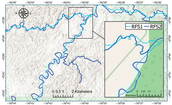
Figure 1.
Representative comparison of hydrography RFS2 and RFS1 in the Amazon region of Ecuador.
1.4. Research Objective
The primary combinations of datasets being evaluated in this paper are the SRTM and FABDEM elevation datasets along with hydrography derived from them used in RFSV1 and RFSV2. For greater rigor, we also evaluate flood maps made using each hydrography option and the ALOS DEM and USGS DEM. The reason for using the RFS hydrography products instead of their better-known but similar products, HydroSHEDS and TDX-Hydro, is that RFS provides retrospective and forecast river discharge simulations on these versions of the stream representation. Evaluating flood map skill based on these combinations is conducted with the intent to design a system for global flood mapping expanding on the RFS. This manuscript is an initial assessment of methods and datasets for building an addition to the RFS system.
We conduct eight sets of trials using each possible combination of the four DEM datasets and the two hydrography datasets. We use the Automated Rating Curve (ARC) and Curve2Flood methods [41,42] to generate flood inundation maps. We evaluate the model-generated inundation extents against reference maps from USGS sources at five sites, developed from high-resolution in situ observations [1]. At each of the five sites, flood maps are simulated to match four different flow levels which approximate 2-, 10-, 50-, and 100-year return period level events. We evaluate the combinations of maps made to evaluate the effect of hydrography and DEM data selection on the accuracy of flood maps [16,25,26].
2. Methods
2.1. Study Areas and Flood Scenarios
We used maps from the USGS as our reference or “ground truth” flood maps. They are based on recorded flood events, high-resolution LIDAR, stream gauge data, surveyed high water marks, and the Hydrologic Engineering Center’s River Analysis System (HEC-RAS) 1D-or-2D models to produce the flood extents [1,43,44,45,46,47]. Summary details of each site and references to additional explanations of the reference maps are given in Table 2. The study areas, shown in Figure 2, include the Suncook River in New Hampshire, the North Fork Kentucky River in Kentucky, Nimishillen Creek in Ohio, the Flathead River in Montana, and the South Platte River at Fort Morgan in Colorado. These locations cover a range of hydrological and geographic conditions.
Table 2.
Site description and details.
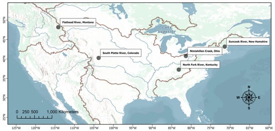
Figure 2.
Study site locations.
We selected four discharge scenarios for each study site to evaluate flood extents under varying flow conditions. These categories were chosen to approximate the 2-year, 10-year, 50-year, and 100-year flood events, respectively, as defined by FEMA. While exact FEMA flow values were not always modeled directly in the reference flood inundation maps, we used the closest available USGS-modeled discharges in the map to model flood inundation using ARC. When no USGS-modeled flow matched the FEMA benchmark, we used log-log interpolation between known return period discharges—typically between the FEMA-reported 2-year, 10-year, 50-year, 100-year, and 500-year events—to estimate the return period associated with each USGS-modeled flow [48,49].
2.2. ARC and Curve2Flood Method Overview
We used ARC in this study which is a raster-based flood inundation model based on the core functionality of AutoRoute while offering improved accessibility and adaptability. AutoRoute was developed by the U.S. Army Corps of Engineers Coastal and Hydraulics Laboratory to assess route vulnerability for military vehicles during flood events [6] using automated cross-section extraction and DEM-derived stream masks [6,7]. The utility of ARC for flood inundation modeling has been evaluated through comparisons with USGS flood maps, using the ARC-Curve2Flood workflow in various test cases [41]. Because the model does not incorporate detailed two-dimensional hydraulic calculations, it requires significantly fewer computational resources than higher fidelity 2D hydrodynamic models such as HEC-RAS 2D, thus supporting modeling larger regions and high resolution datasets [6,7]. This lower complexity means that for complex hydrodynamic systems like coasts, braided streams, culverts, low topographic relief, and bridges, ARC-Curve2Flood will perform poorly. However, these limitations have been shown to be less impactful as the modeled discharge and depth increase [50].
Over time, AutoRoute was adapted for large-scale flood modeling applications, particularly in data-sparse regions where traditional hydraulic models are computationally prohibitive [6,7]. It allows for rapid dataset switching with minimal preprocessing, making it well-suited for comparing different DEM and hydrography resolutions [5]. AutoRoute balances computational efficiency and accuracy by reducing processing requirements while maintaining suitable performance for global applications [7].
Curve2Flood is a postprocessing script that visualizes the hydraulic calculations and produces the final flood extent map based on ARC outputs. These simulations used ARC hydraulic parameters, which drove Curve2Flood for inundation map visualization. Low, median, and high flow events were simulated across several test cases and compared with USGS flood maps. The F-statistic [51] and error bias [10] were used to assess the agreement between the map sets. The findings indicated that the F-statistic values for ARC-Curve2Flood were similar in magnitude to those found for AutoRoute-FloodSpreader simulations [7], suggesting a comparable level of accuracy. However, the error bias indicated that ARC-Curve2Flood results generally had a higher tendency to over-predict flooding compared to AutoRoute-FloodSpreader results [7], particularly in the Muskingum River and Susquehanna River test cases.
AutoRoute has been compared with other flood inundation models, namely HAND (Height Above Nearest Drainage) and HEC-RAS 2D [5]. While AutoRoute and HAND use Manning’s equation, their approach to inundation mapping differs significantly. HAND employs a lateral approach, relying on precomputed stage-discharge relationships rather than direct hydraulic calculations at each cross-section [5]. Evaluations showed that AutoRoute generally provides more accurate flood extents than HAND, particularly in areas characterized by moderate to high terrain relief [7]. AutoRoute tends to outperform HAND in capturing variations in flood extent. Conversely, HAND generally provides more reliable depth estimations in deeper channels, where AutoRoute’s reliance on DEM-based cross-section sampling can introduce uncertainties [5]. AutoRoute is less accurate when compared to the more complex HEC-RAS 2D model, which accounts for backwater effects and the influence of levees [5].
The ARC model follows a modeling process similar to AutoRoute, which follows the structured workflow shown in Figure 3. ARC ingests hydrography, land cover raster, DEM, and streamflow datasets. ARC extracts river cross-sections from the DEM at each stream cell and estimates water depth, top-width, and velocity using Manning’s equation (Equation (1)) where Q is the discharge, A is the flow area, R is the hydraulic radius, S is the slope, and n is Manning’s roughness coefficient derived from land cover data [48]. Previous flood modeling experiments using ARC and Curve2Flood showed general insensitivity in Manning’s n values [52]. The final output is generated using a postprocessing tool that translates the stage-discharge relationships into spatial flood extents. This structured process enables ARC to produce flood maps across various datasets rapidly.
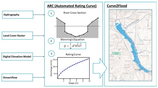
Figure 3.
ARC workflow from data ingestion, through calculation, and results visualization.
2.3. Flood Map Production
We generated flood maps using an exhaustive pairing of the FABDEM and the SRTM DEMs with the RFS1 and RFS2 hydrography datasets. Comparisons between FABDEM-RFS1 and FABDEM-RFS2, and between SRTM-RFS1 and SRTM-RFS2, assess the impact of hydrography refinement while keeping the elevation model constant. Similarly, comparisons between FABDEM-RFS1 and SRTM-RFS1, and between FABDEM-RFS2 and SRTM-RFS2, isolate the effect of DEM resolution while maintaining a consistent hydrography dataset. This approach enables us to evaluate the individual contributions of DEM and hydrography refinements to the accuracy of the flood inundation model.
We assessed flood inundation map accuracy primarily using the fitness statistic (F) as the key evaluation metric, as it provides a comprehensive measure of agreement between modeled and reference flood extents. We used a two-by-two contingency matrix [53] to classify each pixel into four categories: true positive (TP), where the model correctly predicts a flooded pixel; true negative (TN), where the model correctly predicts a non-flooded pixel; false positive (FP), where the model predicts flooding but the reference map does not; and false negative (FN), where the model predicts a dry pixel but the reference map indicates flooding.
Previous AutoRoute studies demonstrated that the F-statistic provides a reliable performance measure, making it particularly useful for large-scale flood modeling applications [7]. We used the median instead of the mean to summarize F-statistic which mitigates the influence of outliers [54]. While overall trends were consistent across study locations, variability in F-statistic was sufficient to warrant using the median, which is less sensitive to extreme values than the mean [54]. Using the median more accurately represents agreement between modeled and observed flood extents, while reducing metrics from highly skewed cases. The F-statistic, also known as the Critical Success Index (CSI) [54], ranges from 0 to 1, with one being the most favorable (Equation (2)).
We computed additional performance metrics, including Proportion Correct (PC), Bias (B), Hit Rate (H), and Kappa (K) [54], for reference. In this paper, we primarily discuss the F-statistic, however the other metrics described below can be found in the supplemental dataset for each study area, DEM-hydrography pairing, and flow condition.
Proportion Correct (PC) scores range from 0 to 1, with a score of 1 being the best (Equation (3)). Although PC is a widely adopted metric, it cannot differentiate between False Positives (FP) and False Negatives (FN), as both are treated equally [55].
Bias (B) is a positive value, ideally equal to 1. It is not an accuracy measure [54], but it shows if the scene is generally overestimated (B > 1) or underestimated (B < 1) (Equation (4)). It is important to note that B does not measure model performance. Instead, it indicates how often the model overestimates versus underestimates. So, a B value of 1 does not mean the model is highly accurate; it just means it makes about the same number of over- and underestimations [55].
Hit Rate (H) ranges from 0 to 1, with 1 being the best (Equation (5)). H measures how many flooded pixels on the reference maps are correctly predicted. It is also called the Probability of Detection (POD), true-positive fraction, or sensitivity [54].
Kappa Value (K) can be negative, indicating that the prediction is worse than a random guess (Equation (6)) [56]. The best value for K is 1.
3. Results
3.1. General Trends from All Simulations
We evaluated simulations from all combinations of DEM, hydrography, and return period for each site. The full table of values is available in the data availability statement. We found several trends. First, we found that, in general, F-statistic increased as the simulated return period increased regardless of which DEM and hydrography combination used. This trend applied when aggregating F-statistic across all sites as well as for any individual site; however, some sites had less significant total increase than others. One relevant outlier is at the lowest return period simulated, 2-year, where the FABDEM option typically had a larger F-statistic than either the ALOS or USGS DEMs. This trend may be attributable to the impact of the bare-earth representation combined with hydrography derived from the same underlying digital elevation, TanDEM-X. A bar chart illustrating this observation is given in Figure 4.
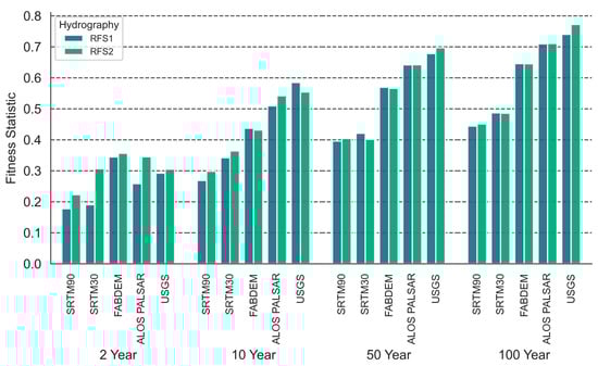
Figure 4.
Average simulated fitness statistic across all sites for each return period, DEM, and hydrography.
Table 3 contains the calculated values averaged across all locations for Proportion Correct, Bias, Hit Rate, and Kappa. These values for proportion correct are very close to 1, the best value, because this metric considers true negatives and weighs them as important as true positives. However, the overall trend matches the other metrics. The values for bias indicate that the reason the lower return periods do worse is because the model is overpredicting. As the return period increases, the model’s bias approaches 1. The values for Hit Rate are highest for the higher resolution DEMs and for RFS2, and are very close to 1 with the USGS DEM for all return periods except return period 2, where both the ALOS DEM and FABEM perform mildly better. The Kappa value is mathematically related to the F-Statistic and so demonstrates the same trends.
Table 3.
Proportion Correct, Bias, Hit Rate, and Kappa averaged across all locations for every return period, DEM, and Hydrography combination.
Figure 5 presents the effect of switching from RFS1 to RFS2 (referred to as the “hydrography improvement”) or switching from the SRTM 30 m DEM to the FABDEM (referred to as the “DEM improvement”), within each return period and across all test locations. To isolate the influence of each component, we computed the F-statistic from two comparisons: (1) using the FABDEM and SRTM 30 m DEM as the DEM base while switching hydrography from RFS1 to RFS2, and (2) using RFS1 and RFS2 as the hydrography base while switching DEMs from the SRTM 30 m DEM to the FABDEM. The left side shows the increase in the F-statistic due to hydrography upgrades, while the right side shows the corresponding effect of DEM upgrades.
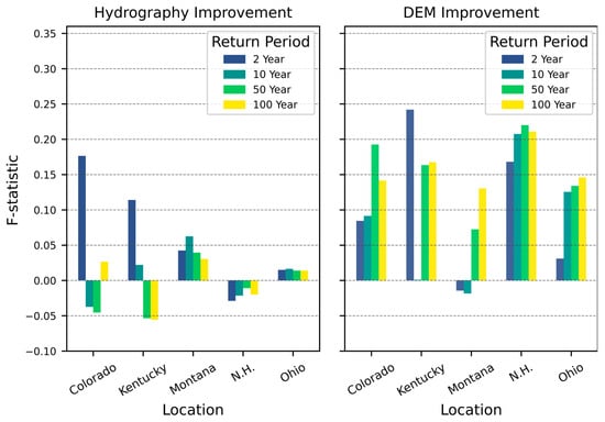
Figure 5.
F-statistic change for the improved Hydrography (left) or DEM (right) datasets.
While most return periods and locations had mixed benefits from improved hydrography (with a mean increase in F-statistic of 0.015), most scenarios show more significant gains from DEM improvements (with a mean increase in F-statistic of 0.125). This trend is also seen in Figure 4, where the highest resolutions DEMs (like the ALOS and USGS DEMs) perform better than FABDEM, which performs better than the SRTM 30 m DEM, with the SRTM 90 m DEM performing the worst. This suggests that it is the combination of both the higher accuracy hydrography and (most importantly) the higher-resolution DEMs that produces flood extents with consistently higher F-statistic. Figure 6 confirms that implication by showing that all sites at all return periods exhibited increased F-statistic when using the FABDEM-RFS2 combination relative to the SRTM-RFS1 combination. Notably, for some locations the hydrography improvement produces large gains at low return periods (this is seen also in Figure 4).
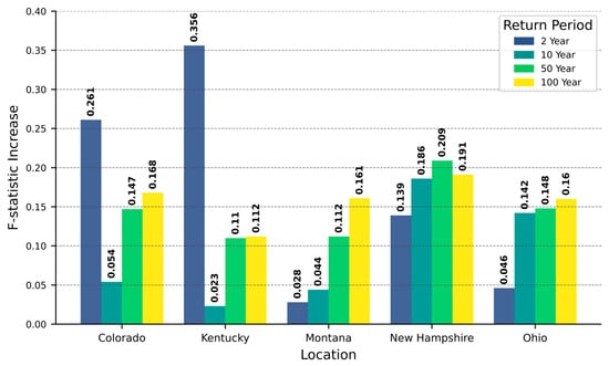
Figure 6.
Difference in F-statistic between FABDEM-RFS2 and SRTM-RFS1 for 5 sites and 4 return periods.
The FABDEM-RFS2 pairing consistently produced a higher F-statistic than the SRTM-RFS1 combination across all five study sites and all four return periods. Specifically, between FABDEM-RFS2 and SRTM-RFS1, there was a mean increase in the F-statistic of 0.139, or a 38.9% increase. From both Figure 4 and Figure 6, flood map agreement improves the most when both the DEM and hydrography datasets matched each other and were from higher resolution satellite missions.
Figure 7 shows a representative example of the flood extents from the Colorado location for a 100-year return period. The improved accuracy, as reflected in a higher F-statistic, likely results from a combination of improved vertical accuracy, lower spatial representation error for the hydrography, and bare-earth processing that eliminated issues associated with vegetation.
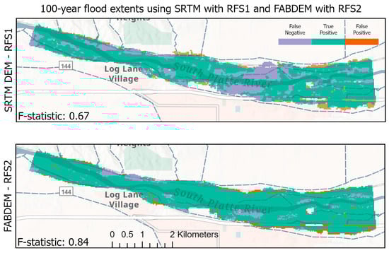
Figure 7.
The 100-year flood extents in Fort Morgan, Colorado, using SRTM with RFS1 (top) and FABDEM with RFS2 (bottom).
These results are consistent with previous studies using AutoRoute and noting limitations in low-flow conditions. Those studies showed flood extent estimates tend to be overestimated, particularly in flatter terrain, due to simplified bathymetry representation and the lack of multidimensional hydraulic modeling [7].
3.2. Extending the Evaluation to Additional DEM Elevations for Flood Mapping
Recognizing that DEM accuracy has a larger impact on improving flood inundation modeling, we added the USGS and ALOS high-resolution DEMs to our comparisons with both RFS1 and RFS2 hydrography. We compared the F-statistic obtained from different DEM data sources to both hydrography data sources.
Figure 8 shows a comparison of the median F-statistic across return periods for the selected locations for the RFS1 and RFS2 datasets, respectively. The higher-resolution elevation data consistently yielded higher F-statistic values without respect to the underlying hydrography. While both the hydrography and elevation data affect the flood extents, as previously noted, elevation data exerted stronger influence in the F-statistic. The sharp drop in the F-statistic for the SRTM-90 DEM is expected because of its relatively low resolution. However, even when using a hydrography not defined from the same elevation source, as was the case for the RFS2 and FABDEM combination in the previous analysis, improvement was seen using the highest resolution and presumably more accurate USGS and ALOS DEMs.
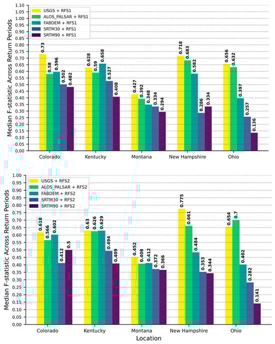
Figure 8.
Median F-statistic of all return periods presented for each dataset and each location.
While the general trend shows that the USGS DEM is superior, followed by ALOS, then FABDEM, SRTM-30 and SRTM-90, there are some locations where the FABDEM outperformed the higher-resolution DEMs. Figure 9 shows the F-statistic aggregated across both hydrographys for all four return periods at the Kentucky location. The performance at this location is superior to the USGS and ALOS DEMs for three of the four return periods. We hypothesize that the impact of the bare earth DEM could make a larger difference in some locations, though further studies at more locations would be required to verify this result.
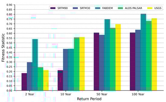
Figure 9.
Fitness statistic for each return period and DEM averaged over hydrography for the Kentucky site.
3.3. Evaluation of Selected Flood Extent Maps
Besides the F-statistic, a visual comparison of maps is valuable to better understand performance. Considering the many different combinations of hydrography and DEM, it is impossible to share all the results generated in this manuscript. We share here some selected examples mapped for the Colorado location, whereas results for other locations are included in the data availability section.
Figure 10 shows flood extents at the Colorado location for the lowest return period modeled. At lower return periods, there is not widespread flooding as water is just beginning to overtop the banks. The improved F-statistic with RFS2 and FABDEM reflects the importance of accurate placement of the hydrography within the DEM is particularly important for lower return periods. In the top image, RFS1′s stream centerlines are not well aligned with the channel in the DEM as indicated by the false positive results shown in areas that are disconnected from the actual river. In the bottom image, RFS2′s centerlines, being from the same underlying elevation data, agree more with FABDEM, leading to less over and underprediction in comparison.
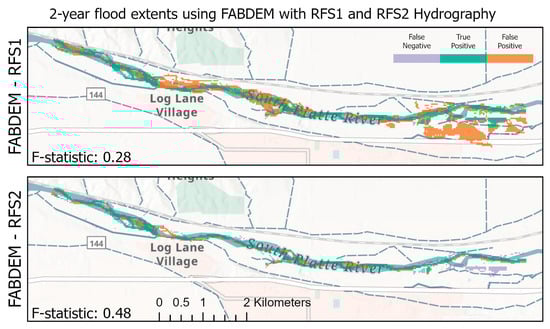
Figure 10.
Two-year flood extents in Fort Morgan, Colorado, using FABDEM with RFS1 (top) and RFS2 (bottom).
Figure 11 shows the Colorado site for the 100-year return period flood. Here we see little difference in the overall flood map comparisons, with no discontinuities of the flood zones as can be seen with RFS1 in the lower return periods, even though the hydrography is not well aligned in some places. However, there does seem to be some under-prediction of flooding with RFS1 as seen on the left side of the maps even though the overall F-statistic is not significantly different.
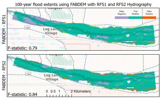
Figure 11.
100-year flood extents in Fort Morgan, Colorado, using FABDEM with RFS1 (top) and RFS2 (bottom).
Figure 12 also shows the Colorado site for the 100-year return period where this time, instead of comparing the RFS1 and RFS2 hydrography, we examine the improvement based on the DEM resolution. Consistent with previous results, the more accurate DEM produces the higher F-statistic, though the USGS and FABDEM perform similarly (F-statistic of 0.87 and 0.84, respectively) and both significantly better than the coarser SRTM (F-statistic 0.68).
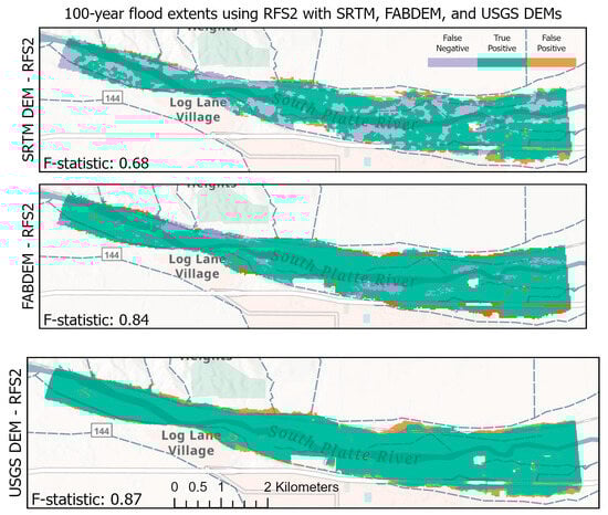
Figure 12.
The 100-year flood extents in Fort Morgan, Colorado, using SRTM (top), FABDEM (middle), and USGS (bottom) DEMs with RFS2.
4. Conclusions
This manuscript presents an experiment building flood maps using the ARC and Curve2Flood methods at five sites with combinations of four DEM inputs, two hydrography inputs, and four return period level flows. We observed that the F-statistic generally increased as the simulated return period increased, regardless of the DEM and hydrography combination used. This trend was observed across all sites and individual sites, though the magnitude of increase varied. Our focus was on the change in F-statistic between the FABDEM-RFS2 pairing and the SRTM 30 m-RFS1 pairing. The transition from the lower-resolution SRTM 30 m-RFS1 combination to the higher-resolution FABDEM-RFS2 pairing consistently yielded more accurate flood inundation maps, as indicated by a steady increase in F-statistic across all five study locations and all return periods. Overall, there was a 38.9% increase in mean F-statistic between the two pairings. Using FABDEM with RFS1 or SRTM with RFS2 did not yield the same accuracy gains, underscoring the importance of using terrain and stream network data derived from same source and at the highest resolution and fidelity possible.
Improvements to the DEM had a more pronounced impact on the F-statistic than hydrography alone, shown by an increase in the F-statistic value of 0.125. When examining the median of F-statistic across the four return periods within each dataset combination, results were generally higher for combinations that included the higher resolution RFS2 hydrography. The USGS 3DEP 10 m DEM generally showed superior performance, followed by ALOS, FABDEM, SRTM-30 m, and SRTM-90 m. However, the FABDEM sometimes outperformed higher-resolution non-bare-earth DEMs (like ALOS or USGS 3DEP) at the lowest return period (2-year flow). This suggests that the bare-earth representation of FABDEM, combined with RFS2 hydrography derived from the same underlying TanDEM-X elevation data, is particularly important for lower flows but also higher flows at some locations. Switching from RFS1 to RFS2 played a more significant role in accuracy improvement at lower return periods, particularly the 2-year return period. These results indicate that small errors in stream alignment and floodplain connectivity have a larger impact in flood inundation extent at low flows.
The presented research is regionally focused in the United States owing to the availability of reconstructed maps for specific events coming from the USGS. Future work should include more total sites and ideally many sites representative of different kinds of physical characteristics. Those maps should be accompanied by analysis of site properties which may better characterize trends in performance at untested locations. Because of the limited number of sites, we recommend caution expecting the specific magnitudes of increase or decrease in performance at other sites. These findings are generally supportive of additional work using these datasets and methods.
The ARC and Curve2Flood tools combined with the globally available FABDEM and RFS2 can be recommended as generally the best option for accurate flood maps at lower flows, while ALOS or better-resolution, but perhaps not global coverage, DEMs with RFS2 are usually best at higher flows. Future flood inundation mapping initiatives should prioritize staying current with the release of global DEMs and advanced processing methods that further improve vertical accuracy, spatial resolution, and bare-earth representation to enhance the accuracy of flood maps.
Author Contributions
Conceptualization, T.J.M., R.C.H. and R.C.H.; Data curation, R.C.H. and E.J.N.; Formal analysis, T.J.M., L.R.R. and J.L.G.; Funding acquisition, R.C.H. and E.J.N.; Investigation, T.J.M., M.L.F., L.R.R. and J.L.G.; Methodology, T.J.M., M.L.F., R.C.H., E.J.N. and G.P.W.; Project administration, R.C.H., E.J.N., G.P.W. and N.L.J.; Resources, R.C.H. and E.J.N.; Software, T.J.M., M.L.F., L.R.R., R.C.H. and E.J.N.; Supervision, R.C.H., E.J.N. and G.P.W.; Validation, T.J.M., M.L.F., L.R.R., R.C.H. and E.J.N.; Visualization, T.J.M., M.L.F., L.R.R., J.L.G., R.C.H. and E.J.N.; Writing—original draft, T.J.M., M.L.F., L.R.R., R.C.H., E.J.N. and E.J.N.; Writing—review and editing, T.J.M., M.L.F., L.R.R., J.L.G., R.C.H., E.J.N., G.P.W. and N.L.J. All authors have read and agreed to the published version of the manuscript.
Funding
This research was funded by NASA grant numbers SERVIR 80NSSC23K0180 and 80NSSC22K0927. Part of this research was supported through the Cooperative Institute for Research to Operations in Hydrology (CIROH) with funding under award NA22NWS4320003 from the NOAA Cooperative Institute Program. The statements, findings, conclusions, and recommendations are those of the author(s) and do not necessarily reflect the opinions of NOAA. The funders had no role in the design of the study; in the collection, analyses, or interpretation of data; in the writing of the manuscript; or in the decision to publish the results.
Data Availability Statement
All the modeled flood maps are available as a zip file via Zenodo at https://doi.org/10.5281/zenodo.15588365.
Acknowledgments
We express gratitude to the USGS and GEOGLOWS programs whose work produced the datasets that are the foundation of experimentation in the paper. We also thank Follum Hydrologic Solutions for making ARC and Curve2Flood publicly available and for their assistance using these tools to make many flood maps.
Conflicts of Interest
Authors Michael L. Follum and Joseph L. Gutenson were employed by the company Follum Hydrologic Solutions, LLC. The remaining authors declare that the research was conducted in the absence of any commercial or financial relationships that could be construed as a potential conflict of interest.
References
- Flood Inundation Mapper. Available online: https://fim.wim.usgs.gov/fim/ (accessed on 11 April 2025).
- Salamon, P.; Mctlormick, N.; Reimer, C.; Clarke, T.; Bauer-Marschallinger, B.; Wagner, W.; Martinis, S.; Chow, C.; Bohnke, C.; Matgen, P.; et al. The New, Systematic Global Flood Monitoring Product of the Copernicus Emergency Management Service. In Proceedings of the 2021 IEEE International Geoscience and Remote Sensing Symposium IGARSS, Brussels, Belgium, 11 July 2021; IEEE: New York City, NY, USA, 2021; pp. 1053–1056. [Google Scholar]
- Dottori, F.; Salamon, P.; Bianchi, A.; Alfieri, L.; Hirpa, F.A.; Feyen, L. Development and Evaluation of a Framework for Global Flood Hazard Mapping. Adv. Water Resour. 2016, 94, 87–102. [Google Scholar] [CrossRef]
- Nobre, A.D.; Cuartas, L.A.; Momo, M.R.; Severo, D.L.; Pinheiro, A.; Nobre, C.A. HAND Contour: A New Proxy Predictor of Inundation Extent. Hydrol. Process. 2016, 30, 320–333. [Google Scholar] [CrossRef]
- Afshari, S.; Tavakoly, A.A.; Rajib, M.A.; Zheng, X.; Follum, M.L.; Omranian, E.; Fekete, B.M. Comparison of New Generation Low-Complexity Flood Inundation Mapping Tools with a Hydrodynamic Model. J. Hydrol. 2018, 556, 539–556. [Google Scholar] [CrossRef]
- Follum, M.L. AutoRoute Rapid Flood Inundation Model; ERDC/CHL CHETN; US Army Engineer Research and Development Center, Coastal and Hydraulics Laboratory: Vicksburg, MS, USA, 2013. [Google Scholar]
- Follum, M.L.; Tavakoly, A.A.; Niemann, J.D.; Snow, A.D. AutoRAPID: A Model for Prompt Streamflow Estimation and Flood Inundation Mapping over Regional to Continental Extents. J. Am. Water Resour. Assoc. 2017, 53, 280–299. [Google Scholar] [CrossRef]
- Follum, M.L. Automated-Rating-Curve. Available online: https://github.com/MikeFHS/automated-rating-curve/wiki/Home (accessed on 23 May 2025).
- Dobbs, K. Flood Inundation Surface Topology (FIST) Modeling and Applications. Available online: https://bluewaters.ncsa.illinois.edu/science-teams@page=detail&psn=bazt (accessed on 14 April 2025).
- Wing, O.E.J.; Quinn, N.; Bates, P.D.; Neal, J.C.; Smith, A.M.; Sampson, C.C.; Coxon, G.; Yamazaki, D.; Sutanudjaja, E.H.; Alfieri, L. Toward Global Stochastic River Flood Modeling. Water Resour. Res. 2020, 56, e2020WR027692. [Google Scholar] [CrossRef]
- Ward, E. Global Sensitivity Analysis of Terrain Effects in Geolocation Systems. IEEE Trans. Aerosp. Electron. Syst. 2015, 51, 2039–2046. [Google Scholar] [CrossRef]
- Olsen, N.R.; Tavakoly, A.A.; McCormack, K.A.; Levin, H.K. Effect of User Decision and Environmental Factors on Computationally Derived River Networks. J. Geophys. Res. Earth Surf. 2023, 128, e2022JF006873. [Google Scholar] [CrossRef]
- Tarboton, D.G.; Bras, R.L.; Rodriguez-Iturbe, I. On the Extraction of Channel Networks from Digital Elevation Data. Hydrol. Process. 1991, 5, 81–100. [Google Scholar] [CrossRef]
- Schumann, G.J.-P.; Bates, P.D.; Neal, J.C.; Andreadis, K.M. Chapter 2—Measuring and Mapping Flood Processes. In Hydro-Meteorological Hazards, Risks and Disasters; Shroder, J.F., Paron, P., Baldassarre, G.D., Eds.; Elsevier: Boston, MA, USA, 2015; pp. 35–64. ISBN 978-0-12-394846-5. [Google Scholar]
- Yamazaki, D.; Ikeshima, D.; Tawatari, R.; Yamaguchi, T.; O’Loughlin, F.; Neal, J.C.; Sampson, C.C.; Kanae, S.; Bates, P.D. A High-accuracy Map of Global Terrain Elevations. Geophys. Res. Lett. 2017, 44, 5844–5853. [Google Scholar] [CrossRef]
- Aristizabal, F.; Chegini, T.; Petrochenkov, G.; Salas, F.; Judge, J. Effects of High-Quality Elevation Data and Explanatory Variables on the Accuracy of Flood Inundation Mapping via Height Above Nearest Drainage. Hydrol. Earth Syst. Sci. 2024, 28, 1287–1315. [Google Scholar] [CrossRef]
- Xu, K.; Fang, J.; Fang, Y.; Sun, Q.; Wu, C.; Liu, M. The Importance of Digital Elevation Model Selection in Flood Simulation and a Proposed Method to Reduce DEM Errors: A Case Study in Shanghai. Int. J. Disaster Risk Sci. 2021, 12, 890–902. [Google Scholar] [CrossRef]
- Sampson, C.C.; Smith, A.M.; Bates, P.D.; Neal, J.C.; Trigg, M.A. Perspectives on Open Access High Resolution Digital Elevation Models to Produce Global Flood Hazard Layers. Front. Earth Sci. 2016, 3, 85. [Google Scholar] [CrossRef]
- Johnson, J.M.; Munasinghe, D.; Eyelade, D.; Cohen, S. An Integrated Evaluation of the National Water Model (NWM)–Height Above Nearest Drainage (HAND) Flood Mapping Methodology. Nat. Hazards Earth Syst. Sci. 2019, 19, 2405–2420. [Google Scholar] [CrossRef]
- Farr, T.G.; Rosen, P.A.; Caro, E.; Crippen, R.; Duren, R.; Hensley, S.; Kobrick, M.; Paller, M.; Rodriguez, E.; Roth, L.; et al. The Shuttle Radar Topography Mission. Rev. Geophys. 2007, 45, RG2004. [Google Scholar] [CrossRef]
- Lehner, B.; Verdin, K.; Jarvis, A. New Global Hydrography Derived from Spaceborne Elevation Data. Eos Trans. Am. Geophys. Union 2008, 89, 93–94. [Google Scholar] [CrossRef]
- Lehner, B.; Grill, G. Global River Hydrography and Network Routing: Baseline Data and New Approaches to Study the World’s Large River Systems. Hydrol. Process. 2013, 27, 2171–2186. [Google Scholar] [CrossRef]
- Frasson, R.P.D.M.; Pavelsky, T.M.; Fonstad, M.A.; Durand, M.T.; Allen, G.H.; Schumann, G.; Lion, C.; Beighley, R.E.; Yang, X. Global Relationships Between River Width, Slope, Catchment Area, Meander Wavelength, Sinuosity, and Discharge. Geophys. Res. Lett. 2019, 46, 3252–3262. [Google Scholar] [CrossRef]
- Yan, D.; Wang, K.; Qin, T.; Weng, B.; Wang, H.; Bi, W.; Li, X.; Li, M.; Lv, Z.; Liu, F.; et al. A Data Set of Global River Networks and Corresponding Water Resources Zones Divisions. Sci. Data 2019, 6, 219. [Google Scholar] [CrossRef]
- Carlson, K.A.; Levin, H.K.; Morris, A.L.; Candela, S.G.; Rivera, A.M.M.; Huening, V.G.; Fredericks, J.G. TDX-Hydro: Global High-Resolution Hydrography Derived from TanDEM-X. ESS Open Arch. 2024. [Google Scholar] [CrossRef]
- Hawker, L.; Uhe, P.; Paulo, L.; Sosa, J.; Savage, J.; Sampson, C.; Neal, J. A 30 m Global Map of Elevation with Forests and Buildings Removed. Environ. Res. Lett. 2022, 17, 024016. [Google Scholar] [CrossRef]
- Krieger, G.; Moreira, A.; Fiedler, H.; Hajnsek, I.; Werner, M.; Younis, M.; Zink, M. TanDEM-X: A Satellite Formation for High-Resolution SAR Interferometry. IEEE Trans. Geosci. Remote Sens. 2007, 45, 3317–3341. [Google Scholar] [CrossRef]
- Rosenqvist, A.; Shimada, M.; Ito, N.; Watanabe, M. ALOS PALSAR: A Pathfinder Mission for Global-Scale Monitoring of the Environment. IEEE Trans. Geosci. Remote Sens. 2007, 45, 3307–3316. [Google Scholar] [CrossRef]
- 1/3rd Arc-Second Digital Elevation Models (DEMs)-USGS National Map 3DEP Downloadable Data Collection-ScienceBase-Catalog. Available online: https://www.sciencebase.gov/catalog/item/4f70aa9fe4b058caae3f8de5 (accessed on 9 May 2025).
- Riegler, G.; Hennig, S.D.; Weber, M. WORLDDEM—A Novel Global Foundation Layer. Int. Arch. Photogramm. Remote Sens. Spatial Inf. Sci. 2015, XL-3/W2, 183–187. [Google Scholar] [CrossRef]
- European Space Agency. Airbus Copernicus DEM. Available online: https://doi.org/10.5270/ESA-c5d3d65 (accessed on 30 July 2025).
- Huang, J.; Yang, Y. Vertical Accuracy Assessment of the ASTER, SRTM, GLO-30, and ATLAS in a Forested Environment. Forests 2024, 15, 426. [Google Scholar] [CrossRef]
- Nandam, V.; Patel, P.L. A Framework to Assess Suitability of Global Digital Elevation Models for Hydrodynamic Modelling in Data Scarce Regions. J. Hydrol. 2024, 630, 130654. [Google Scholar] [CrossRef]
- Zandsalimi, Z.; Feizabadi, S.; Yazdi, J.; Salehi Neyshabouri, S.A.A. Evaluating the Impact of Digital Elevation Models on Urban Flood Modeling: A Comprehensive Analysis of Flood Inundation, Hazard Mapping, and Damage Estimation. Water Resour. Manag. 2024, 38, 4243–4268. [Google Scholar] [CrossRef]
- Pandya, D.; Rana, V.K.; Suryanarayana, T.M.V. Inter-Comparison and Assessment of Digital Elevation Models for Hydrological Applications in the Upper Mahi River Basin. Appl. Geomat. 2024, 16, 191–214. [Google Scholar] [CrossRef]
- Ferreira, Z.; Cabral, P. Vertical Accuracy Assessment of ALOS PALSAR, GMTED2010, SRTM and Topodata Digital Elevation Models. In Proceedings of the 7th International Conference on Geographical Information Systems Theory, Applications and Management—GISTAM, Online, 23–25 April 2021; SciTePress: Setubal, Portugal, 2021; pp. 116–124. [Google Scholar]
- Shimada, M.; Itoh, T.; Motooka, T.; Watanabe, M.; Shiraishi, T.; Thapa, R.; Lucas, R. New Global Forest/Non-Forest Maps from ALOS PALSAR Data (2007–2010). Remote Sens. Environ. 2014, 155, 13–31. [Google Scholar] [CrossRef]
- Ashby, K.R.; Hales, R.C.; Nelson, J.; Ames, D.P.; Williams, G.P. Hydroviewer: A Web Application to Localize Global Hydrologic Forecasts. Open Water J. 2021, 7, 9. [Google Scholar]
- Hales, R.C.; Nelson, E.J.; Souffront, M.; Gutierrez, A.L.; Prudhomme, C.; Kopp, S.; Ames, D.P.; Williams, G.P.; Jones, N.L. Advancing Global Hydrologic Modeling with the GEOGloWS ECMWF Streamflow Service. J. Flood Risk Manag. 2025, 18, e12859. [Google Scholar] [CrossRef]
- Hales, R.C.; Nelson, E.J.; Kopp, S.; Levin, H.K.; Morris, A.L.; Souffront Alcantara, M.A.; Gutiérrez, A.; Magoffin, R.H.; Rosas, L.; Baaniya, Y. The Second Generation Geoglows River Forecast System. SSRN 2025. [Google Scholar] [CrossRef]
- Gutenson, J.L. How Has Curve2Flood Performed Compared to USGS Flood Inundation Maps? Available online: https://github.com/MikeFHS/curve2flood/wiki/How-has-Curve2Flood-performed-compared-to-USGS-flood-inundation-maps%3F (accessed on 28 March 2025).
- MikeFHS MikeFHS/Automated-Rating-Curve. Available online: https://github.com/MikeFHS/automated-rating-curve (accessed on 11 April 2025).
- Boldt, J.A.; Lant, J.G.; Kolarik, N.E. Flood-Inundation Maps for the North Fork Kentucky River at Hazard, Kentucky; U.S. Geological Survey: Reston, VA, USA, 2018. [Google Scholar]
- Flynn, R.H.; Johnston, C.M.; Hayes, L. Flood-Inundation Maps for the Suncook River in Epsom, Pembroke, Allenstown, and Chichester, New Hampshire; U.S. Geological Survey: Reston, VA, USA, 2012. [Google Scholar]
- Kohn, M.S.; Patton, T.T. Flood-Inundation Maps for the South Platte River at Fort Morgan, Colorado, 2018; U.S. Geological Survey: Reston, VA, USA, 2018. [Google Scholar]
- Price, A. Flood-Inundation Maps for the Flathead River from Columbia Falls, Montana to the Holt Stage Road Bridge Near Kalispell, Montana, 2017; U.S. Geological Survey: Reston, VA, USA, 2017. [Google Scholar]
- Whitehead, M. Flood-Inundation Maps for Nimishillen Creek Near North Industry, Ohio, 2019. Available online: https://pubs.usgs.gov/publication/sir20195083 (accessed on 12 April 2025).
- Chow, V.T.; Maidment, D.R.; Mays, L.W. Applied Hydrology; McGraw-Hill Series in Water Resources and Environmental Engineering; McGraw-Hill: New York, NY, USA, 1988; ISBN 0-07-010810-2. [Google Scholar]
- England, J.F.; Cohn, T.A.; Faber, B.A.; Stedinger, J.R.; Thomas, W.O.; Veilleux, A.G.; Kiang, J.E.; Mason, R.R. Guidelines for Determining Flood Flow Frequency-Bulletin 17C. In U.S. Geological Survey Techniques and Methods, Book 4; U.S. Geological Survey: Reston, VA, USA, 2018. [Google Scholar]
- Follum, M.L.; Vera, R.; Tavakoly, A.A.; Gutenson, J.L. Improved Accuracy and Efficiency of Flood Inundation Mapping of Low-, Medium-, and High-Flow Events Using the AutoRoute Model. Nat. Hazards Earth Syst. Sci. 2020, 20, 625–641. [Google Scholar] [CrossRef]
- Bates, P.D.; De Roo, A.P.J. A Simple Raster-Based Model for Flood Inundation Simulation. J. Hydrol. 2000, 236, 54–77. [Google Scholar] [CrossRef]
- Praskievicz, S.; Carter, S.; Dhondia, J.; Follum, M. Flood-Inundation Modeling in an Operational Context: Sensitivity to Topographic Resolution and Manning’s n. J. Hydroinform. 2020, 22, 1338–1350. [Google Scholar] [CrossRef]
- Provost, F.; Kohavi, R. Guest Editors’ Introduction: On Applied Research in Machine Learning. Mach. Learn. 1998, 30, 127–132. [Google Scholar] [CrossRef]
- Wilks, D.S. Statistical Methods in the Atmospheric Sciences; Elsevier: Amsterdam, The Netherlands, 2019; ISBN 978-0-12-815823-4. [Google Scholar]
- Li, Z.; Duque, F.Q.; Grout, T.; Bates, B.; Demir, I. Comparative Analysis of Performance and Mechanisms of Flood Inundation Map Generation Using Height Above Nearest Drainage. Environ. Model. Softw. 2023, 159, 105565. [Google Scholar] [CrossRef]
- Juurlink, D.N.; Detsky, A.S. Kappa Statistic. CMAJ 2005, 173, 16. [Google Scholar] [CrossRef]
Disclaimer/Publisher’s Note: The statements, opinions and data contained in all publications are solely those of the individual author(s) and contributor(s) and not of MDPI and/or the editor(s). MDPI and/or the editor(s) disclaim responsibility for any injury to people or property resulting from any ideas, methods, instructions or products referred to in the content. |
© 2025 by the authors. Licensee MDPI, Basel, Switzerland. This article is an open access article distributed under the terms and conditions of the Creative Commons Attribution (CC BY) license (https://creativecommons.org/licenses/by/4.0/).