Significance of Spring Inflow to Great Salt Lake, Utah, U.S.A.

Abstract

Spring waters (n = 103) from locations surrounding Great Salt Lake (GSL) were mapped, collected, and analyzed to determine their chemical compositions. A ternary Ca-SO₄-alkalinity plot was used to group these waters into compositional types based on the principle of chemical divides. Different spring water types were mixed with Bear, Jordan, and Weber River waters to determine the amount of spring inflow needed to reproduce the chemical composition of GSL. The Pitzer-based computer program EQL/EVP was used to simulate evaporation of spring-river water mixtures. The goal was to find spring-river water mixtures that, when evaporated, reproduced the chemical composition of modern GSL. This approach yielded GSL brine composition from a starting mixture of 12% spring inflow and 88% river water, by volume. The calculated spring inflow–river water mixture contains, on a molar percentage basis, greater than 50% of the B, K, Li, Na, and Cl supplied by springs and greater than 50% of the Ba, Ca, Sr, SO₄, and alkalinity derived from rivers. Understanding GSL spring inflow and brine evolution as lake elevation drops is critical to lake environments, ecosystems, and industrial brine shrimp harvesting and mineral extraction.

1. Introduction

Great Salt Lake (GSL), Utah, is the largest lake in the United States west of the Mississippi River [1] and the eighth largest saline lake in the world (Figure 1) [2]. GSL has an average maximum depth of ~9 m at an assumed lake level of 1280 m above sea level (masl) [3] and an area of approximately 4400 square kilometers in an average year [4]. An earthen railroad causeway built in 1959 has separated GSL into two bays, Gunnison (North Arm) and Gilbert (South Arm), which limits hydrologic mixing between the two arms. Drought and extensive water use for irrigation and human development have recently brought GSL to its lowest levels in recorded history [2,5]. The long standing historic low level of GSL was 1277.7 masl in 1963 [6,7]. Fifty-eight years later, on 23 July 2021, GSL reached a new historic record low level of 1277.5 masl at the U.S. Geological Survey (USGS) Saltair gauge, and by 12 August 2021, the South Arm of GSL reached a level of 1277.4 masl [7]. This record stood until November 2022, when GSL reached a new record low level of 1276.6 masl at the USGS South Arm Causeway gauge [8,9].

The Great Salt Lake is in danger of drying up, which would produce major ecological consequences for wildlife from loss of both open-water and wetland habitats [5,10]. GSL is an important habitat for migratory birds, brine shrimp (Artemia franciscana), brine flies (Ephydra cineria; Ephydra hians), and microbialites that are the keystone building block for the overall ecosystem [11,12]. Waterfowl and other shorebirds rely on GSL wetlands as a migratory resting ground and GSL brine shrimp as a primary food source [5,10]. The drying of GSL impacts the brine shrimp industry because higher salinity levels from lake shrinkage stress brine shrimp habitats [2,5,12]. GSL brines are produced for Mg, K₂SO₄, and KCl [13], but low lake levels make access to brines for processing more difficult [2]. Last, drying of GSL could pose human health problems because exposed lakeshore playas will generate dust particles that could blow clouds containing arsenic, lanthanum, lithium, and zirconium toward Salt Lake City and the Wasatch Mountain front [14,15].

Understanding inflow waters is important for monitoring the future of GSL. Three rivers (Bear River, Weber River, and Jordan River) are estimated to represent ~95% of the total volume of inflow water to GSL [16,17]. Groundwater was estimated to represent 3% of the total volume of inflow to GSL between 1931 and 1976 [18,19]. The remaining 2% is made up of inflow from Davis Creek, Goggin Drain, and Lee Creek, meteoric precipitation, and runoff [16,17]. Surface water inflows were used to determine the evolution of GSL salt loads over the past 35,000 years [20,21]; groundwater and spring inflow was assumed to be 3% or not considered at all [22]. Spring inflow must contribute significantly to the chemical composition of GSL because evaporation of river inflow waters cannot alone produce the correct ionic proportions in the lake brines [17,20]. Recent estimates of groundwater inflow to GSL, using the Darcy flux equation and a seepage velocity method in ArcGIS, are much higher, 10 and 11% of the total volume of inflow, respectively [23]. That groundwater inflow volume represents ~10% of the total solutes derived from inflow waters to GSL [23].

Hydrothermal and continental groundwaters influence brine type evolution in endorheic basins [24,25]. Magmatic-derived solute sources are typically fault controlled or long-distance transported by riverine input or by basinal springs that have diagenetically interacted with basement and sedimentary rocks. Case studies from the Qaidam Basin in China, Salar de Atacama in Chile, and Death Valley and Bristol Dry Lake in the U.S.A., have all exhibited present and past brine evolutions influenced by hydrothermal Ca-Cl inflow waters. Additionally, the chemical composition of inflow waters and their evolution have been inferred from preserved evaporite sequences and associated deposits in closed basins. Chemical analysis of fluid inclusions in halite and evaporite minerals in Searles Lake, U.S.A., have shown that major ion compositions of inflow waters changed by distant hydrothermal activity in the Long Valley caldera region [25]. The inflow waters crossed the CaCO₃ chemical divide and produced alkaline brines, which were essential for the formation of sodium carbonate evaporite minerals in Searles Lake [26].

Here we report the chemical compositions of spring and river waters that flow into GSL, and GSL brines from the North Arm and South Arm. River waters, springs, North Arm and South Arm brines, and previously measured river and spring discharge data were used to construct a mass balance model that produced the chemical composition of modern GSL brines. The mass balance model was then used to assess the relative contributions of spring and river inflow to the GSL solute load.

1.1. Study Area

Great Salt Lake is located in the tectonically active Great Basin, defined by mountain ranges separated by north–south normal faults from sediment-filled basins [27,28]. The last major earthquake (magnitude 5.7 in 2020) occurred along the Wasatch Fault System near GSL (Figure 1) [27,29,30]. Paleozoic and Mesozoic sedimentary and metamorphic rocks are exposed in the Wasatch Mountains and Cenozoic lacustrine and alluvial sediments comprise the GSL valley-fill deposits [27]. Pleistocene igneous activity provides local geothermal sources, in particular, three eroded shield volcanoes, between ~0.44 and ~1.16 Ma in age, located north of GSL (Figure 1; [27,31]). Lake Bonneville, the precursor lake to GSL, occupied an area of ~51,300 km² at its peak in the late Pleistocene [32]. Lake Bonneville was a pluvial lake from ~30,000 years ago to ~13,000 years ago, after which it evolved into a smaller saline lake, more or less the same depth and size as modern GSL [6]. The average level of GSL between 1847 and 2021 was 1280 masl over an area of 2626 km² in the South Arm and 1558.8 km² in the North Arm [16,33,34].

A railroad causeway was built across GSL in 1959 by the Union Pacific Railroad Company, dividing it and limiting flow between two, now separate, brine bodies (Figure 1). The separation of the North and South Arms of GSL reduced freshwater inflow to the North Arm from the South Arm which caused the salinity of the North Arm to increase to 34% and reach saturation with respect to halite during most summer and fall months since 1959 [5,17,21,33,35,36]. The Bear, Weber, and Jordan Rivers all enter the South Arm of GSL. The salinity of the South Arm is, thus, lower than the North Arm, typically varying between 12 and 15% [5,21,33]. This study measured salinity to be 17% in June 2021.

In the 1980s, GSL had annual inflow that was 240 percent above the long-term average [33,37], which caused it to reach a high of 1284 masl on 3 June 1986. At that time, the salinity of the North Arm decreased, and the salt crust dissolved [6,33]. When GSL levels rose, two 4.6 m wide culverts were emplaced along the causeway to improve hydraulic exchange between the South and North Arms, but they rapidly filled with debris. In 1984, an 88.3 m wide breach was opened on the western end of the causeway to allow surface water flow from the South Arm to flood into the North Arm. The culverts were decommissioned from 2012 to 2013 due to structural failure and the western breach has been shallow (<~0.5 m) due to low lake elevations.

In December 2016, a bridge constructed on the railroad causeway created a new opening for water to flow between the North and South Arms. When the bridge opened, the North Arm was at its historic low of ~1276.8 masl [17]. This breach allowed greater hydrologic exchange between the North and South Arms for management purposes, which would decrease the salinity of the North Arm brines and raise North Arm brine elevation [35]. North Arm waters since 2016 have fluctuated seasonally between super- and undersaturated conditions with respect to halite. Significant halite precipitation began in late 2020 [17].

1.2. Previous Work

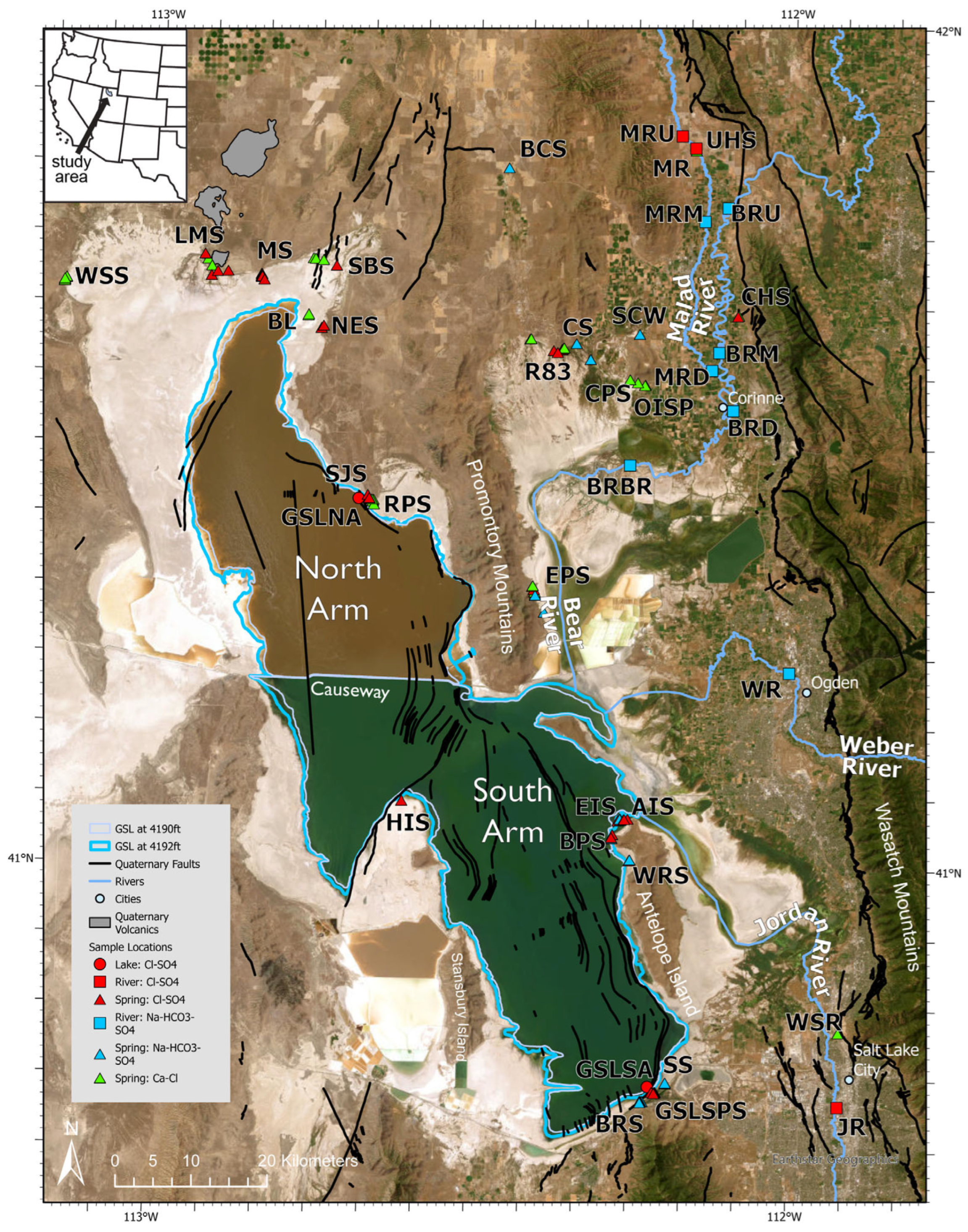
The sources of solutes to GSL are atmospheric precipitation, river water, and springs; however, atmospheric precipitation is not a significant solute source [21,38]. Three rivers enter the South Arm of GSL: the Bear River, Weber River, and the Jordan River. The Bear River flows into GSL from the north, the Weber River from the east, and the Jordan River from the south (Figure 1). The annual average river discharge between 1949 and 2010 consisted of 58% from the Bear River, with lesser contributions from the Weber River (15%) and the Jordan River (22%) [16]. Small amounts of inflow, less than 5%, are derived from other tributaries [16]. Urbanization, mining, and agriculture in the lower sections of the Bear, Weber, and Jordan Rivers make these areas susceptible to contamination and water retention [20].

Prior to construction of the earthen railroad causeway in 1959, mixing of North and South Arm brines was a function of lake elevation and flow across a fault ridge extending from Carrington Island to Promontory Point [20,36,39]. This bathymetric sill divides the South Arm into north and south sub-basins, which, at times, contain a dense brine layer (DBL) derived from bottom-flow of dense North Arm brines [36]. Low dissolved oxygen in the DBL can concentrate harmful contaminants such as methylmercury and selenium [40,41].

Mohammed and Tarboton [16] developed a mass balance model to examine lake volume changes in response to various inputs and outputs, that is, river inflow, precipitation, and evaporation. Changes in lake volume were found to be most sensitive to fluctuations in river inflow and least sensitive to fluctuations in evaporation [16]. Shope and Angeroth [42] assessed the total solute load delivered to GSL by river inflow and used the LOADEST statistical model to quantify the uncertainty in these estimates. That study did not consider spring and groundwater inflow [42].

Reports of springs surrounding GSL date back to the 1850s [43], and measurements have been made since then [22]. Spring solutes are potentially a major input to the overall salt load of GSL [20,23,33,38,44,45,46]. Springs on the east side of GSL, closest to the Wasatch Mountain front, are dominantly Ca-HCO₃ type [22]. Groundwater and rare springs on the western side of GSL, adjacent to the Bonneville Salt Flats and the West Desert, are rich in Na and Cl [22]. Hydrothermal springs to the northeast of GSL, enriched in Na, K, and Cl and with elevated δ¹⁸O, were interpreted as deeply circulated waters delivered to the surface via faults along the Wasatch mountain front [46]. A second water type, comprising most of the area’s groundwater supply, is enriched in Ca, Mg, and HCO₃ [46]. This water type is interpreted as surface runoff from lower elevations that infiltrated the shallow valley sediments [46].

Hahl [45] estimated spring inflow to GSL in 1964 to be ~2.4% of the total volume and 18.7% of the total dissolved solids [45]. Arnow and Stephens [18] estimated that 3% of the water inflow to GSL between 1931 and 1976 was groundwater. This estimate was obtained from groundwater inflow for 13 segments of the lakeshore [18]. Spencer et al. [20] and Jones et al. [21] investigated the hydrologic history of the GSL basin from lake level changes in response to inflow and outflow. Spencer et al. [20] recognized that hydrothermal springs were an important contributor to the solute load of GSL. The sources of solutes to GSL were further explored by Jones et al. [21] who proposed that inflow solutes are derived from a mixture of Ca-HCO₃ river inflow and Na-Cl hydrothermal spring inflow [21]. Kirby et al. [22] suggested that GSL must be a sink for surface and groundwater due to its location at the lowest elevation in its watershed, and that previous studies underestimated groundwater inflow volume and solute load. They compiled a groundwater database as a first step toward understanding groundwater inflow to GSL [22]. Zamora and Inkenbrandt [23] compiled existing groundwater level data to create potentiometric surface maps, calculated groundwater contributions to GSL, and estimated total solute contributions from groundwater to GSL. Using two methods, the Darcy flux equation and ArcGIS Pro spatial analysis modeling, they calculated a groundwater flux to GSL of 386.7 million cubic meters per year (313,500 acre-feet per year) and 439.1 million cubic meters per year (356,000 acre-feet per year), respectively. This is approximately 10% of the total inflow volume to GSL, much higher than previous estimates [23].

2. Methods

The locations and chemical composition of 126 water samples from springs (n = 103), rivers (n = 19), and GSL (n = 4) are shown in Figure 1 and Table S6 in the Supplementary Materials. Water samples collected in June 2021 and November 2021 were compared to determine seasonal changes in chemical composition. Discharge from 26 springs (Table S5 in the Supplementary Materials) was reported from the USGS National Water Information System: Mapper [47].

Water samples were analyzed at Binghamton University for cations, anions, alkalinity, conductivity, and density. Cations (B, Ba, Ca, Fe, K, Li, Mg, Na, and Sr) were analyzed using a Vista-MPX CCD Simultaneous ICP-OES. Some waters were diluted to produce Na concentrations within the upper range of the instrument calibration, which is about 4000 ppm. After Na and other major cations were analyzed (K, Mg, Ca), samples were analyzed undiluted for the remaining ions (i.e., B, Ba, Fe, Li, Sr). The detection limit varies for each ion on the ICP-OES (Table S3 in the Supplementary Materials). All samples analyzed were above the detection limit for all selected cations. Anions (F, Cl, Br, and SO₄) were analyzed on a Dionex ICS-2000 ion chromatograph. Samples were diluted to ensure Cl and SO₄ concentrations were in the range of instrument calibration, which is <120 ppm. Water samples were analyzed undiluted for Br and F. All concentrations are reported in parts per million (ppm). Ion concentrations measured below 1 ppm are reported as <1 ppm. Alkalinity was measured by titration. A total of 50 mL of sample was titrated to a pH of 4.50 using a Fisherbrand Accumet AB15 Basic pH meter. The titrant used was sulfuric acid solution N/50. Alkalinity was calculated using the equation:

$$\mathrm{A}\mathrm{l}\mathrm{k}\mathrm{a}\mathrm{l}\mathrm{i}\mathrm{n}\mathrm{i}\mathrm{t}\mathrm{y}={\displaystyle \frac{\mathrm{t}\mathrm{o}\mathrm{t}\mathrm{a}\mathrm{l} \mathrm{m}\mathrm{L}\ast 0.02 \mathrm{N} {\mathrm{H}}_2{\mathrm{S}\mathrm{O}}_4\ast 50000}{\mathrm{m}\mathrm{L} \mathrm{o}\mathrm{f} \mathrm{s}\mathrm{a}\mathrm{m}\mathrm{p}\mathrm{l}\mathrm{e}}}$$

(1)

Alkalinity is reported in milligrams per liter of CaCO₃. The equivalent weight of 1 mol of CaCO₃ is 50,000 mg. Density, in units of grams per milliliter (g/mL), was measured at 25 °C by weighing 10 mL of sample in an Eisco Glass Calibrated Pycnometer, using a Mettler Toledo AB104-S scale, accurate to 0.0001 g.

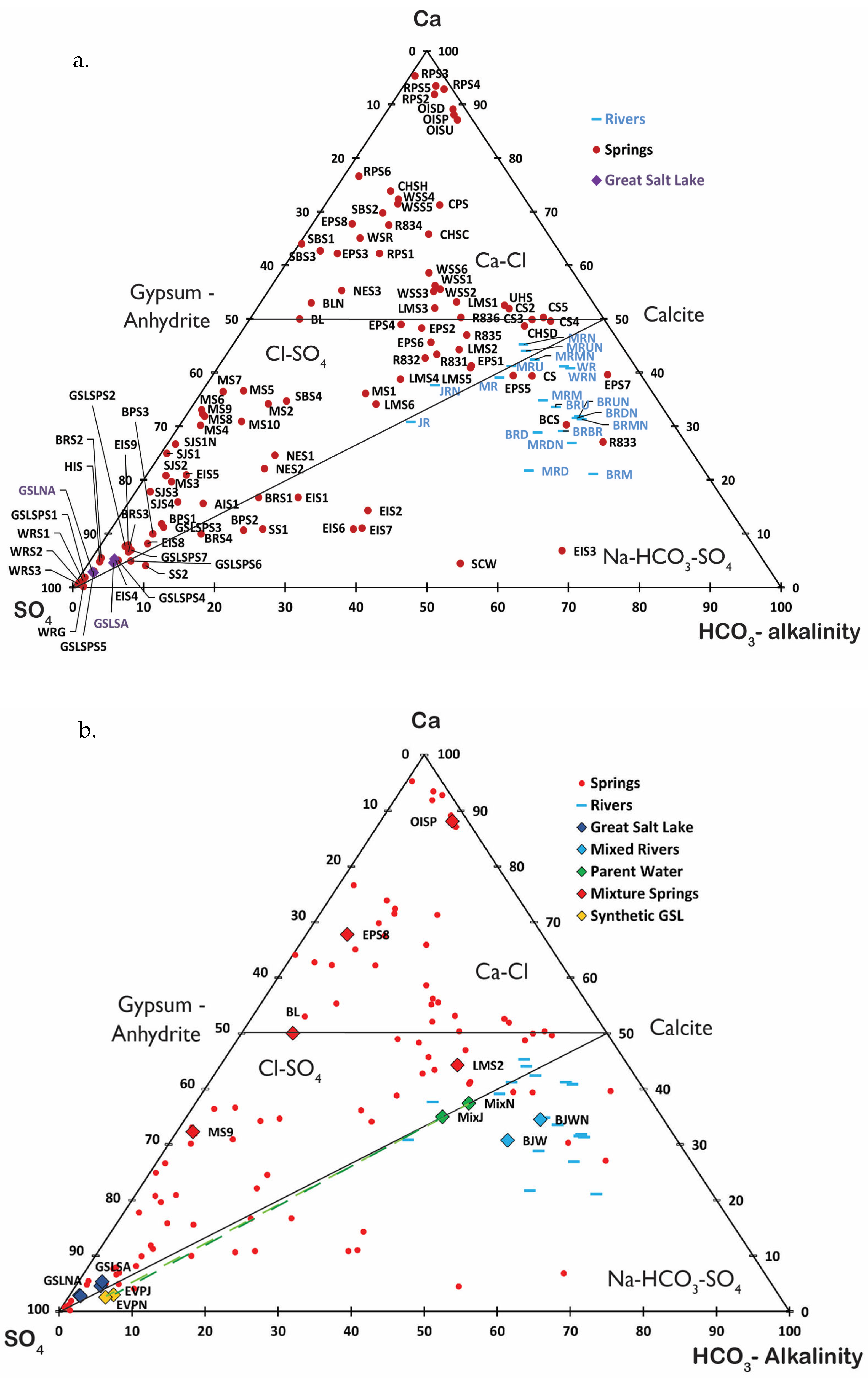
The concept of chemical divides can be used to describe the evolution of closed basin waters [21,48]. The basis of this concept is that the solubility of minerals controls mineral precipitation in evaporating waters. The ternary Ca-SO₄-alkalinity plot (Figure 2), in equivalents, can be used to predict solute evolution using the concept of chemical divides [21]. The ternary Ca-SO₄-alkalinity plot groups waters into three chemical types (Ca-Cl, Cl-SO₄, and Na-HCO₃-SO₄) defined by the CaCO₃ and CaSO₄ chemical divides. The Ca-Cl type, with equivalents of Ca > alkalinity, lies above the CaCO₃ divide and, after CaCO₃ precipitation, lies above the CaSO₄ divide, with equivalents of Ca > SO₄. The Cl-SO₄ type has SO₄ > Ca after CaCO₃ precipitation, and, thus, lies below the CaSO₄ divide, and with equivalents Ca > alkalinity, above the CaCO₃ divide. The third type, Na-HCO₃-SO₄, has Ca < alkalinity and so lies below the CaCO₃ divide.

Synthetic GSL parent waters, with Ca equal to alkalinity in equivalents, were evaporated using the Pitzer-based computer program EQL/EVP [49] to compare with the chemical composition of GSL brines from the South Arm. Such simulations tested whether the modeling used to produce the synthetic GSL parent water reproduced the concentrations of other ions in GSL brines (Na, K, Li, Mg, Cl, SO₄, and B).

3. Results

The Bear, Weber, and Jordan Rivers that discharge into GSL and the Malad River, which discharges into the Bear River, are predominantly Na-HCO₃-SO₄ waters on the ternary Ca-SO₄-alkalinity plot (Figure 2). Discharge, total dissolved solids, and chemical composition of these rivers varied seasonally and spatially. River water samples were collected in June 2021 during a period of relatively low discharge, when runoff from snow melt was minimal [50]. In November 2021, rainfall events increased discharge in the Malad, Bear, and Jordan Rivers during the sampling period.

The Bear River (BR) contributes ~58% of the average annual streamflow into GSL [16]. Samples were taken from four locations along the BR (Figure 1) to compare the chemical composition of upstream and downstream locations. The BR is a Na-HCO₃-SO₄ type water (Figure 2). The BR had an average total dissolved solids (TDS) of ~2200 ppm in June 2021. In November 2021, the average TDS was ~830 ppm. The difference between the average TDS in June and November 2021 is from rainfall events in November 2021. Upstream locations of the BR have lower TDS than the two downstream locations due to the influence of the Malad River, a tributary of the BR, which enters the BR above the downstream sites (Figure 1).

The Weber River (WR) contributes ~15% of the average annual streamflow into GSL [16]. One site was sampled in June 2021 and again in November 2021 (Figure 1). The WR has a Na-HCO₃-SO₄ composition (Figure 2) and, because it flows directly from the Wasatch Range, is the most dilute of the three rivers, with an average TDS of ~500 ppm [21].

The Jordan River (JR) contributes ~22% of the average annual streamflow into GSL [16]. One site was sampled in June and November 2021 (Figure 1). In June 2021, the JR was Na-HCO₃-SO₄ type, but in November 2021, the river was Cl-SO₄ type (Figure 2). This is due to the change in discharge from rain events in November 2021. The average TDS of the JR was ~1000 ppm.

Malad River (MR) samples were taken from two locations upstream (MRU and near the local hot springs (MR)), one from where the MR enters the BR (MRD), and a fourth site between the upstream MR locations and the MR terminus (MRM) (Figure 1). The MR is a Na-HCO₃-SO₄ type water at downstream locations and a Cl-SO₄ type at upstream locations. Ca-Cl hot springs (Uddy Hot Spring, UHS) enter the MR at upstream locations, which produces Cl-SO₄ type water with Ca > alkalinity. The Na-HCO₃-SO₄ chemical composition of the MR is produced from “contamination” by BR water that enters the lower part of the MR watershed via irrigation canals. The average TDS for the MR in June 2021 was ~3500 ppm and ~2700 ppm in November 2021, due to saline hydrothermal springs that feed the river [20]. Hydrothermal springs in the MR watershed exert an important influence on the chemical composition of the MR. The average sampled concentrations of Ca and Li in the MR, for example, were significantly higher, 109 ppm and 0.45 ppm, respectively, than in the Bear, Weber, and Jordan Rivers. The Jordan River (JR) has an average Ca concentration of 90 ppm and Li of 0.02 ppm, the Weber River (WR) has an average Ca of 68 ppm and Li of 0.002 ppm, and the BR has an average Ca of 62 ppm and Li of 0.09 ppm. Notably, the BR had a Li concentration of 0.37 ppm at the downstream site in June 2021, due to contributions from the MR. The influence of the MR and hydrothermal springs that feed into the BR can explain the increase in TDS at the downstream location (BRD) (Figure 1). The upstream (BRU) and middle stream (BRM) sites of the BR had similar TDS, 1400 ppm and 1300 ppm, respectively, in June 2021, and 630 ppm and 660 ppm, respectively, in November 2021. The downstream (BRD) site had a TDS of 3800 ppm in June and 900 ppm in November. Rain events led to the decrease in TDS of the BR between June and November 2021.

Spring waters on the perimeter of GSL (Figure 1) vary significantly in total dissolved solids. Of the 103 springs sampled, 2 had TDS < 1000 ppm, 33 had TDS between 1000 and 10,000 ppm, 29 had TDS between 10,000 and 35,000 ppm), and 39 had TDS > 35,000 ppm. Of the springs sampled, eight were hot springs with temperatures above 32 °C in June and above 25 °C in November. Springs fall into all three water types (Ca-Cl, Cl-SO₄, and Na-HCO₃-SO₄) on the ternary Ca-SO₄-alkalinity plot (Figure 2) with the majority of the springs, 85 samples, falling above the CaCO₃ divide in the Ca-Cl and Cl-SO₄ fields. Two of the springs (SJS1 and BL) were measured in June and November, bringing the total unique springs sampled to 101.

Of the 103 springs sampled, 34 are classified as Ca-Cl type springs. Ca-Cl type springs range in TDS from 1900 (i.e., CS2) to 300,000 ppm (i.e., RPS3) (Figure 2). All but one hot spring (BCS) fall in the Ca-Cl type. Hot springs are enriched in Ba, Ca, Li, and Sr. Rozel Point Spring (RPS), for example, is enriched in Ba and Sr in addition to Ca. A total of 51 springs of the 103 sampled are considered Cl-SO₄-type springs. Cl-SO₄-type springs range in TDS from 1000 ppm (i.e., CS4) to 330,000 ppm (i.e., HIS) (Figure 2). Notable Cl-SO₄ springs are Monument Springs 2–10 (MS) and Spiral Jetty springs (SJS), which are enriched in B, K, Li, and SO₄. There are 18 Na-HCO₃-SO₄-type springs ranging in total dissolved solids from 400 ppm (i.e., EPS7) to 49,000 ppm (i.e., GSLSPS6) (Figure 2). One spring in this category (WRG) lies outside the TDS range. This is likely due to evaporation. These springs are grouped with river water compositions on the ternary Ca-SO₄-alkalinity plot.

Cl-SO₄ and Na-HCO₃-SO₄-type springs that lie along the bottom of the ternary Ca-SO₄-alkalinity plot (Figure 2, i.e., SS, EIS, and GSLSPS groups) are enriched in Na and SO₄ because they mixed with GSL brine or dissolved mirabilite [51]. These springs are located on Antelope Island or near the southern shore of GSL (Figure 1). The Na-SO₄-rich springs range in TDS from 2300 ppm to 150,000 ppm (i.e., EIS3, GSLSPS1, respectively). The Na-SO₄ enrichment may be due to the 40-year lowering of lake elevation. GSL brine, which is high in SO₄ (~12,000 ppm in the South Arm), discharges as groundwater along the lake margins during rapid lake level decline [52] and may mix with groundwater in the subsurface. Elevated Na-SO₄ in springs may also result from dissolution of subsurface mirabilite. Lower lake levels have produced an increase in hydraulic head, which draws groundwater to the surface, dissolving the mirabilite, and enriching the water in Na-SO₄ [51,53]. Four SO₄-rich springs, whose compositions lie near the SO₄ apex of the ternary Ca-SO₄-alkalinity diagram (GSLSPS1, WRS1, WRS2, and WRS3), are highly enriched in SO₄ (~59,000–108,000 ppm) and precipitate mirabilite in winter when water temperatures are near 0 °C [17,51].

GSL is a Cl-SO₄-type water, whose composition lies near the SO₄ apex of the Ca-SO₄-alkalinity plot (Figure 2). GSL brine is far more concentrated than the inflow waters because the lake waters have evaporated. GSL brines range in composition seasonally and between the two arms. The North Arm is more saline than the South Arm. The North Arm had an average TDS of 330,000 ppm in June 2021 and November 2021, and the South Arm had average TDS of 170,000 ppm in June and November 2021. Samples in November 2021 were taken after GSL reached its record low of 1277.4 masl, which is reflected in the elevated concentration of dissolved species. In the North Arm, SO₄ concentration was ~25,000 ppm in June 2021 and ~27,000 ppm in November 2021, and the Ca concentration was ~320 ppm in June 2021 and ~330 ppm in November 2021. South Arm SO₄ concentration was ~12,000 ppm in June 2021 and ~12,000 ppm in November 2021 and Ca concentration was ~250 ppm in June 2021 and ~300 ppm in November 2021.

In summary, GSL brines, enriched in Cl and SO₄ and depleted in Ca and alkalinity, lie near the SO₄ apex just above the CaCO₃ divide in the Cl-SO₄ field (Figure 2) [54]. In contrast, river waters plot below the CaCO₃ divide in the Na-HCO₃-SO₄ field. Evaporation of river waters would produce alkaline brines enriched in HCO₃ and SO₄ and depleted in Ca [54]. The alkalinity of GSL is low, so the chemical compositions of river waters are on the wrong side of the CaCO₃ chemical divide to evolve into GSL brines following evaporation. The mixing of Ca-Cl spring water and river inflow, thus, must play an important role in producing the composition of GSL.

3.1. Mixing Model

The goal of the model is to construct a hybrid water composed of a mixture of river and spring waters entering GSL that, when evaporated, has the chemical composition of GSL brine. The chemical composition of this “synthetic” GSL parent water is constrained by the principle of chemical divides as illustrated by the ternary Ca-SO₄-alkalinity plot (Figure 2). The chemical composition of GSL brine lies near the SO₄ apex, with low but nearly equal concentrations of Ca and alkalinity, approximately on the Ca-SO₄ join (Figure 2). A synthetic spring-river water mixture was, thus, selected (Figure 2b) whose composition fell on the CaCO₃ chemical divide (the Ca-SO₄ join). Such water, when evaporated, will precipitate CaCO₃ (aragonite) and evolve into a brine with concentrations of Ca, SO₄, and alkalinity similar to GSL brine. The input used for producing the synthetic GSL parent water is the chemical composition of all rivers and springs entering GSL and their measured discharges.

3.2. River Water Inflow

The relative contribution of the Bear, Jordan, and Weber Rivers to GSL was calculated using stream discharge data (cubic feet per second, cfs) from the USGS National Water Information System: Mapper [47]. The stations chosen for stream flow data are downstream sample sites because they reflect the most accurate discharge of each river. The BR discharge station (USGS 10126000 Bear River near Corinne, UT, USA) has stream flow data from 4 November 1949 to present (17 February 2022 for this report). The average discharge of the BR from 1949 to 2022 was 1794 cfs. The WR discharge station (USGS 10137000 Weber River at Ogden, UT, USA) has stream flow data from 12 May 2016 to present (28 January 2022 for this report). The average discharge of the WR between 2016 and 2022 was 546 cfs. Last, the Jordan River station (USGS 10170500 Surplus Canal at Salt Lake City, UT, USA) has stream flow data from 14 October 1980 to present (14 February 2022 for this report). The average discharge of the JR from 1980 to 2022 was 675 cfs. The total average river discharge into GSL is ~3015 cfs. Using this average discharge, the BR contributes 60% of total river inflow, and the WR and JR contribute 18% and 22%, respectively.

To construct the synthetic GSL parent water for this model, aliquots of the BR, WR, and JR were mixed, using their average discharge, to produce a synthetic river water representative of the total river inflow into GSL in terms of composition and volume. River inflow composition for each ion in the synthetic GSL parent water was calculated from:

$$C_{mix}={\displaystyle \frac{\left(C_{\mathrm{B}\mathrm{e}\mathrm{a}\mathrm{r}}\ast d_{\mathrm{B}\mathrm{e}\mathrm{a}\mathrm{r}}\right)+\left(C_{\mathrm{W}\mathrm{e}\mathrm{b}\mathrm{e}\mathrm{r}}\ast d_{\mathrm{W}\mathrm{e}\mathrm{b}\mathrm{e}\mathrm{r}}\right)+(C_{Jordan}\ast d_{Jordan})}{d_{\mathrm{B}\mathrm{e}\mathrm{a}\mathrm{r}}+d_{\mathrm{W}\mathrm{e}\mathrm{b}\mathrm{e}\mathrm{r}}+d_{Jordan}}}$$

(2)

$C_{mix}$ = concentration (equivalents) of ion in synthetic river water;

$C_n$= concentration (equivalents) of ion from source water n;

$d_n$ = discharge (cubic feet per second) from river water n.

Two river mixtures were prepared for the model using compositions from June 2021 and November 2021 (

Table 1. Sample calculation showing the composition (milliequivalents) and discharge (cubic feet per second) of the river mixtures (June 2021 and November 2021) and springs used to calculate GSL parent waters. The variables d_n, f_n, and X_n are measured discharge (cfs), spring factor (f_n), and weighted spring discharge (cfs), respectively.

		B3+	Ba2+	Ca2+	K+	Li+	Mg2+	Na+	Sr2+	Cl−	SO42+	Alk	dn	fn	Xn	%
June	BL	2.45	0.001	36.7	27.0	0.84	44.9	1016	0.50	1101	31.6	5.16	0.22	35	7.80	12
	MS9	3.80	0.001	25.2	30.3	0.93	86.3	1201	0.28	1198	51.1	1.72	0.89	111	99.0
	OISP	1.07	0.05	38.0	10.4	0.42	26.9	357	0.58	435	0.92	4.22	0.06	29	1.7
	EPS8	0.76	0.001	41.2	7.56	0.30	28.6	376	0.34	400	16.2	3.40	0.69	95	66.0
	LMS2	0.12	0.001	5.68	1.87	0.05	6.44	38.5	0.08	54.2	2.99	4.16	23.1	11	254
	River Mixture	0.11	0.001	3.65	1.03	0.03	4.17	32.7	0.03	35.0	2.76	5.47	3015	1	3015	88
	GSL Parent Water	0.24	0.001	5.23	2.12	0.07	7.26	75.6	0.05	79.3	4.49	5.23	3040		3443	100
November	BL	2.45	0.001	36.7	27.0	0.84	44.9	1016	0.50	1101	31.6	5.16	0.22	20	4.46	10
	MS9	3.80	0.001	25.2	30.3	0.93	86.3	1201	0.28	1198	51.1	1.72	0.89	95	84.6
	OISP	1.07	0.05	38.0	10.4	0.42	26.9	357	0.58	435	0.92	4.22	0.06	17	1.0
	EPS8	0.76	0.001	41.2	7.56	0.30	28.6	376	0.34	400	16.2	3.40	0.69	82	56.6
	LMS2	0.12	0.001	5.68	1.87	0.05	6.44	38.5	0.08	54.2	2.99	4.16	23.1	8.7	201
	River Mixture	0.04	0.001	3.73	0.34	0.003	3.11	6.49	0.01	6.09	1.82	5.25	3015	1	3015	90
	GSL Parent Water	0.16	0.001	5.07	1.34	0.03	5.89	46.1	0.03	47.1	3.42	5.07	3040		3363	100

). The two mixtures show seasonal differences in river water chemistry. The same average discharge for each river was used for the June and November mixtures

3.3. Spring Inflow

Spring discharge in the vicinity of GSL was obtained from the USGS National Water Information System: Mapper [47]. Of the 101 unique springs sampled in this study, 27 springs had measured discharges (Table S5 in the Supplementary Materials). Five springs with relatively high discharge were chosen to represent the spring inflow component of the synthetic GSL parent water (Table 1 and Figure 3). SO₄-rich springs were not considered in the modeling because they are derived from GSL water or from dissolved subsurface mirabilite. The composition of these SO₄-rich springs is, thus, not representative of inflow to GSL.

• Old Indian Hot Spring (OISP) (Figure 1, Figure 2 and Figure 3). OISP is a warm (38.3 °C) Ca-Cl-type water enriched in Na, Ba, Ca, Sr, and Cl, with TDS of ~25,400 ppm, and measured discharge of 0.06 cfs on 24 May 1966 (USGS 413437112135701 (B-10-3)30bbd-S1).
• East Promontory Spring 8 (EPS8) (Figure 1, Figure 2 and Figure 3) is a Ca-Cl-type water enriched in Na, Ca, K, Mg, Cl, and SO₄, with a TDS of 25,300 ppm and measured discharge of 0.69 cfs on 1 October 1963 (USGS 412010112242201 (B-7-5)15cba-S1).
• Locomotive Springs 2 (LMS2) (Figure 1, Figure 2 and Figure 3) is a Cl-SO₄-type water, enriched in Na, Ca, and Cl, with a TDS of ~3400 ppm and measured discharge 23.1 cfs on 1 May 1971 (USGS 414315112562001 (B-12-10)36cab-S1).
• Monument Spring 9 (MS9) (Figure 1, Figure 2 and Figure 3) is a Cl-SO₄ type water, enriched in Na, Ca, K, Mg, Cl, and SO₄, with TDS of ~75,600 ppm and discharge of 0.89 cfs on 1 August 1963 (USGS 414154112502801 (B-11-9)10ada-S1
• Blue Lagoon (BL) (Figure 1, Figure 2 and Figure 3) is a Ca-Cl-type water enriched in Na, Ca, Mg, K, Cl, SO₄, and Li with TDS of ~66,500 ppm and measured discharge of 0.22 cfs in August 2021 (The Utah Geological Survey).

3.4. Mixing

Weighted river water inflow and five spring waters (Table 1) were mixed to construct a synthetic spring–river parent water whose composition lies exactly at the CaCO₃ chemical divide, with equivalents Ca = alkalinity. The following equation was used with springs Blue Lagoon (BL), Monument Spring 9 (MS9), Old Indian Spring Pool (OISP), East Promontory Spring 8 (EPS8), and Locomotive Spring 2 (LMS2):

$$C_{mix}={\displaystyle \frac{\left(C_{\mathrm{B}\mathrm{L}}\ast X_{\mathrm{B}\mathrm{L}}\right)+\left(C_{\mathrm{M}\mathrm{S}9}\ast X_{\mathrm{M}\mathrm{S}9}\right)+\left(C_{OISP}\ast X_{OISP}\right)+\left(C_{EPS8}\ast X_{EPS8}\right)+\left(C_{LMS2}\ast X_{LMS2}\right)+(C_{River}\ast X_{River})}{X_{\mathrm{B}\mathrm{L}}+X_{\mathrm{M}\mathrm{S}9}+X_{OISP}+X_{EPS8}+X_{LMS2}+X_{River}}}$$

(3)

$C_{mix}$ = concentration (eq) of ion in synthetic GSL parent water;

$C_n$= concentration (eq) of ion in source water n;

$X_n$ = weighted discharge (cfs) from source water n.

Ionic concentrations and discharges for the synthetic river water and spring waters are listed in Table 1. Mixing of the synthetic river and spring waters, with their measured discharges (Equation (3)), did not yield a parent water with equivalents of Ca equal to alkalinity. A factor, f_n, was, thus, needed for each spring to ensure that the calculated GSL parent water mixture had equal equivalents of Ca and alkalinity (Table 1). The following equation was used to calculate the weighted discharge for each spring water:

$$X_n=d_n\ast f_n$$

(4)

$X_n$ = weighted discharge (cfs) from source water n;

$d_n$ = measured discharge from source water n;

$f_n$ = multiplication factor for source water n used to calculate the total discharge ($X_n$) from source water n into synthetic GSL parent water.

The river mixture multiplication factor, f_n, was set to 1 because the total river inflow into GSL is known. The f_n factors for each spring inflow (f_BL, f_MS9, f_OISP, f_EPS8, and f_LMS2) were initially set to 30 and then adjusted in Equation (4) to yield a calculated GSL parent water with equal equivalents of Ca and alkalinity, which was 5.23 and 5.07 milliequivalents for the June 2021 and November 2021 datasets, respectively (Table 1). The factoring process considered the discharge and composition of each spring. The f_n results are one of many possible combinations of spring inflows but nonetheless are considered representative of the diverse chemical compositions of spring inflow to GSL.

The calculations used to obtain the chemical composition of the synthetic GSL parent waters (June 2021 and November 2021) are shown in Table 1. Volume percentages (%) were calculated using the weighted discharge of the springs and rivers (Table 1):

$$Volume\%={\displaystyle \frac{X_n}{X_{Total}}}\ast 100$$

(5)

X_n = weighted discharge (cfs) of spring or river;

X_Total = total weighted discharge (cfs) in synthetic GSL parent water.

The total calculated discharge for the June 2021 synthetic parent water is 3443 cfs; 3015 cfs (88%) from rivers and 428 cfs (12%) from springs (Table 1). The synthetic GSL parent water calculated for the November 2021 river inflow composition has a total discharge of 3363 cfs, with 3015 cfs (90%) from rivers and 348 cfs (10%) from springs (Table 1).

The relative contributions of solutes from rivers and springs in the synthetic GSL inflow mixture, in percent, was calculated by converting solute concentrations in spring, river, and the synthetic GSL parent water from milliequivalents to moles (Equations (S1)–(S3) in Supplementary) and then using Equation (6):

$$Molar\%={\displaystyle \frac{C_n}{C_{Total}}}\ast 100$$

(6)

C_n = moles of solute in spring or river inflow waters;

C_Total = moles of solute in synthetic GSL parent water.

The solute percentage calculations show that on a molar basis, >50% of the B, K, Li, Na, and Cl in the synthetic GSL parent water is supplied by springs and >50% of the Ba, Ca, Sr, SO₄, and alkalinity is derived from rivers (June 2021) (

Table 2. Solute load (molar %) for each ion from springs and rivers calculated for synthetic GSL parent water (June and November 2021).

		B3+	Ba2+	Ca2+	K+	Li+	Mg2+	Na+	Sr2+	Cl−	SO42−	Alk
June	Springs	58	15	29	57	57	50	62	44	61	46	8
	Rivers	42	85	71	43	43	50	38	56	39	54	92
November	Springs	77	9	34	77	93	53	87	59	88	52	7
	Rivers	23	91	66	23	7	47	13	41	12	48	93

). Springs supply the bulk of the Na and Cl to GSL, whereas rivers supply most of the alkalinity.

3.5. Evaporation

The goal of the mixing model was to construct a synthetic GSL parent water that, when evaporated, had a chemical composition similar to the South Arm of GSL. The South Arm brines were chosen over the North Arm brines because of their lower salinity, below saturation with respect to halite. Thus, Cl is a conservative component in South Arm brines and is not lost from the synthetic GSL parent water during the modeled evaporation. South Arm brines have a Cl concentration of 2600 mmol/kg H₂O. The synthetic spring–river parent water was, therefore, evaporated to a Cl concentration of 2600 mmol/kg H₂O so that the ions in the synthetic GSL parent water (Na, K, Li, Mg, SO₄, and B) could be compared to the those in GSL South Arm brine at the same Cl concentration.

The compositions of the June 2021 and November 2021 synthetic GSL parent waters are listed in Table 1 and plotted on Figure 2. The composition of the synthetic GSL parent waters was intentionally computed to lie exactly on the CaCO₃ chemical divide, that is, with equal equivalents of Ca and alkalinity (Figure 2). The composition reflects the low, subequal concentrations of Ca and HCO₃ in GSL brines. Precipitation of aragonite removes Ca and CO₃ from the evaporating brine in equal molar proportions, which is expressed on the ternary Ca-SO₄-alkalinity diagram by a path directly away from the CaCO₃ composition toward the SO₄ apex.

The June 2021 and November 2021 synthetic GSL parent waters were evaporated using EQL/EVP at atmospheric pCO₂ of 10^−3.4, pH of 7.9, and 18 °C, and the temperature of the South Arm of GSL in June 2021 are presented in

Table 3. Chemical compositions (mmol/kg H₂O) of measured GSL South Arm brines and June 2021 and November 2021 synthetic parent waters after evaporation under closed conditions at 18 °C and 30 °C.

		B3+	Ca2+	K+	Li+	Mg2+	Na+	Cl−	SO42−	Alk
South Arm		2.30	6.50	86.0	3.10	240	2200	2600	130	4.90
June	18 °C	2.57	2.35	68.4	2.12	117	2446	2608	71.6	4.71
	30 °C	2.57	2.12	68.4	2.12	117	2446	2608	71.6	4.25
November	18 °C	2.76	2.51	72.0	1.89	158	2400	2607	91.5	5.03
	30 °C	2.76	2.28	72.0	1.89	158	2400	2607	91.5	4.55

. The only alkaline earth carbonate currently forming in GSL today is aragonite, so precipitation of all other carbonates (calcite, dolomite, magnesite, hydromagnesite, and nesquehonite) was suppressed. The chemical compositions of the synthetic GSL parent waters were not changed when evaporated under open (no back reactions between precipitated minerals and brine) versus closed conditions (back reactions allowed) [49] because the only mineral precipitated during evaporation simulations up to GSL South Arm Cl concentrations was aragonite. Mirabilite forms today as a low temperature salt from GSL South Arm brines during the winter months, and indeed it precipitated when the synthetic GSL parent waters were evaporated at low temperatures (i.e., 5 °C). But mirabilite is dissolved back into GSL brines during spring and summer, so it was not considered in the evaporation model. The GSL parent waters were also evaporated at 30 °C to determine what influence aragonite, with lower solubility at high temperature, has on the chemical composition of the evaporated synthetic parent water mixture. Evaporation of the synthetic GSL parent water (June 2021 composition) at 30 °C to the current Cl molality of the GSL South Arm lowered Ca²⁺ and alkalinity by 12.5% (2.12 mmol/kg H₂O of Ca²⁺ at 30 °C versus 2.35 mmol/kg H₂O at 18 °C) and 11% (4.25 mmol/kg H₂O at 30 °C versus 4.71 mmol/kg H₂O at 18 °C), respectively, and did not influence any of the other major and minor ions. Thus, evaporation simulations at 18 °C were considered sufficient (Table 3). The degree of evaporation (DE: concentration of a solute after evaporation divided by initial concentration of a solute) needed to reach the Cl molality of South Arm brine was 33 and 54, respectively, for the June 2021 and November 2021 GSL parent waters.

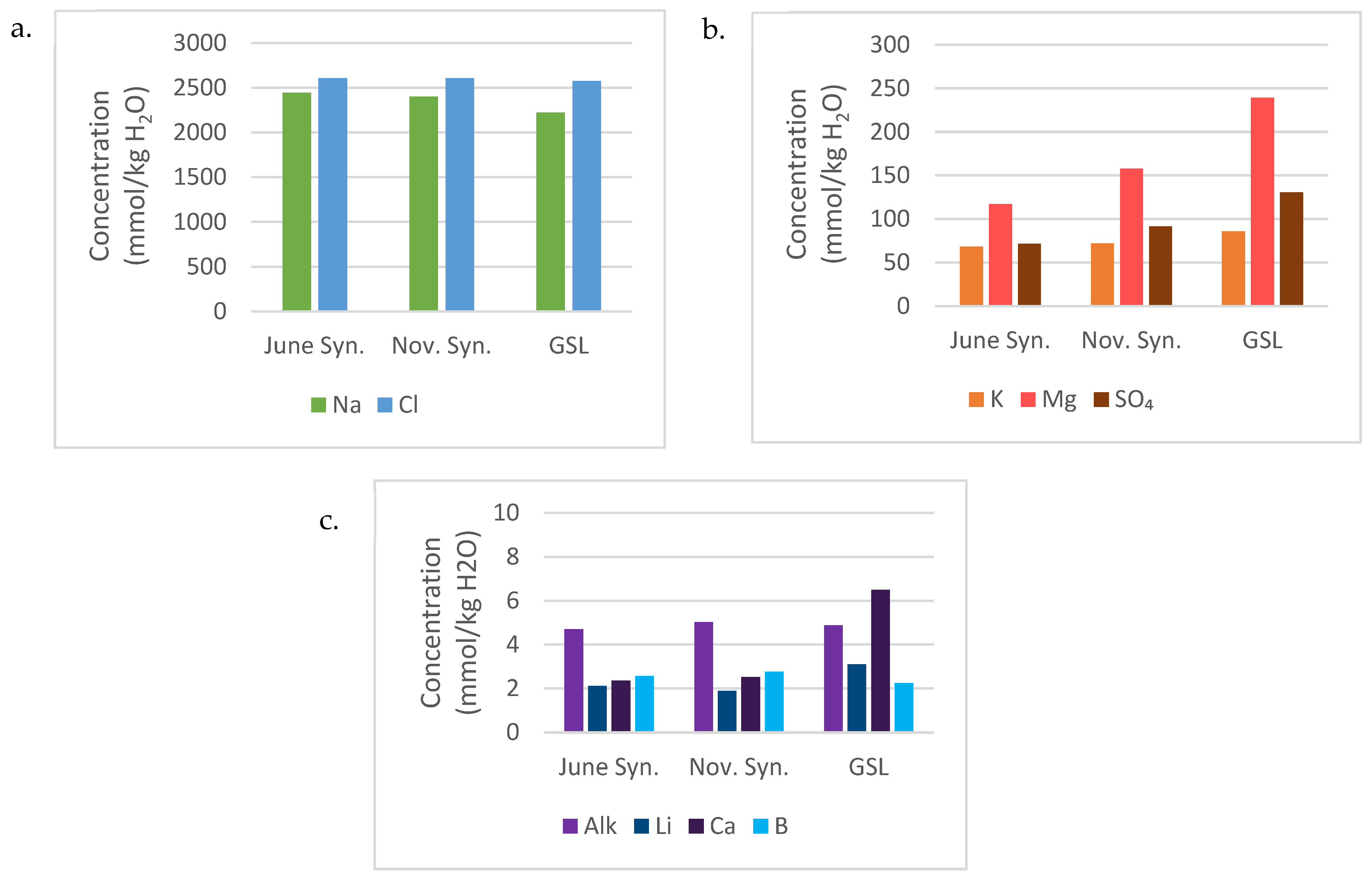
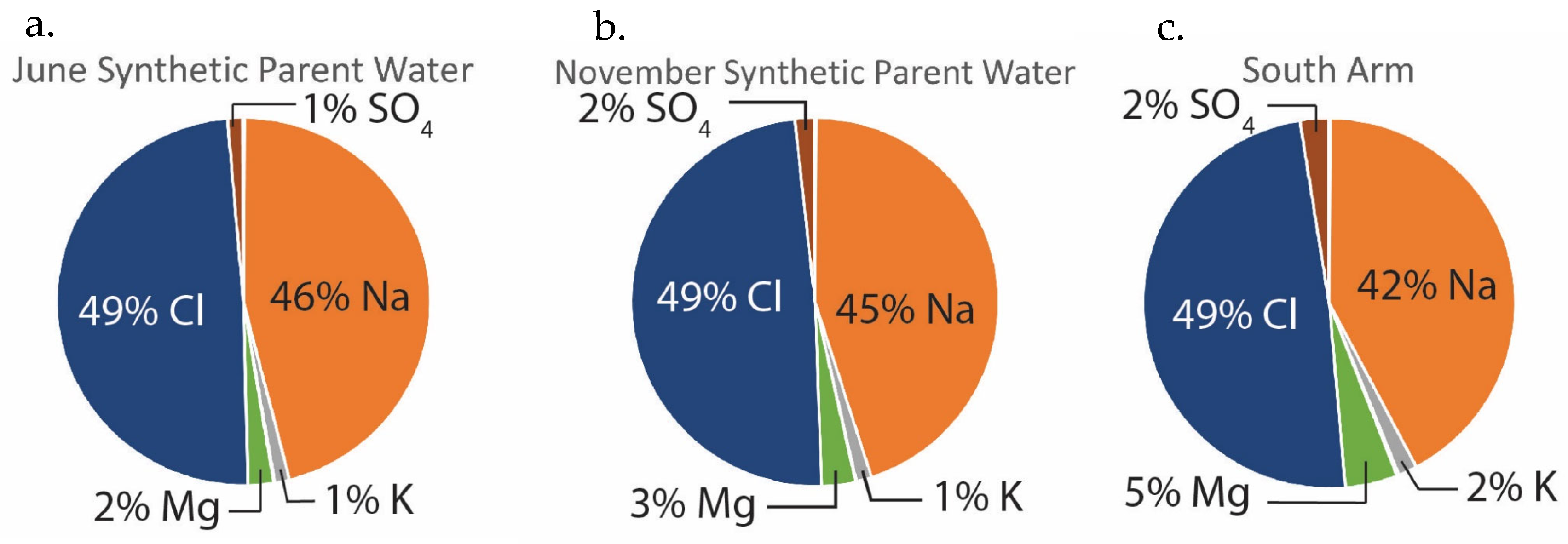
Evaporated June and November 2021 synthetic parent waters are compared to GSL South Arm brine composition (Table 3) and plotted by major (Na and Cl), minor (K, Mg, and SO₄), and trace (alkalinity, Li, Ca, and B) ions (Figure 4). The relative ionic concentrations in the evaporated June and November synthetic parent waters are compared to the chemical composition of the GSL South Arm brine in Figure 5. Evaporated synthetic parent waters and GSL South Arm brines share the following characteristics:

• Na (2200 to 2446 mmol/kg H₂O) and Cl (~2600 mmol/kg H₂O) are the dominant species, in all cases comprising > 90% of the total dissolved solids (Figure 4a and Figure 5).
• Mg (117 to 240 mmol/kg H₂O), SO₄ (72 to 130 mmol/kg H₂O) and K (68–86 mmol/kg H₂O) comprise 4 to 9% of the total dissolved solids, with Mg > SO₄ > K (Figure 4b and Figure 5).
• Ca and alkalinity are significant species in inflow waters (Table 1) but become trace ions with subequal concentrations due to precipitation of aragonite during evaporation (Ca: 2.1 to 6.5 mmol/kg H₂O; alkalinity: 4.3 to 5.0 mmol/kg H₂O) (Figure 4c).
• Trace ion concentrations, for example, Li (1.9 to 3.1 mmol/kg H₂O) and B (2.3 to 2.8 mmol/kg H₂O) in evaporated parent waters are close to those found in GSL South Arm brine (Figure 4c).

Such comparisons are considered significant and lead to the conclusion that the river and spring water inflows used in the model are reasonable. Further refinement of the modeling is not justified because of the numerous uncertainties and assumptions, including the following:

• Incomplete sampling of total possible number of springs that supply solutes to GSL.
• Springs chosen may not be completely representative of the total spring discharge to GSL, in terms of discharge and chemical composition; corrections such as weighted spring discharge and spring factor were needed to produce a spring mixture that, when mixed with river water and evaporated, yielded GSL brine chemical composition.
• Modern river and spring inflow chemical compositions and discharges are influenced by industry (mining), agriculture, and urbanization.
• Discharge data are available for only 27 springs (Table S5).

4. Discussion

Previous studies contributed to expanding the knowledge of the GSL geochemical system by describing spring and groundwater inflows. Spencer et al. [20] created a hydrochemical model for GSL, which suggested that the primary natural inputs are atmospheric precipitation, river waters, and hydrothermal springs. The study concluded that hydrothermal springs are significant contributors of dissolved species to GSL [20]. Loving et al. [33] revised the Wold et al. [37] water and salt balance model for GSL and suggested that changes in lake level occur in response to the balance between evaporation and inflow from a combination of runoff, groundwater, and direct precipitation. That study estimated groundwater to be a small contributor to the overall inflow into GSL [33] but used limited data from piezometers, high resolution sentinel imagery modeling, and geophysical surveys. Jones et al. [21] tudied the geochemical evolution of GSL and suggested that the major dissolved constituents could be approximated by mixing dilute calcium bicarbonate-rich stream waters with NaCl-dominated groundwaters and hydrothermal springs.

Kirby et al. [22] created the first systematic basin-wide assessment of groundwater chemistry in the GSL area by providing a comprehensive ArcGIS format geodatabase of groundwater samples. The study suggested that GSL groundwater quantity and quality need to be better defined. The database shows that the west shore of GSL is predominantly Na-Cl type groundwater whereas the east shore is Ca-HCO₃ type groundwater. Kirby et al. [22] suggested that a mixing model could be produced, using the database, to estimate the probable quantity of groundwater that contributes to GSL, but potentiometric surfaces, spring locations, and flow rate measurements are needed.

Zamora and Inkenbrandt [23] provided a systematic, basin-wide assessment of groundwater levels near GSL in order to quantify groundwater contributions to the lake. Using two independent models (Darcy flux and ArcGIS Pro spatial analysis modeling), they arrived at a similar conclusion to this study, that groundwater contributes greater than ~10% of the total inflow by volume to GSL [23].

Here, the parent water chemistry for GSL was assembled using 5 spring types and a mixture of Bear River, Weber River, and Jordan River waters. Spring waters (Ca-Cl and Cl-SO₄ types) mixed with river water (Na-HCO₃-SO₄) produced a parent water, which, when evaporated, evolved to a brine similar in composition to the modern chemical composition of the South Arm of GSL. That model shows that springs contribute 10–12% by volume to GSL, which is 3–4 times greater than the 3% estimate by Arnow and Stephens [18]. The mixing model presented here shows that spring waters contribute, on a molar basis, greater than 50% of the B, K, Li, Na, and Cl to GSL. River water contributes greater than 50% of the Ba, Ca, Sr, SO₄, and alkalinity on a molar basis to the GSL.

4.1. The Future of Great Salt Lake

Great Salt Lake, as a closed basin lake, is sensitive to climate change. Over the past decade, extended drought combined with development and consumptive use, has reduced lake levels by about 3.4 m [10,16]. Without development and consumptive use, GSL was modeled to have a natural mean elevation of 1282 masl, which is 5.4 m higher than the record low recorded in November 2022 (1276.6 masl) [2,8,9]. Future development of the Bear River is being considered by the States of Utah, Idaho, and Wyoming that could lower lake level more than 1.6 m [15]. Continued development and consumptive use of water will lower the river and spring inflow into GSL [55]. The reduced inflow from the Bear River, and the greater influence of springs will impact the future composition of GSL.

Diversion of inflow waters to GSL will modify the hydrological balance of the system, especially as climate change creates a warmer and drier regional climate there [56]. Understanding spring inflow to GSL is, therefore, important for the development of water management programs [42]. Groundwater influence on the salt budget in GSL has important implications for the wildlife and industries that rely on the lake. Wetland habitats, brine shrimp, and mineral extraction industries all rely on differing levels of salinity.

Increased pumping of fresh groundwater aquifers will decrease the amount of dilute groundwater entering GSL [31] and will have a negative effect on the wetland habitats around GSL. Locomotive Springs (LMS2 on Figure 1 and Figure 3c) is one example of the decline of wetlands due to human consumption. The discharge from this spring system has steadily decreased from 40 cubic feet per second in the 1960s to less than 10 cubic feet per second in the early 2000s [31]. Locomotive Springs provide a habitat for migratory birds as part of the Utah State Waterfowl Management Area, but decreased spring discharge has led to a decline in wetland acreage since the mid-1980s. Vegetated and water-covered functional wetlands have been replaced by an increasing area of dry mudflats, which has resulted in decreased waterfowl visitation to the area [31].

Increasing salinity of GSL would negatively impact the brine shrimp population. Brine shrimp can tolerate salinities up to approximately ~20%. Salinities > ~20% stress the brine shrimp community, which leads to reproductive failure and population decline [15,55,57]. This decline would have serious impacts on the migratory bird population, which relies on brine shrimp for food, and the $57 million dollar brine shrimping industry at GSL [55].

The decrease in GSL level positively impacts the mineral extraction industry by concentrating brines and shortening the evaporation process [55]. However, there are also negative impacts. Lower lake levels make GSL increasingly difficult to navigate by boat, hindering mining company access to the brine ponds, at lake elevations < 1278.6 masl [2,55,56]. For example, Morton Salt constructed an eight-kilometer-long canal in 2014 to enable water access [55].

4.2. Improvements in the Model

The mixing model of spring and river waters presented here is a first step in understanding the impact of spring inflow to GSL. In order to improve the model, additional spring discharge measurements and spring compositional data are needed. Of the 101 unique springs sampled in this study, only 27 had recorded discharge measurements. Most of those measurements were taken by the USGS in the 1960s and 1970s. Changes in groundwater flow due to diversion and human consumption have changed groundwater discharge over the last half century. For example, the total flow from Locomotive Springs averaged approximately 33 cfs from 1969 to 1972 but declined to an average of 14 cfs from 1993 to 1996 [58].

The spring compositions analyzed in this study are generally assumed to be representative of the differing water types entering GSL. Increasing the database of spring chemical compositions and their discharge would more quantitatively define spring contributions to the GSL system. Additional measurements, such as the δ¹⁸O [46] and Sr isotopic composition [59] of springs and river inflow might better constrain their relative contributions to producing the chemical composition of Great Salt Lake.

5. Conclusions

The chemical compositions of GSL, the Bear, Jordan, and Weber Rivers, and 103 springs were determined in this study. The compositions were separated into distinct water types based on the ternary Ca-SO₄-alkalinity plot. Five springs with relatively high discharge were chosen to represent the spring inflow component of the synthetic GSL parent water:

• Old Indian Hot Spring (OISP) represents Ca-Cl type waters enriched in Na, Ba, Ca, Sr, and Cl;
• East Promontory Spring 8 (EPS8) represents Ca-Cl type waters enriched in Na, Ca, K, Mg, Cl, and SO₄;
• Locomotive Springs 2 (LMS2) represents Cl-SO₄ type waters enriched in Na, Ca, and Cl;
• Monument Spring 9 (MS9) represents Cl-SO₄ type waters enriched in Na, Ca, K, Mg, Cl, and SO₄;
• Blue Lagoon (BL) represents Ca-Cl type waters enriched in Na, Ca, Mg, K, Cl, SO₄, and Li.

A synthetic GSL parent water was used to calculate the relative inflow percentages needed from springs and rivers to produce current GSL brine chemistry. The mixing model shows that a synthetic parent water produced by mixing of springs and river water yielded inflow volume percentages of 88–90% for rivers and 10–12% for springs. Springs contribute more than 50% of B, K, Li, Na, and Cl to GSL on a molar basis. Evaporation of the synthetic GSL parent water using the Pitzer-based computer program EQL/EVP [49] reproduced GSL brine concentrations in the South Arm. Na, Cl, K, Mg, SO₄, alkalinity, Li, Ca, and B concentrations in evaporated synthetic parent waters showed only small differences from the GSL South Arm brine composition. The importance of understanding the contribution of groundwater to GSL is highlighted by its recent historic low level. With decreasing surface water discharge into the lake, groundwater inflow becomes increasingly important for maintaining GSL. With increased knowledge of groundwater inflow into the lake, better mitigation and land-management plans can be put into place to help protect the wildlife and the industries that rely on GSL.