Article

Impact of Spatio-Temporal Variability of Droughts on Streamflow: A Remote-Sensing Approach Integrating Combined Drought Index

by
Anoma Srimali
1,
Luminda Gunawardhana
1,2,
Janaka Bamunawala
3,*,
Jeewanthi Sirisena
4 and
Lalith Rajapakse
1,2
1
Department of Civil Engineering, University of Moratuwa, Katubedda 10400, Sri Lanka
2
UNESCO-Madanjeet Singh Centre for South Asia Water Management (UMCSAWM), University of Moratuwa, Katubedda 10400, Sri Lanka
3
Department of Civil and Environmental Engineering, Graduate School of Engineering, Tohoku University, Sendai 980-8579, Japan
4
Climate Service Center Germany (GERICS), Helmholtz-Zentrum Hereon, 20095 Hamburg, Germany
*
Author to whom correspondence should be addressed.
Hydrology 2025, 12(6), 142; https://doi.org/10.3390/hydrology12060142
Submission received: 30 April 2025 / Revised: 1 June 2025 / Accepted: 3 June 2025 / Published: 7 June 2025

Abstract

Understanding how spatial drought variability influences streamflow is critical for sustainable water management under changing climate conditions. This study developed a novel Combined Drought Index (CDI) and a method to assess spatial drought impacts on different flow components by integrating remote sensing and hydrological modelling frameworks with generic applicability. The CDI was constructed using Principal Component Analysis to merge multiple standardized indicators: the Standardized Precipitation Evapotranspiration Index, Temperature Condition Index, Vegetation Condition Index, and Soil Moisture Condition Index. The developed framework was applied to the Giriulla sub-basin of the Maha Oya River Basin, Sri Lanka. The CDI strongly correlated with standardized streamflow with a Pearson correlation coefficient of 0.74 and successfully captured major drought and flood events between 2015 and 2023. A semi-distributed hydrological model was used to simulate streamflow variations across sub-catchments under varying drought conditions. Results show upstream sub-catchments were more sensitive to droughts, with sharper declines in specific discharge. Spatial drought variability had different impacts under high- and low-flow conditions: wetter sub-catchments contributed more during high flows, while resilience during low flows varied with catchment characteristics. This integrated approach provides a valuable framework that can be generically applicable for enhanced drought impact assessments.

1. Introduction

Drought is identified as a prolonged absence or marked deficiency of precipitation that results in a significant water shortage [1]. Globally, droughts represent one of the most far-reaching and damaging natural hazards, contributing to widespread economic, environmental, and social consequences [2,3,4,5,6,7,8]. While these widespread consequences manifest across all socio-economic sectors of society, the agricultural sector’s vulnerability particularly stands out, with drought identified as the foremost cause of productivity losses in crops and livestock within the drought-affected regions and beyond [3,4]. While droughts affect populations worldwide, low- and middle-income countries, such as Sri Lanka, experience disproportionate impacts due to their heavy dependence on climate-sensitive sectors like agriculture and limited institutional capacity for mitigation and adaptation [8]. Table 1 summarizes key statistics and projections on drought impacts drawn from authoritative global and regional sources, highlighting the differential burden experienced by vulnerable economies.
Droughts can arise from a complex interplay of natural climatic variability and anthropogenic influences. Prolonged deficits in precipitation, elevated temperatures, and changes in atmospheric circulation patterns are the key natural drivers that disrupt the hydrological cycle, reducing soil moisture, streamflow, and groundwater recharge [9,10]. This relationship is evident in studies showing that increased precipitation deficits correspond to more severe and less frequent droughts, reflected in distinct severity—duration—frequency patterns [11]. Moreover, the rise in actual evapotranspiration has been identified as a key trigger for seasonal droughts, showing a strong negative spatial correlation with related indices such as the Standardized Precipitation Evapotranspiration Index (SPEI) [12], highlighting its role in intensifying water scarcity under changing climate conditions. In addition, recent research (e.g., [13,14]) suggests a weakening trend in the South Asian summer monsoon over the past decades, influenced by broad-scale ocean-atmosphere interactions and climate system variability. Projected changes in the climatic conditions over the 21st century are expected to amplify these dynamics by increasing rainfall irregularity [13,14], shifting precipitation timing and intensity [15,16] and enhancing atmospheric demand for moisture [17,18], factors that collectively heighten the frequency and severity of drought episodes across the region [19].
In addition to climatic factors, human-induced changes such as rapid urbanization, water diversions, and land-use transformation significantly contribute to intensifying the drought impacts [20]. Expanding urban areas, deforestation, and converting natural landscapes into agriculture or built-up land alter the land surface energy balance [21,22] and hydrological processes [23]. These changes may lead to diminished groundwater recharge and soil moisture retention, making ecosystems and water supply systems more vulnerable during dry periods [24]. Furthermore, growing water demand from agricultural, industrial, and domestic sectors exacerbates water scarcity, particularly during extended droughts, placing added pressure on already stressed hydrological systems [25,26].
Droughts are broadly categorized into meteorological, agricultural, hydrological, and socio-economic types, each affecting different sector(s) and operating over distinct spatial and temporal scales [27]. Effective drought assessment techniques are thus critical for early warning, resource management, and disaster risk reduction [10]. However, it presents considerable challenges due to the interplay between natural variability and human activities, inconsistencies in drought onset and recovery, and limitations in the availability and resolution of observational data [28]. Moreover, assessing drought requires quantifying its severity, duration, and spatial extent by integrating key climatic and hydrological variables. Traditional single-variable indices such as the Standardized Precipitation Index (SPI) [29] and the Rainfall Anomaly Index (RAI) [30] remain widely used in drought assessment. However, they are limited in scope, as they rely solely on precipitation and exclude other critical factors such as temperature, evapotranspiration, soil moisture, land use, and snow dynamics [31]. More comprehensive indices, including the Palmer Drought Severity Index (PDSI) [32], Soil Moisture Deficit Index (SMDI) [33], and Surface Water Supply Index (SWSI) [34], provide more detailed insight into drought conditions yet fall short of capturing the full spectrum of hydro-meteorological drivers.
Recent advancements in remote sensing have enabled the integration of diverse variables, thus significantly enhancing our ability to monitor and understand drought dynamics. Sheffield et al. [28] emphasized the transformative role of remote sensing in bridging data gaps for water resources management, particularly in data-scarce regions, by reviewing state-of-the-art satellite missions, current applications, and key challenges. Building on this potential, Alahacoon et al. [35] utilized remote-sensing data in Sri Lanka by integrating SPI, RAI, and a Vegetation Health Index (VHI) derived from MODIS-based temperature and vegetation data to classify drought hazards at the administrative district level. In a similar vein, Sirisena et al. [36] assessed drought conditions in the Narmada River Basin, India, using SPI, Normalized Difference Vegetation Index (NDVI), a simplified Rainfall Index (RI), soil moisture, and reservoir surface area. Extending these approaches, Bajracharya et al. [31] introduced a Combined Drought Index (CDI) that integrates satellite-derived variables such as Land Surface Temperature (LST), snow cover extent, and NDVI, along with standardized precipitation data, offering a comprehensive framework for drought assessment.
Numerous studies have explored drought’s spatial and temporal distribution at the catchment scale, providing valuable insights into drought dynamics across different hydrological and climatic settings [37,38]. While several investigations have examined the relationship between temporal patterns of drought severity and streamflow variability (e.g., [39,40]), the spatial dimension of drought and its direct influence on streamflow remain largely underexplored. To the best of the authors’ knowledge, no study has explicitly linked the spatial heterogeneity of drought severity to variations in river discharge. Therefore, the present study addresses this scientific knowledge gap by assessing both the spatial and temporal distribution of drought in the Giriulla sub-basin of the Maha Oya River Basin, Sri Lanka, and investigates its influence on streamflow variability using the Hydrologic Engineering Center—Hydrologic Modelling System (HEC-HMS) semi-distributed hydrological model. This integrated approach enhances understanding of how localized drought conditions propagate through the basin and affect hydrological responses, offering new insights for drought-impact assessment and water resource management.
Table 1. Drought impacts presented in recent literature.
ReferenceDescription of Drought Impact
World Health Organization [7]Every year, globally, 55 million people are affected by droughts. Water shortages affect 40% of the world’s population, and by 2030, there is a high risk that 700 million people will be displaced due to drought occurrences.
World Meteorological Organization [2]Between 1970 and 2019, about 650,000 lives were tragically lost due to drought-related impacts.
Food and Agriculture Organization [3]From 2008 to 2018, 34% of crop and livestock production was lost due to droughts, which is estimated at USD 37 billion in the least-developed and low- and middle-income nations.
Zaveri et al. [8]In low- or middle-income countries, moderate and severe droughts reduce their Gross Domestic Product growth by 0.39% and 0.85%, respectively.
Asian Development Bank [5]
Naumann et al. [6]
Seneviratne et al. [16]
In South Asia, the occurrence of drought events may become more frequent over the 21st century, with a current 1-in-100-year event potentially happening once every 40 to 50 years if global temperatures rise by 1.5 °C to 2 °C and approximately every 20 years with a 3 °C rise in temperatures.
Asian Development Bank [5]Sri Lanka has about a 4% annual risk of experiencing severe meteorological drought, as indicated by a Standardized Precipitation Evaporation Index (SPEI) of less than −2.
Food and Agriculture Organization [4]In 2016 and 2017, Sri Lanka experienced a widespread drought that severely affected cultivation, leading to a 40% drop in rice production and affecting about 900,000 people.

2. Materials and Methods
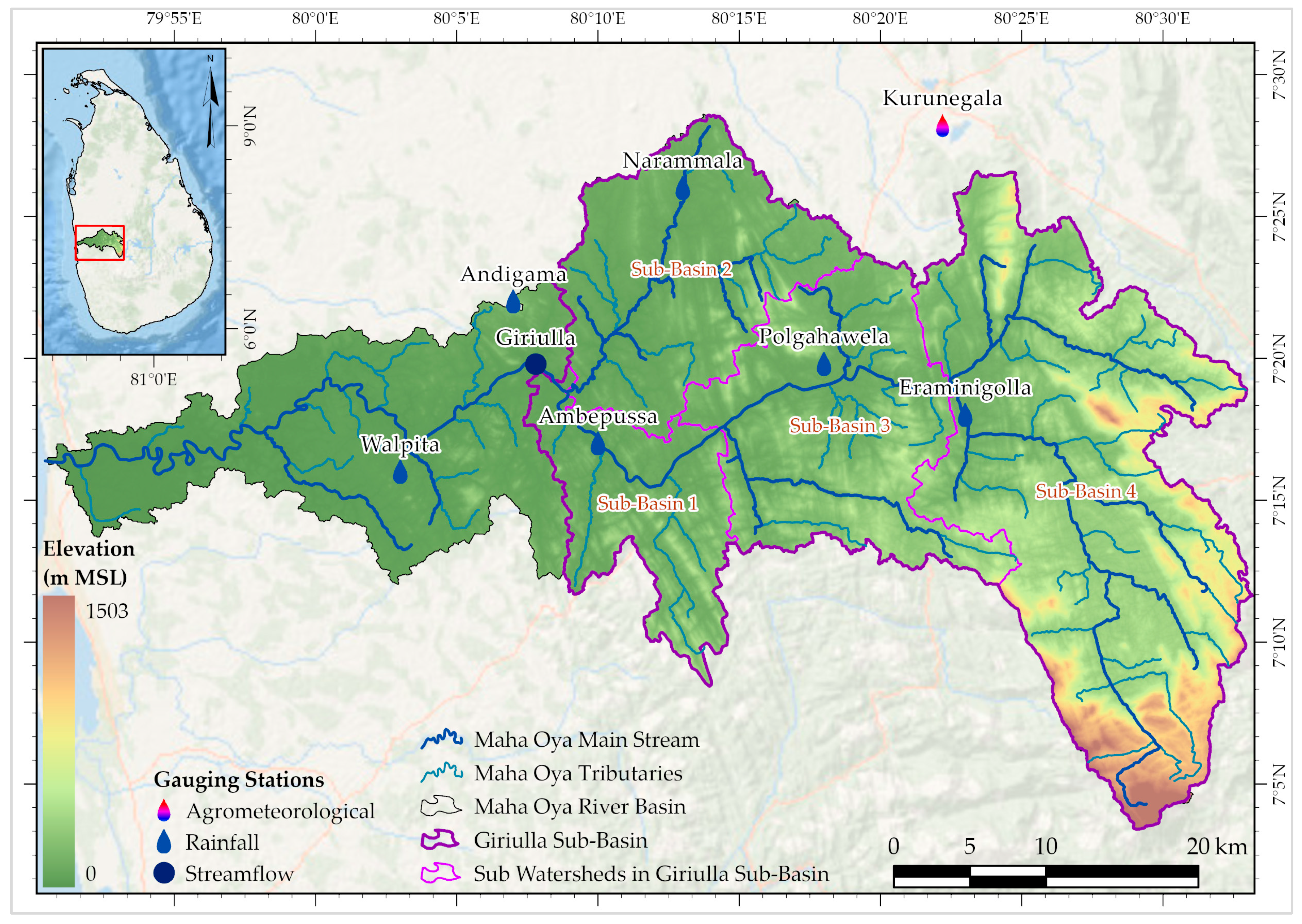
2.1. Study Area

The Maha Oya River Basin is the 11th-largest river basin (with an area of 1410 km2) in Sri Lanka, with its main river (i.e., Maha Oya) stretching 134 km through the country’s wet and intermediate climatic zones (Figure 1). Approximately 75% of the basin lies within the wet zone, while the rest falls within the intermediate zone. The Giriulla sub-basin, located in the upper reaches of the main river basin, covers a total catchment area of 1097 km2, with a 39 km segment of the river flowing through it. This river provides water for over a million people [41]. In this region, the primary economic sector is agriculture, and the main land-use types are forest, vegetation, bare land, settlement, exposed rock, and water bodies. The dominant soil types found in the area are Red–Yellow Podzolic soils, Red–Yellow Podzolic soils and low Humic Gley soils, Redish Brown Latosolic soils, and Red–Yellow Podzolic soils and mountain Regosols soils [42].
Six rain gauge stations cover the full extent of the Giriulla sub-basin. The Thiessen-averaged annual rainfall in the study area is 2144 mm, ranging between 1966 mm and 2358 mm across the six stations during the 2005–2023 period. Seasonal variation in rainfall is significant at all stations (Figure A1). The highest monthly rainfall typically occurs during the Inter-Monsoon 2 period (i.e., October to November), contributing approximately 33% of the annual precipitation. The Southwest Monsoon period accounts for about 36% of the annual rainfall from May to September. In contrast, the Northeast Monsoon period (i.e., from December to February) is considered the dry season because it contributes only 12% of the annual precipitation. The Inter-Monsoon 1 period from March to April also makes a notable contribution of around 19%, with moderately high monthly rainfall. The monthly average maximum temperature peaks in March at 34.8 °C, with an annual average of 32.2 °C for the 2005–2023 period. The monthly average minimum temperature peaks in June at 24.6 °C, with an annual average of 23.2 °C during the same period.

2.2. Hydro-Meteorological and Remote-Sensing Data Collection

The hydro-meteorological data required for developing and testing the Combined Drought Index (CDI) and setting up the hydrological model were obtained from the Meteorological Department (daily rainfall and temperature) and the Irrigation Department (daily river discharge) in Sri Lanka. In addition, the CDI incorporates Land Surface Temperature (LST), the Normalized Difference Vegetation Index (NDVI), and root zone soil moisture (RZSM) from the top 5 cm of the soil column. Therefore, considering the availability of these remote-sensing datasets, the CDI analysis and the application of the hydrological model to assess the spatial variation of drought impacts on streamflow were focused on the period from 2015 to 2023. A digital elevation model (DEM) was used to delineate the watershed boundary and the associated river network. Land-use/land-cover (LULC) data were used to assess the surface imperviousness and describe the land surface characteristics affecting runoff generation. A summary of the spatial and temporal datasets used is provided in Table 2.
Rainfall, temperature, and streamflow datasets used in this study exhibited less than 10% missing values, which falls within the acceptable threshold recommended by the World Meteorological Organization for calculating climatological statistics [43]. Accordingly, the closest station patching method [44] was used for filling in the missing values.

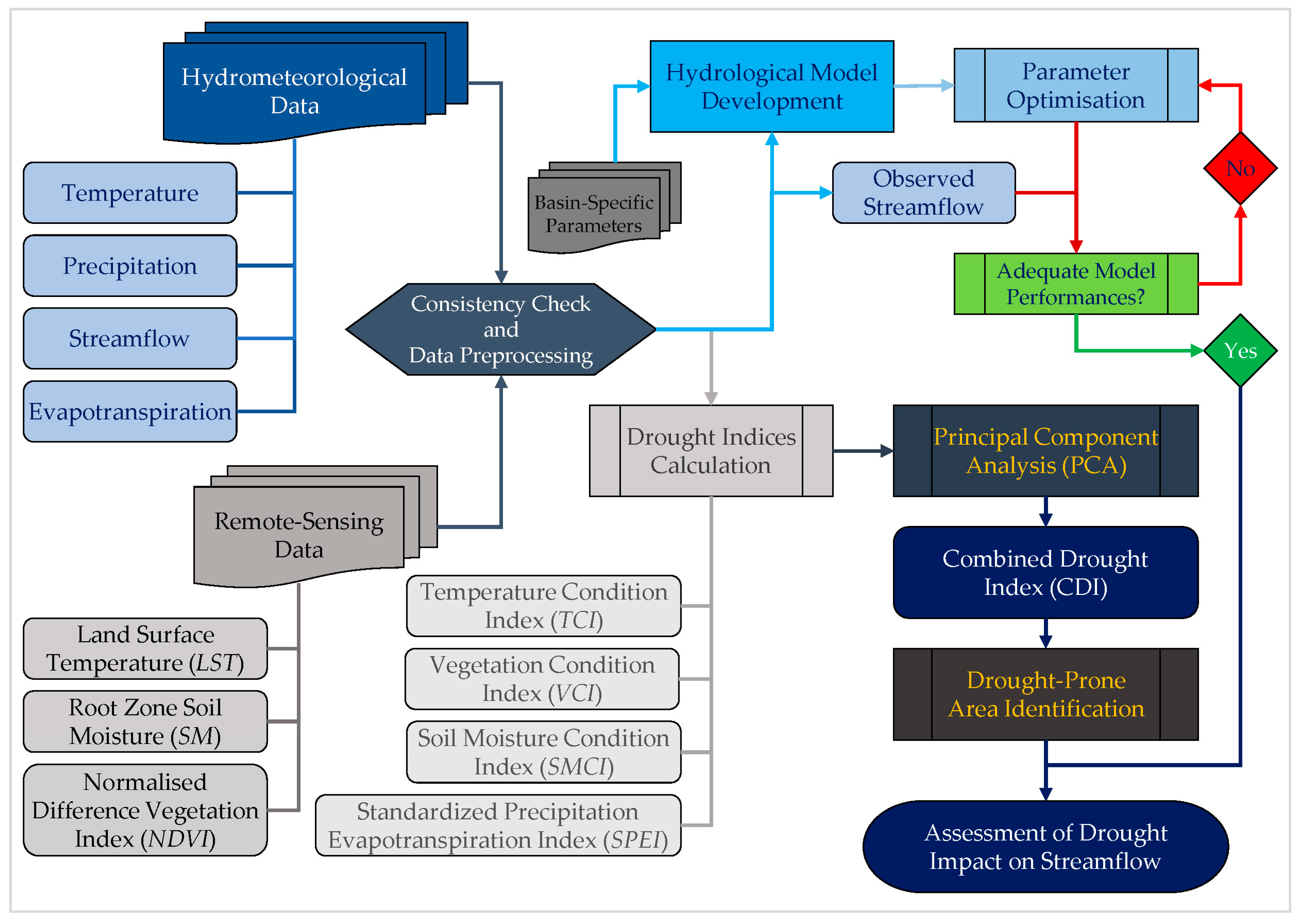
2.3. Development of the Combined Drought Index

Drought is assessed through various indices that represent climatic, land surface, and hydrological conditions. This study developed a combined drought index by integrating four key indicators to capture different drought dimensions. The Standardized Precipitation Evapotranspiration Index (SPEI) represents the climatic aspect by combining precipitation and temperature data. The Temperature Condition Index (TCI) reflects thermal stress using land surface temperature, while the Vegetation Condition Index (VCI) captures vegetation response using NDVI. The Soil Moisture Condition Index (SMCI) accounted for the hydrological component, representing sub-surface water availability. These indices provide a comprehensive understanding of drought impacts across multiple domains.

2.3.1. Standardized Precipitation Evapotranspiration Index (SPEI)

SPEI is a versatile drought indicator that combines precipitation and potential evapotranspiration (PET) to assess drought severity. Unlike the Standardized Precipitation Index (SPI), which only considers precipitation, SPEI incorporates the effects of temperature and evapotranspiration, making it sensitive to water availability and atmospheric demand [45]. SPEI is computed by standardizing the difference between precipitation and PET over a specified period, providing a time-series-based indicator useful for monitoring droughts across various timescales (e.g., SPI-1 for short-term droughts and SPI-12 for long-term droughts). Studies have shown that SPEI is well correlated with drought indices such as SPI but provides a more comprehensive picture by accounting for precipitation deficits and evaporative demand increases [46]. Table A1 shows the drought severity classification of SPEI.

2.3.2. Temperature Condition Index (TCI)

The TCI, derived from thermal infrared remote-sensing data, represents a critical link in the water cycle and heat exchange between the atmosphere, soil, and vegetation. This capability allows TCI to monitor the vegetation growth status and the early stages of drought development [47]. Generally, the TCI derived from MODIS data is considered more effective for short-term drought monitoring. Wei et al. [48] found a positive correlation between MODIS-derived TCI and SPI-3, suggesting its suitability for long-term drought assessments. TCI is calculated as follows:
T C I = L S T m a x , i L S T i , j L S T m a x , i L S T m i n , i
where i = 1, 2, 3, …, 12 denotes for month; j = 1, 2, 3, …, n denotes for year; L S T i , j represents the LST value of the ith month of the jth year; and L S T m a x , i and L S T m i n , i represent the maximum and minimum LST values of the ith month, respectively. Table A2 summarizes the drought severity variation of TCI, which ranges from 0 to 1. Values of 0 and 1 denote extreme drought and wet conditions, respectively.

2.3.3. Vegetation Condition Index (VCI)

The VCI, developed by Kogan et al. [49], is a normalized vegetation indicator designed to improve drought detection by accounting for environmental variability across regions. While NDVI alone reflects vegetation health, its interpretation can be misleading in areas with varying land cover or climate. VCI addresses this limitation by comparing current NDVI values with historical minimum and maximum NDVI values for the same location, thereby capturing vegetation stress relative to typical local conditions [47]. This approach enhances the sensitivity of drought monitoring, especially in diverse ecosystems. VCI is calculated as follows:
V C I = N D V I i , j N D V I m i n , i N D V I m a x , i N D V I m i n , i
where i = 1, 2, 3, …, 12 denotes for month; j = 1, 2, 3, …, n denotes for year; N D V I i , j represents the NDVI value of the ith month of the jth year; and N D V I m a x , i and N D V I m i n , i represent the maximum and minimum NDVI values of the ith month, respectively. According to Table A2, the VCI values range from 0 to 1, denoting extreme drought and wet circumstances, respectively.

2.3.4. Soil Moisture Condition Index (SMCI)

The SMCI is a key drought indicator, directly reflecting soil water/moisture content availability at different depths, making it especially valuable for short-term drought monitoring. SMCI is derived from remote-sensing data, notably from NASA’s Soil Moisture Active Passive (SMAP) satellite. SMAP’s Level-4 (L4) product provides global 3-hourly soil moisture measurements at a 9 km × 9 km spatial resolution, encompassing both surface (0–5 cm depth) and root zone (0–100 cm depth) soil moisture [50]. These measurements are obtained by assimilating SMAP’s L-band brightness temperature observations into a land surface model, offering valuable insights into soil moisture dynamics. SMCI quantifies deviations in current soil moisture levels relative to historical extremes, providing spatially consistent and timely assessments of drought severity. Studies have shown that SMCI correlates well with short-term drought indices like SPI-1, particularly in cultivated and grassland areas, although this relationship may weaken in densely forested regions due to canopy interference [48]. While SMCI may have limited sensitivity to long-term drought trends, it remains essential for capturing rapid changes in surface moisture conditions and enhancing early drought detection. SMCI can be calculated as:
S M C I = S M i , j S M m i n , i S M m a x , i S M m i n , i
where i = 1, 2, 3, …, 12 denotes for month; j = 1, 2, 3, …, n denotes for year; S M i , j represents the SM value of the ith month of the jth year; and S M m a x , i and S M m i n , i represent the maximum and minimum SM values of the ith month, respectively. The SMCI values, presented in Table A2, range from 0 to 1, indicating extreme drought and wet conditions, respectively.

2.3.5. Spatial Dynamics of Drought Parameters

Although Sri Lanka receives substantial annual rainfall, droughts have caused significant disruptions nationwide. One of the most severe droughts in the past 4 decades occurred in 2016, impacting more than 1.8 million people across 20 districts (out of 25), including the Giriulla River Basin [51]. Therefore, as an example, SPEI-1, TCI, VCI, and SMCI were used to examine drought variables’ temporal and spatial dynamics in 2016. Rainfall measurements indicate that precipitation was notably higher in April and May than in June and July (Figure A1). This fluctuation is reflected in the SPEI-1 values, as depicted in Figure 2. The entire basin exhibited higher positive SPEI-1 values in May, indicating wet conditions. TCI was only 0.2 in May but reached 0.6 and 0.95 in June and July, respectively. Correspondingly, VCI values approached 1.0, indicating increased vegetation growth. However, VCI declined to approximately 0.4 during June and July, reflecting reduced vegetation activity. Similarly, the SMCI shows that the soil moisture content is higher in May (0.9). On the other hand, SMCI values decreased to 0.8 and 0.5 in June and July, respectively, indicating less soil moisture availability. The spatial variation of these indices is distinctly observable in the TCI, VCI, and SMCI distributions for April, May, June, and July. In April and May, the downstream regions of the basin consistently exhibited higher VCI values than the upstream areas. Meanwhile, the TCI and SMCI patterns revealed notable differences in surface temperature and soil moisture between the downstream and upstream regions. When comparing April, June, and July, the regional distribution of SPEI-1 suggests that the whole basin had experienced lower SPEI-1 levels. In April, SPEI-1 reached −0.5, suggesting more intense drought conditions than in May. This pattern is also reflected in the TCI, VCI, and SMCI variations. Notably, SMCI was as low as 0.1 in April, whereas it increased to 0.9 by May, indicating a substantial rise in soil moisture content.

2.3.6. Formulating Combined Drought Index (CDI)

A variety of statistical techniques have been applied to formulate Combined Drought Indices (CDIs), including the Analytical Hierarchy Process (AHP) [52], multivariate linear regression [53], and copula-based methods [54]. Among these, Principal Component Analysis (PCA) stands out due to its ability to reduce data redundancy while capturing the underlying variance in multi-index drought datasets, making it particularly effective when reliable in situ data are limited [55,56]. PCA identifies uncorrelated principal components (PCs) that capture key variance patterns by standardizing input data and constructing correlation matrices. The contributions of each index, such as SPEI, TCI, VCI, and SMCI, can then be derived by combining PC loadings with the variance explained by each component [57].
In this study, TCI, VCI, and SMCI were first independently formulated as singular remote-sensing drought indices to formulate the CDI. The 3-hourly Soil Moisture (SM) data were aggregated to a monthly temporal resolution utilizing the arithmetic mean method to establish a temporally consistent dataset. To ensure spatial coherence across variables, the Land Surface Temperature (LST) dataset, which had an initial spatial resolution of 5.6 km, and the Normalized Difference Vegetation Index (NDVI) dataset, which had a spatial resolution of 1 km, were upscaled to a 9 km spatial resolution concurrently using bilinear interpolation. After this upscaling, the TCI, VCI, and SMCI, which represent drought-related fluctuations within their respective domains, were calculated as described in Equations (1)–(3). All input datasets must be consistent with a comparable spatiotemporal framework with a monthly temporal scale and a 9 km spatial resolution to make the CDI formulation process smoother. The Inverse Distance Weighting (IDW) method was employed to interpolate the SPEI-1 (1-month SPEI) values to a gridded 9 km resolution to ensure spatial continuity. The TCI, VCI, and SMCI were normalized and combined to form the CDI, as shown in Equation (4):
C D I i , j = S P E I - 1 i , j × W S P E I ,   i + s t d T C I i , j × W   T C I ,   i + s t d V C I i , j × W V C I ,   i + s t d S M C I i , j × W S M C I ,   i
where CDIi,j, SPEI-1i,j, stdTCIi,j, stdVCIi,j, and stdSMCIi,j represent the CDI, SPEI-1, standardized TCI, standardized VCI, and standardized SMCI of the ith month of the jth year, respectively. Similarly, WSPEI,i, WTCI,i, WVCI,i, and WSMCI,i represent the weight of each index for the ith month.
When developing the CDI, the PCA method was employed to discern the intrinsic structure within the dataset, with SPEI-1, TCI, VCI, and SMCI serving as the primary input variables. For each 9 km × 9 km grid, a covariance matrix was constructed monthly, integrating historical data from 2015 to 2023. These matrices facilitated the derivation of eigenvectors, which explain the relative contributions of each variable, and eigenvalues, which represent the proportion of variance explained by each Principal Component (PC). Each covariance matrix produced four eigenvectors and matching eigenvalues based on the four input variables. The final CDI was constructed using the PC1, which had the highest eigenvalue, thus resulting in the maximum explained variance and ensuring the index captured the most prominent drought-related variables present in the sample. The resultant CDI, characterized by a 9 km × 9 km spatial resolution, was subsequently spatially averaged for validation purposes using standardized streamflow as derived in Equation (5),
s t d S t r e a m f l o w i , j = D i , j μ i σ i
where s t d S t r e a m f l o w i , j , D i , j ,  μ i ,   σ i are the standardized streamflow for the ith month of the jth year, streamflow for the ith month of the jth year, mean of the streamflow of the ith month throughout all years, and standard deviation of the streamflow of the ith month throughout all years, respectively.
The reliability of the CDI was statistically confirmed using the Kolmogorov–Smirnov (KS) test, which examines distributional alignment [58], Pearson’s correlation coefficient, which evaluates linear relationships [31], and Root Mean Square Error (RMSE), which quantifies deviation magnitudes. CDI’s 50%, 20%, 10%, and 5% percentiles were selected as the thresholds for mild, moderate, severe, and extreme drought events, respectively. These classifications are presented in Table A3.

2.4. Hydrological Model Setup, Calibration, and Validation

The Hydrologic Engineering Center, Hydrologic Modelling System (HEC-HMS), is a semi-distributed, physically, and conceptually based hydrological model offering substantial flexibility for streamflow simulation in various geographic regions [59]. A high-resolution 30 m × 30 m Digital Elevation Model (DEM) was used to delineate the catchment, allowing for the accurate extraction of drainage networks, watershed boundaries, and flow accumulation patterns essential for modelling hydrological processes.
The study area was segmented into four sub-basins, and a continuous simulation that includes several methods (Table A4) was undertaken to assess the severity of the spatially varied drought on streamflow. Daily precipitation data were gathered from neighbouring rain gauge stations (viz., Narammala, Ambepussa, Polgahawela, and Eraminigolla for sub-basins 01–04, respectively (Figure 1)), while monthly averaged evapotranspiration data for Kurunegala were taken from the Hydrological Annuals of the Irrigation Department, comprising model calibration/validation and event simulation periods.
Model calibration at the Giriulla gauging station (Figure 1) was performed using daily data from 2003–2005, and validation was conducted with data from 2006–2008. The Nash–Sutcliffe Efficiency (NSE), its logarithmic form (NSElog), and Percent Bias (PBIAS) were chosen as the primary objective functions to evaluate the effectiveness and performance of the model. NSE (Equation (6)) is highly sensitive to peak flows, often prioritizing high-flow accuracy over low-flow representation. On the other hand, NSElog (Equation (7)) enhances sensitivity to low-flow conditions by reducing the influence of high flows through logarithmic transformation, thus offering a more balanced assessment across flow regimes. It is beneficial during dry periods when low-flow accuracy is critical. The PBIAS (Equation (8)) is particularly effective in detecting systematic bias, reflecting the average deviation of simulations from observations. The calibrated parameters used in this study are summarized in Table A4. The calibrated and validated model was later utilized to simulate and evaluate the effects of drought on streamflow during the period from 2016 to 2017.
N S E = 1 i = 1 n Q 0 Q s 2 i = 1 n Q 0 Q ¯ 0 2
N S E l o g = 1 i = 1 n l n Q 0 l n Q s 2 i = 1 n l n Q 0 l n Q ¯ 0 2
P B I A S = i = 1 n Q 0 Q s i = 1 n Q 0
Here, Q 0 and Q s are the observed and simulated streamflow, respectively.

2.5. Evaluation of the Impact of Spatial Drought Variation on Streamflow

The spatially averaged Combined Drought Index (CDI) for each sub-basin was computed, and the streamflow simulations were conducted using the developed HEC-HMS model. First, the relationship between the CDI and specific discharge (i.e., discharge per unit catchment area) was examined for each of the four sub-catchments considered. The relationship between the sub-catchment contribution to total discharge (i.e., the percentage contribution of individual sub-basin flow to the overall flow) and the sub-catchment drought anomaly, defined as the difference between the sub-catchment-averaged CDI and the catchment-averaged CDI, was further investigated. This analysis aimed to evaluate the impact of spatial drought variability on overall streamflow. The evaluation was conducted independently for low flows (represented by the baseflow component during the 2016 and 2017 drought years) and high flows (represented by the direct runoff component). The correlation between the sub-catchment drought anomaly and the sub-catchment contribution to total discharge (%) was demonstrated visually for every sub-basin. The sign and amplitude of these plots’ gradient quantitatively characterize the impact of spatial drought heterogeneity on stream flow dynamics. The overall methodology used in the study is presented in Figure 3.

3. Results

The following sub-sections discuss the relationship between drought parameters and streamflow and the development of the combined drought index. Furthermore, it presents the impacts of spatial variation of drought on stream flow at the sub-basin scale.

3.1. Relationship Between Individual Drought Parameters and Streamflow

The correlation between individual drought indices and standardized streamflow was calculated using Pearson’s correlation coefficient to assess their influence on streamflow between 2015 and 2023. The analysis indicated a significant association between precipitation and streamflow, which showed a strong positive correlation of 0.73 between SPEI-1 and standardized streamflow, implying that enhanced streamflow within the basin directly results from increased precipitation. Similarly, SMCI and normalized streamflow revealed a statistically significant positive association of 0.69, suggesting that higher precipitation levels cause surface runoff to increase, raising soil water content and improving soil moisture conditions as measured by the SMCI. A moderate positive correlation of 0.38 was observed between the Vegetation Condition Index (VCI) and standardized streamflow. This moderate correlation suggests that periods of increased streamflow tend to coincide with improved vegetative conditions, although this relationship is likely driven by shared dependence on precipitation and soil moisture availability rather than a direct influence of streamflow on vegetation. In contrast, the Temperature Condition Index (TCI) exhibited a weak positive correlation of 0.06 with standardized streamflow, indicating a negligible or near-neutral association between temperature conditions and streamflow dynamics in the basin.

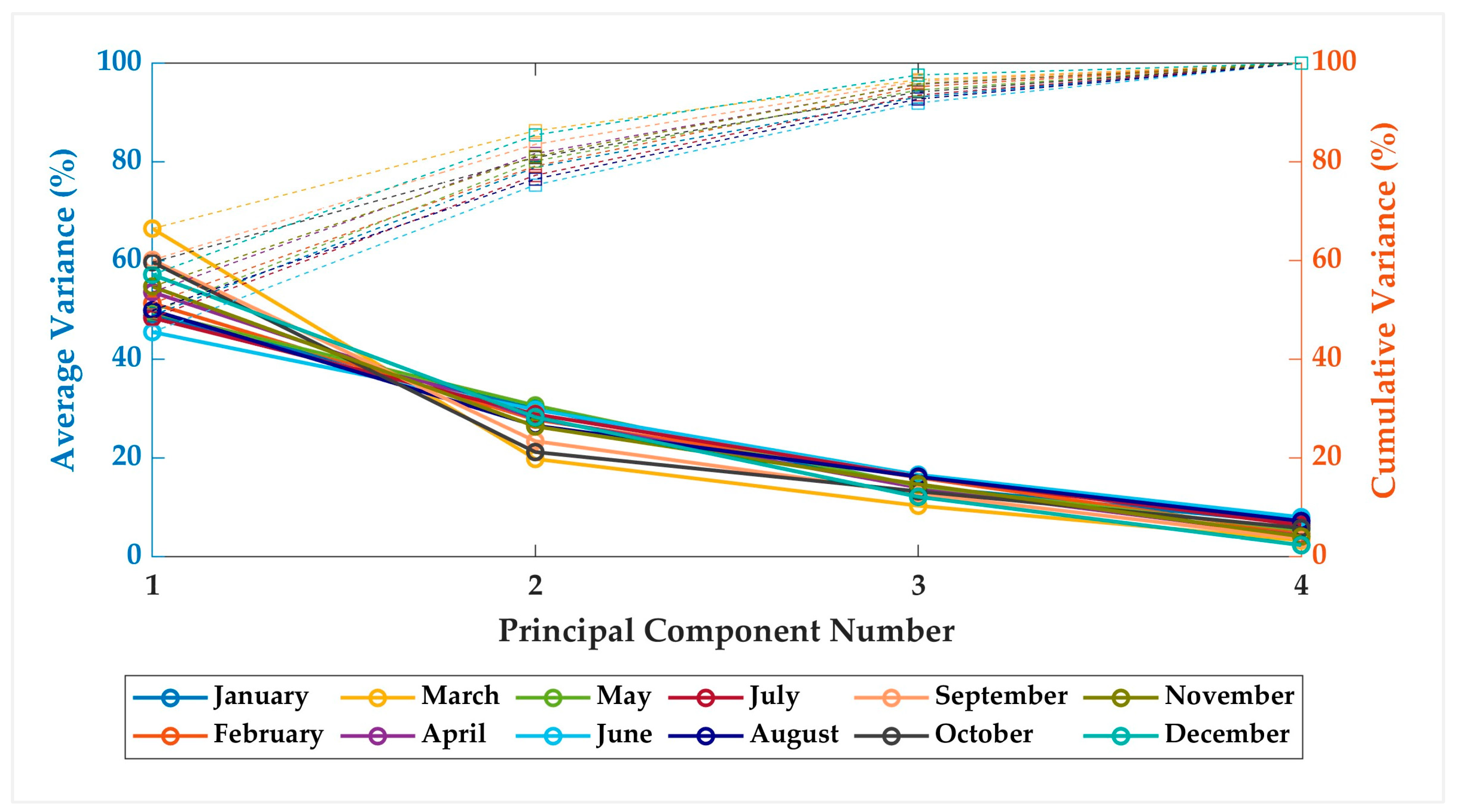
3.2. Principal Component Analysis (PCA)

This analysis used a raster dataset of 21 grids, each containing 12 covariance matrices (i.e., one per month). For each grid, Principal Component Analysis (PCA) was independently performed using monthly data from over nine years (2015–2023). Each covariance matrix was decomposed into four eigenvectors and their corresponding eigenvalues. The eigenvectors represent the contribution (or weight) of each variable, namely the 1-month Standardized Precipitation Evapotranspiration Index (SPEI-1), Temperature Condition Index (TCI), Vegetation Condition Index (VCI), and Soil Moisture Condition Index (SMCI). The eigenvalues indicate the percentage of variance explained by each principal component (PC).
The eigenvector associated with the highest eigenvalue was selected to construct the Combined Drought Index (CDI), as it accounts for the largest proportion of variance and is thus considered the most dominant in describing regional drought patterns. As shown in Table 3, the proportion of variance explained by the leading principal component varied throughout the year, with the highest value observed in March (66.5%) and the lowest in June (45.5%). Figure 4 further illustrates the variance explained by each of the principal components and their cumulative contributions.

3.3. Correlation of the Combined Drought Index (CDI) with Component Indices

The CDI produced strong Pearson’s correlation coefficients with SMCI (r = 0.78) and SPEI (r = 0.73), indicating its high sensitivity to soil moisture and climatic variations. These relationships highlight the critical influence of precipitation on both indices—SPEI reflects reduced drought stress with increased rainfall, while SMCI captures improved root zone moisture conditions. The VCI demonstrated a moderate correlation (r = 0.62) with the CDI, suggesting that better hydrological conditions positively affect vegetation health. In contrast, the TCI exhibited only a weak correlation (r = 0.29), indicating a limited influence of temperature on the composite index. This suggests that while temperature may contribute to drought conditions, precipitation and soil moisture are more decisive factors, especially in water-limited regions. Overall, the correlation analysis underscores the importance of integrating multiple indicators, particularly those related to precipitation and soil moisture, for a comprehensive and robust drought assessment framework.

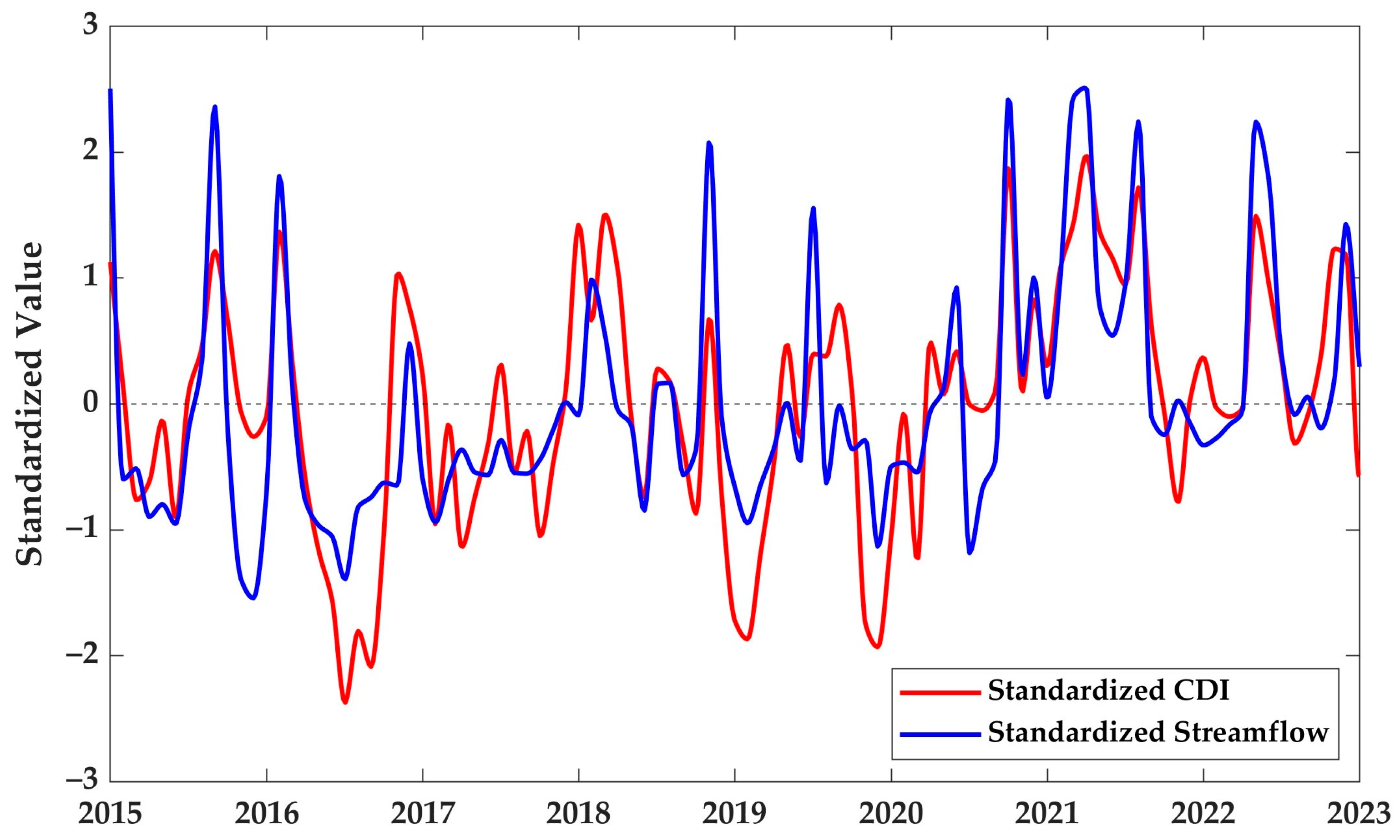
3.4. Combined Drought Index (CDI) and Validation with Streamflow

The temporal and spatial variations of the CDI are illustrated in Figure 5. The basin generally receives higher rainfall during the Southwest Monsoon (June to September) and the First Inter-Monsoon (October to November) (Figure A1). However, during the 2016 drought, a significant portion of the basin was identified as drought-prone from July to November, which coincided with these two monsoon periods.
A comparison between Figure 2 and Figure 5 highlights the influence of individual drought indices from April to July 2016. During this period, particularly in May, increased precipitation led to higher values in the SPEI-1, along with higher SMCI values and improved VCI readings. This combination of favourable conditions is reflected in Figure 5, where a substantial portion of the basin exhibited wet conditions in May. However, by July, the impact of decreasing VCI and SPEI-1 became evident, resulting in widespread moderate-to-severe drought conditions. Furthermore, severe drought persisted across most of the basin in September, October, and December of 2016, classifying 2016 as a drought year.
The spatially averaged CDI values for the Giriulla sub-basin were extracted and standardized using the CDI’s monthly mean and standard deviation. This standardization enabled a direct comparison between the CDI and standardized streamflow data over nine years. A Pearson correlation coefficient of 0.74 between the standardized CDI and streamflow indicates a strong positive relationship. This consistent correlation shows that a decline in the CDI (toward negative values) corresponds to reduced streamflow, reflecting drier conditions, whereas an increase in the CDI (toward positive values) is associated with higher streamflow and wetter conditions.
Figure 6 illustrates the temporal variation of standardized streamflow and CDI. The Root Mean Square Error (RMSE) of 0.68 indicates a relatively small difference. Furthermore, a Kolmogorov–Smirnov (KS) test was conducted to assess whether the two distributions originated from the same underlying population. The null hypothesis could not be rejected at the 95% confidence level, suggesting no statistically significant difference between them. Together, these three validation metrics (viz., correlation coefficient, RMSE, and KS test) support the robustness and reliability of the proposed CDI in capturing the temporal dynamics of drought.

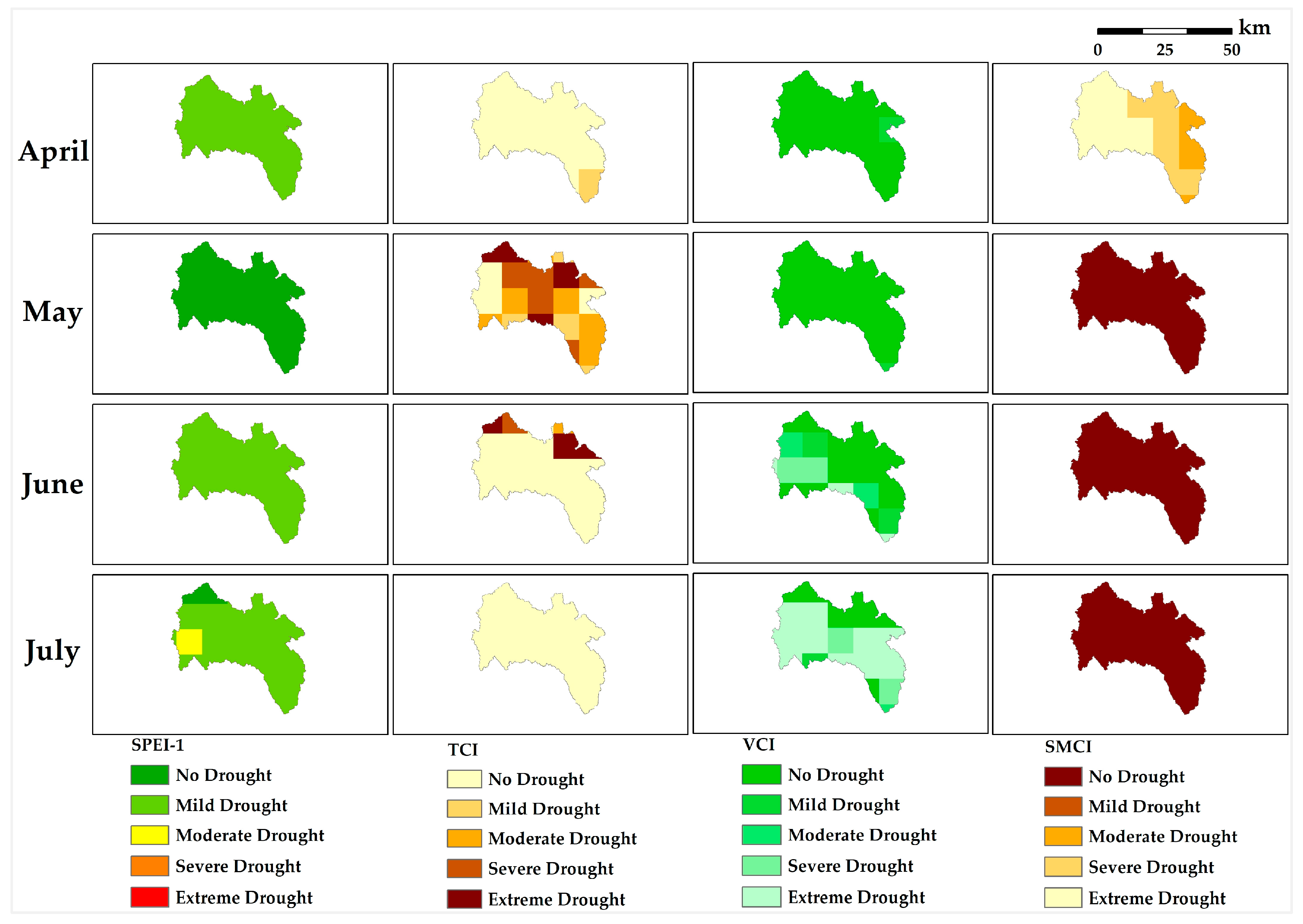
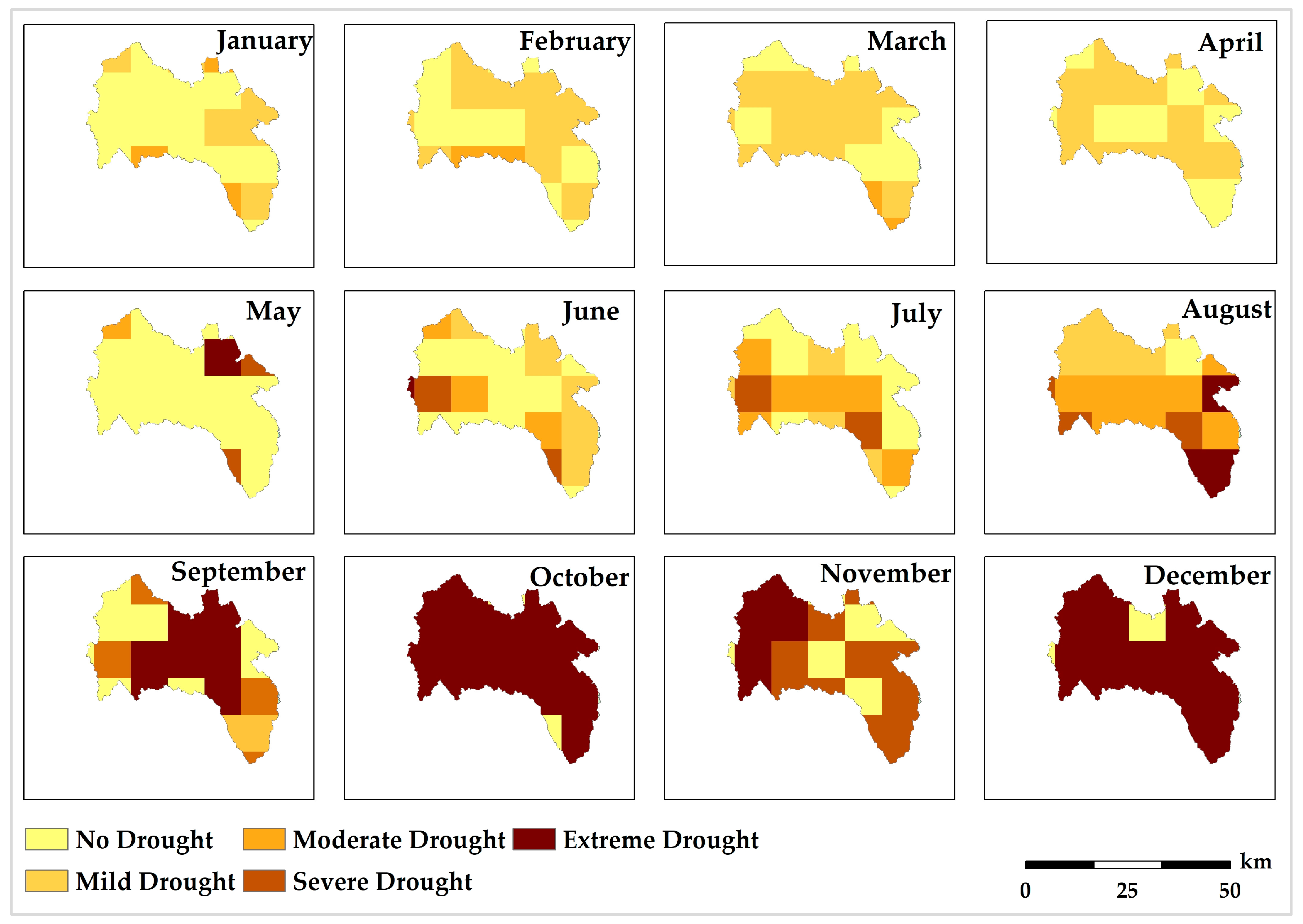
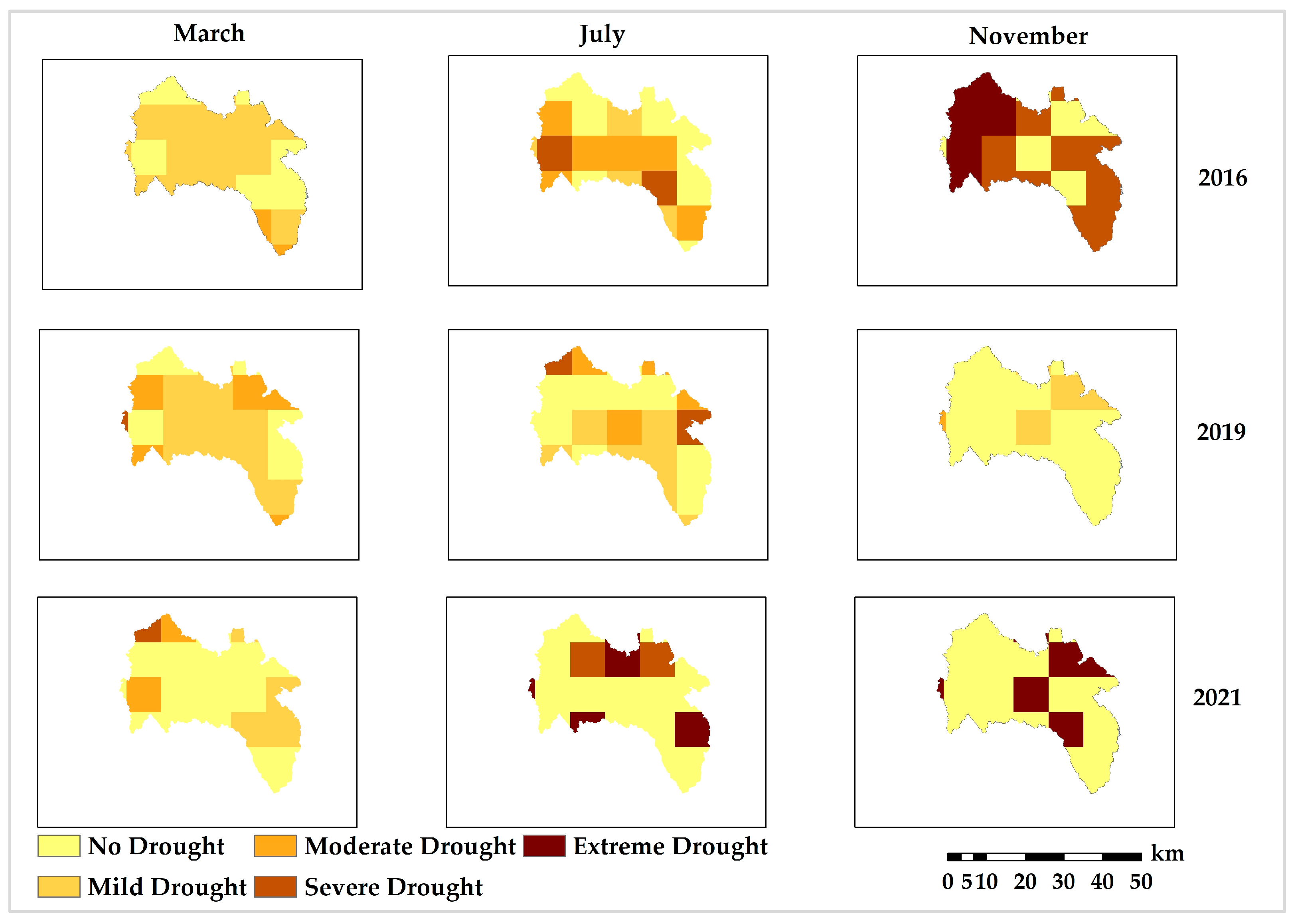
3.5. Spatial and Temporal Dynamics of Drought

During the study period (2015–2023), the region experienced two major extreme events, i.e., the 2016 drought [51] and the 2021 flood [60], which were effectively captured by the developed CDI (Figure 6). The CDI identified these individual drought and flood events and revealed intra-annual transitions between dry and wet conditions. The temporal and spatial analysis in Figure 7 shows that a significant portion of the basin experienced extreme dry conditions in November 2016. In contrast, predominantly wet conditions were observed in March 2021 (Figure 7), which transitioned to dry conditions by November 2021, with severe drought persisting in upstream regions. Additionally, minor drought conditions were evident in March 2016 and 2019, corresponding with typical seasonal precipitation deficits. These findings underscore the novel CDI’s effectiveness in capturing dynamic hydrological variability, which is crucial for informed water resources management.

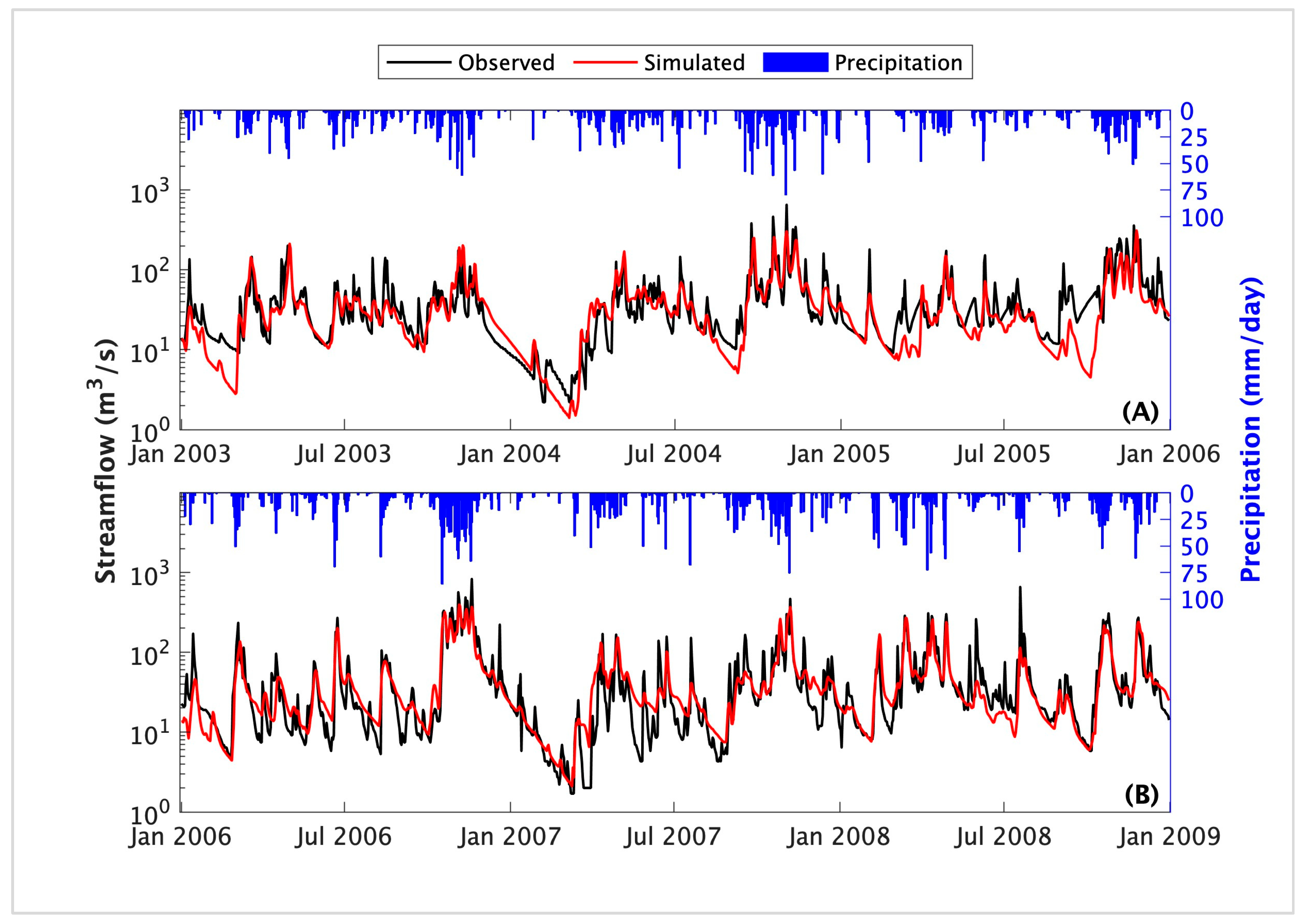
3.6. Hydrological Model Performance and Streamflow Simulation

A continuous HEC-HMS model was developed to further investigate the impact of spatial drought variability on stream flow. The model was calibrated and validated over 2003–2005 and 2006–2008, respectively. Key performance indicators, Nash–Sutcliffe Efficiency (NSE), its logarithmic form (NSElog), and Percent Bias (PBIAS), were used through a combination of automated and manual calibration, ensuring reproducibility of observed data at the Giriulla Gauging station (Figure 8 and Figure A1).
Low-flow performance was evaluated using NSElog, which yielded values of 0.61 and 0.81 during calibration and validation periods, respectively, indicating the model’s effectiveness in simulating dry conditions. The conventional NSE, which is more sensitive to peak flows, yielded 0.60 and 0.74 for calibration and validation, respectively, demonstrating reliable high-flow representation. PBIAS values of 15.5% (calibration) and 11.1% (validation) confirmed the model’s accuracy, indicating minimal bias across both periods. Table 4 summarizes these performance matrices for calibration and validation periods.

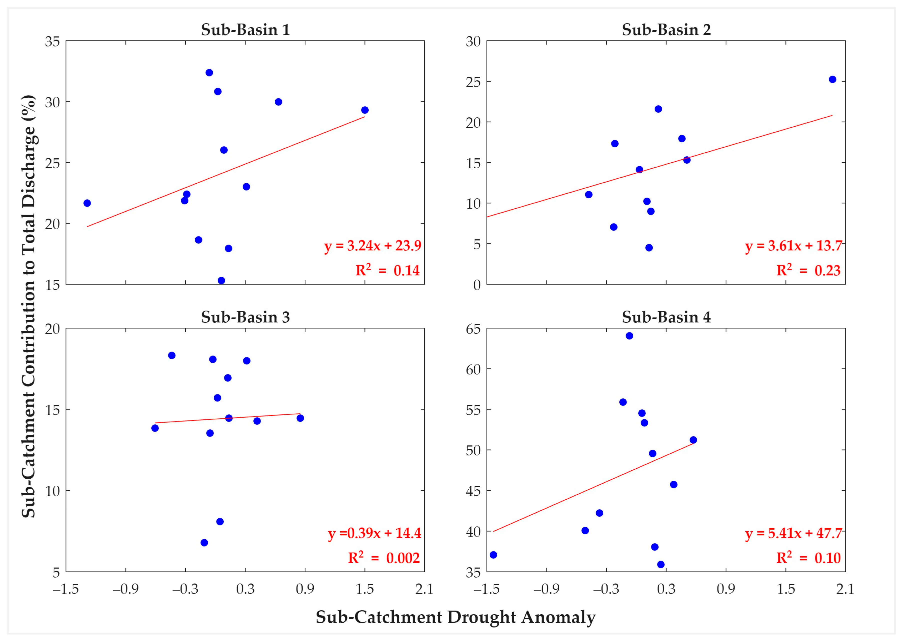
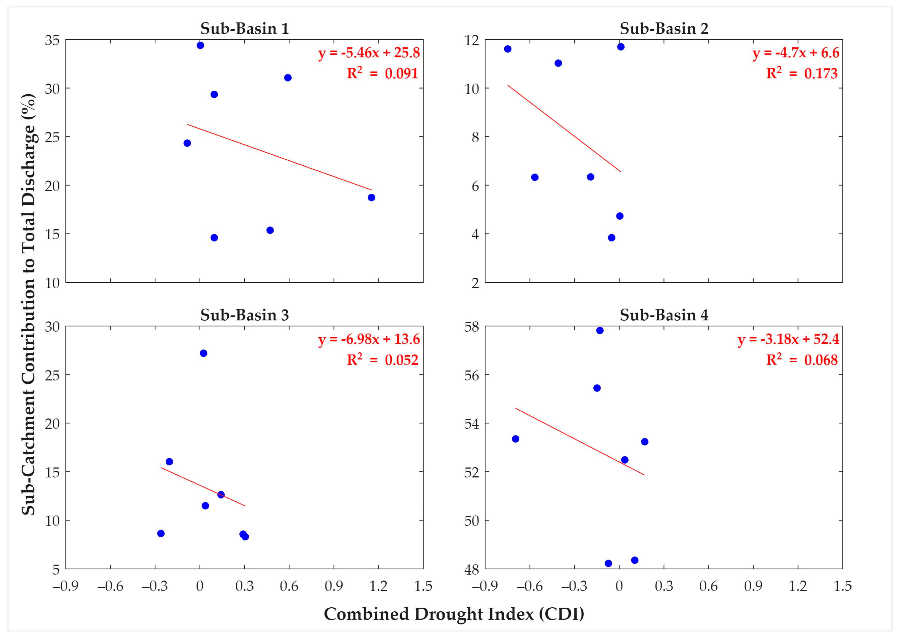
3.7. Impact of Spatial Drought Variation on Streamflow

Figure 9 shows the variation of specific discharge (discharge per unit catchment area, in m3/s/km2) with the Combined Drought Index (CDI) averaged over each sub-catchment. Across all four sub-catchments, specific discharge declines markedly with increasing drought severity. Upper catchments exhibit greater sensitivity to drought conditions than lower catchments. Specifically, sub-catchment 4 (representing the upper region of the river basin) has an exponential coefficient of 0.66, while sub-catchment 1 (a downstream region) shows a lower coefficient of 0.38. This low correlation indicates that the upper catchment’s specific discharge is approximately 75% more sensitive to drought severity than the lower catchment, highlighting the stronger hydrological response of upstream areas to drought variations.
Figure 10 and Figure 11 illustrate the relationship between the sub-catchment contribution to total discharge (%) and their drought anomaly (the difference between the sub-catchment-average CDI and the catchment-average CDI), estimated for the direct runoff component and baseflow component during drought years 2016 and 2017, respectively. Positive drought anomaly values indicate that the sub-catchment is wetter than the overall catchment average, while negative values indicate that the sub-catchment is drier than average. In Figure 10 (direct runoffs), most sub-catchments show a positive relationship, implying that wetter sub-catchments contribute more to total discharge during high-flow events. In contrast, Figure 11 (baseflows) shows negative relationships, suggesting that some sub-catchments can sustain or even increase their relative contribution to baseflow, even under drier conditions.
Notably, sub-catchments with longer flow paths and larger catchment sizes (e.g., sub-catchment 4) show less sensitivity in baseflow contribution to drought anomaly (i.e., a smaller gradient magnitude in trendlines), which may reflect delayed or buffered baseflow responses due to longer travel times or larger groundwater storage systems associated with larger catchment areas. In contrast, sub-catchments with shorter flow paths (e.g., sub-catchments 1 and 2) exhibit greater sensitivity, indicating faster and more direct baseflow responses to local drought conditions. These findings highlight the importance of considering spatial differences in drought sensitivity and flow response when managing water resources. In particular, upstream areas with delayed baseflow responses could serve as critical buffers during drought periods, emphasizing the need for targeted groundwater conservation and drought resilience strategies across the catchment.

4. Discussion

Single-variable drought indices such as SPI, NDVI, or SSI are limited in their ability to capture the full complexity of droughts, particularly in regions with limited ground-based data and heterogeneous land cover. Remote sensing offers valuable spatial coverage and consistency, making it suitable for large and data-scarce river basins. Combined Drought Indices (CDIs), which integrate multiple drought indicators, provide a more holistic representation of drought conditions by simultaneously capturing climatic, hydrological, and ecological stressors. Kulkarni et al. [61] showed that a CDI combining meteorological and agricultural anomalies outperformed single indices in identifying socio-economic droughts, successfully detecting 1885 out of 2142 events, which is more than SPI, NDVI, or SSI are individually capable of. Similarly, Bajracharya et al. [31] demonstrated that a CDI incorporating LST, NDVI, snow cover, and precipitation strongly correlated (r = 0.78) with standardized streamflow in the Narayani River Basin, highlighting its reliability in monitoring spatial drought variation. This study adapts and modifies the CDI framework by replacing the snow cover component with root-zone soil moisture derived from SMAP L4 data, making it more suitable for rain-fed catchments where soil moisture plays a critical role in drought dynamics. These findings emphasize the importance of using combined indices for robust drought assessment, particularly in large tropical basins like the Maha Oya.
The spatial variability of droughts across river basins is well-documented, with several studies confirming that upstream and downstream regions respond differently to drought conditions. For instance, Hendawitharana et al. [62] found that in the Kirindi Oya Basin, Sri Lanka, drought characteristics varied significantly between the upper and lower sub-basins due to differing climatic zones and land cover, underscoring the importance of sub-basin scale assessments. Similarly, Wu et al. [63], in a remote-sensing-based analysis of the Koshi River Basin, China, observed that upstream areas experienced more severe droughts in certain seasons than downstream regions, particularly due to the spatial differences in vegetation, precipitation, and temperature. These findings are consistent with our study in the Giriulla sub-basin, where the upstream sub-catchments demonstrated greater sensitivity to drought conditions, with sharper reductions in specific discharge. These findings support the need for spatially explicit drought indices like the Combined Drought Index (CDI) used in our analysis, which captures such heterogeneity. Moreover, Dahlmann et al. [64] highlighted upstream–downstream asymmetries in drought impacts across major European river basins, noting that although downstream regions often report more impacts, the drivers and hydrological responses vary spatially, further reinforcing the need for detailed sub-basin evaluations in both scientific assessments and water management planning.
The impact of drought varies significantly between high- and low-flow conditions, and this variation is closely linked to spatial differences in catchment characteristics. A global analysis by Liu et al. [65] found that wetter regions tend to contribute more to streamflow during high-flow periods, while their resilience during drought-induced low-flows depends on climate and catchment-specific factors such as storage capacity and evapotranspiration. Supporting these findings, Fernando et al. [66] showed that certain sub-catchments in Sri Lanka’s Kalu River Basin sustained baseflows more effectively during droughts due to favourable catchment characteristics such as soil retention and land cover. These studies reinforce our observation in the Giriulla sub-basin, where wetter sub-catchments contributed more during high-flow events, while resilience during low-flow periods varied depending on geomorphological and hydrological features, thus underscoring the importance of integrating sub-catchment characteristics into drought assessments and flow simulations to improve water resource planning and drought resilience strategies.

5. Conclusions

This study tested a novel methodology that integrates a Combined Drought Index (CDI) with a semi-distributed hydrological model to assess the spatio-temporal variability of drought impacts on stream flow, using the Giriulla sub-basin of the Maha Oya River Basin in Sri Lanka as a case study. The CDI, formulated by merging standardized remote-sensing-based indicators (viz., SPEI, TCI, VCI, and SMCI) using Principal Component Analysis (PCA), effectively captured both temporal and spatial drought patterns. Validation against standardized streamflow demonstrated a strong positive correlation (Pearson correlation coefficient of 0.74), confirming the CDI’s ability to reflect hydrological drought conditions. Spatial analyses revealed that upper sub-catchments exhibited greater sensitivity to drought severity than downstream areas, with specific discharge reducing more sharply in response to drier conditions.
During high-flow periods dominated by direct runoff, wetter sub-catchments contributed proportionally more to total discharge, indicating a generally positive relationship between spatial drought anomalies and high-flow contributions. In contrast, during low-flow periods primarily sustained by baseflow, some drier sub-catchments demonstrated relative resilience by maintaining streamflow contributions despite drier conditions, though with variable sensitivity across the basin. These contrasting patterns underscore the spatial heterogeneity and nonlinear nature of hydrological responses to drought.
It is important to note that the Combined Drought Index (CDI), developed using short-term indicators such as SPEI-1, TCI, VCI, and SMCI at a monthly temporal scale, primarily reflects meteorological drought conditions and their immediate impact on streamflow. While this approach captures short-term variability, it does not explicitly account for the delayed onset and prolonged duration associated with hydrological or agricultural droughts. Future work could extend this framework by incorporating longer-term indicators (e.g., SPEI-3, groundwater anomalies) to address multi-scale drought propagation and improve the representation of spatiotemporal heterogeneity.
While Figure 10 and Figure 11 do not exhibit a strong statistical fit due to the system’s complexities, they reveal important emergent trends. The intent is not to produce predictive models but to illustrate how spatiotemporal variability in drought severity influences streamflow behaviour. The integration of remote sensing and hydrological modelling in this study provides a valuable framework for understanding these dynamics, supporting adaptive water resource management and drought mitigation planning under future climate uncertainties.
In this study, important elements, including groundwater availability, ecological reactions, and socioeconomic situations, were not included in the development of the CDI, which was based solely on climatic and land surface indicators (SPEI-1, TCI, VCI, and SMCI). Furthermore, bias adjustment was not conducted during soil moisture (SM) data processing since ground-observed SM data were not readily available. However, this omission is not likely to have a significant effect on the results because the study focuses on capturing spatial variability rather than absolute precision. In developing CDI, PCA may have ignored nonlinear interactions between variables, thus potentially leaving out important information because of the assumed linear correlations. Furthermore, satellite-based inputs like LST, NDVI, and SM may be impacted by resolution limitations and data gaps, especially in areas prone to excessive cloud cover or extensive vegetation. Since those inputs are critical in deriving the CDI, their gaps or limitations in resolution may considerably impact the accuracy of the CDI. For catchments with limited/low streamflow observations, the CDI’s transferability and usefulness are increased by its incorporation into an open-source hydrological model (HEC-HMS).
Furthermore, because the available hydro-meteorological data had substantial inconsistencies, this study’s calibration and validation periods were forced to be shortened when developing the HEC-HMS model. Due to this forced restriction, the model’s performance might not accurately reflect the dynamics of long-term catchment flow, underscoring the necessity of additional validation to evaluate the model’s robustness using larger datasets. Additionally, the analysis period for drought assessment was limited to 2015–2023, primarily due to the availability of key remote-sensing products such as the SMAP L4 Root Zone Soil Moisture data, which have only been available since March 2015. While a longer data record would have provided more profound insights into drought variability, the selected timeframe was sufficient to meet the study’s primary objective, establishing relationships between river discharge and key drought indicators. In addition, although the framework was applied only to the Giriulla sub-basin of the Maha Oya River Basin, this area was specifically chosen for its representative characteristics, including diverse land use, topographic variation, and hydrological response, which make it well-suited for pilot-scale validation. Applying the framework to broader spatial extents in future studies would further enhance its generalizability and validity. Despite these limitations, this study shows strong potential for broader applications. The study relies on freely available remote-sensing datasets and minimal site-specific information, making it generically applicable, particularly in data-scarce regions. Furthermore, future studies should focus on overcoming the above-mentioned constraints while adding climate-change projections for future drought assessments, real-time forecasting, and other drought-relevant indicators, including socio-economic stressors and groundwater details, to increase the framework’s operational utility and comprehensiveness.

Author Contributions

Conceptualization, A.S. and L.G.; methodology, A.S. and L.G.; software, A.S. and L.G.; validation, A.S., L.G. and J.S.; formal analysis, A.S.; investigation, A.S.; resources, L.G. and L.R.; data curation, A.S.; writing—original draft preparation, A.S.; writing—review and editing, A.S., L.G., J.B., J.S. and L.R.; visualization, A.S. and J.B.; supervision, L.G. and J.B.; project administration, L.G. and L.R. All authors have read and agreed to the published version of the manuscript.

Funding

This research received no external funding.

Data Availability Statement

The raw data supporting the findings of this study are available from the authors upon reasonable request. Researchers are encouraged to copy all data requests to umcsawm.research@gmail.com to facilitate prompt processing, monitoring, and administrative record-keeping.

Acknowledgments

The authors gratefully acknowledge the Irrigation Department and the Department of Meteorology, Sri Lanka, for their invaluable support in providing the essential datasets used in this research. Sincere thanks are also extended to the UNESCO-Madanjeet Singh Centre for South Asia Water Management (UMCSAWM) at the University of Moratuwa for their generous support throughout the study.

Conflicts of Interest

The authors declare no conflicts of interest.

Appendix A

Figure A1. Intra-annual rainfall variability within the study area over the 2005–2023 period. The boxes are limited to the 25th and 75th percentiles, and the horizontal line shows the median (i.e., 50th percentile) value of the monthly data sets. Whiskers are extended to 1.5 times inter-quartile range (i.e., range between 25th and 75th percentiles) to the top and bottom of the boxes.
Hydrology 12 00142 g0a1
Table A1. Drought classification of SPEI.
Drought ClassesRange
Extreme Drought≤−2
Severe Drought−2 to −1.5
Moderate Drought−1.5 to −1
Mild Drought−1 to 0
No Drought0 to 3
Table A2. Drought classification of TCI, VCI, and SMCI.
Drought ClassesRange
Extreme Drought<0.1
Severe Drought0.1–0.2
Moderate Drought0.2–0.3
Mild Drought0.3–0.4
No Drought>0.4
Table A3. Drought classification based on CDI.
Drought ClassesRange
Extreme DroughtCDI ≤ −1.7
Severe Drought−1.3 ≤ CDI <−1.7
Moderate Drought−0.8 ≤ CDI < −1.3
Mild Drought0 ≤ CDI < −0.8
No DroughtCDI > 0
Table A4. Utilized methods in HEC-HMS model setup and parameter ranges.
CriteriaParameterSub-Basin 01Sub-Basin 02Sub-Basin 03Sub-Basin 04
Canopy—Simple canopyInitial Storage (%)0.270.270.102.26
Max Storage (mm)551010
Crop Coefficient0.640.501.491.49
Surface—Simple SurfaceInitial Storage (%)1.71.32.93.3
Max Storage (mm)8101114
Loss—Soil Moisture AccountingSoil (%)4.65.71.25.0
Groundwater 1 (%)3.15.05.34.1
Groundwater 2 (%)5.13.23.14.1
Maximum Infiltration (mm/h)910108
Impervious (%)6666
Soil Storage (mm)102120142105
Tension Storage (mm)25364451
Soil Percolation (mm/h)5420.5
Groundwater 1 Storage (mm)1541515251
Groundwater 1 Percolation (mm/h)2.92.91.80.4
GW1 Coefficient (h)5183117207
Groundwater 2 Storage (mm)300.76300.26300.94300
Groundwater 2 Percolation (mm/h)1.01.41.80.3
GW2 Coefficient (h)155162277299
Transform—SCS Unit HydrographLag Time (min)166150118158
Base flow—Linear ReservoirGW 1 Initial (m3/s)1.72.01.72.0
GW 1 Fraction0.50.50.50.5
GW 1 Reservoirs2222
GW 2 Initial (m3/s)1.51.22.01.4
GW 2 Fraction0.30.30.30.3
GW 2 Reservoirs1111
Routing—MuskingumMuskingum K (h)15.422.916.2
Muskingum X0.200.270.47
Note: The texts in bold are the hydrological processes considered, followed by the selected simulation method in HEC-HMS model setup.

References

  1. World Meteorological Organization. Drought Monitoring and Early Warning: Concepts, Progress and Future Challenges Weather and Climate Information for Sustainable Agricultural Development; World Meteorological Organization: Geneva, Switzerland, 2006. [Google Scholar]
  2. World Meteorological Organization. Weather-Related Disasters Increase over Past 50 Years, Causing More Damage but Fewer Deaths. Available online: https://wmo.int/news/media-centre/weather-related-disasters-increase-over-past-50-years-causing-more-damage-fewer-deaths (accessed on 26 March 2025).
  3. Food and Agriculture Organization of the United Nations. Agriculture on the Proving Grounds: Damage and Loss. Available online: https://www.fao.org/interactive/disasters-in-agriculture/en/ (accessed on 16 April 2025).
  4. Food and Agriculture Organization of the United Nations. Sri Lanka’s Food Production Hit by Extreme Drought Followed by Floods|FAO in Sri Lanka|Food and Agriculture Organization of the United Nations. Available online: https://www.fao.org/srilanka/news/detail-events/en/c/897464/ (accessed on 24 March 2025).
  5. Asian Development Bank. Sri Lanka Climate Risk Country Profile; Asian Development Bank: Mandaluyong City, Philippines, 2020. [Google Scholar]
  6. Naumann, G.; Alfieri, L.; Wyser, K.; Mentaschi, L.; Betts, R.A.; Carrao, H.; Spinoni, J.; Vogt, J.; Feyen, L. Global Changes in Drought Conditions Under Different Levels of Warming. Geophys. Res. Lett. 2018, 45, 3285–3296. [Google Scholar] [CrossRef]
  7. World Health Organization. Drought. Available online: https://www.who.int/health-topics/drought#tab=tab_1 (accessed on 26 April 2025).
  8. Zaveri, E.D.; Damania, R.; Engle, N. Droughts and Deficits: The Global Impact of Droughts on Economic Growth; Policy Research Working Paper; Water Global Practice, The World Bank: Washington, DC, USA, 2023. [Google Scholar]
  9. Jing, F.; Baisha, W.; Cheng, Z.; Qing, W. The Recognition of Drought and Its Driving Mechanism Based on “Natural-Artificial” Dual Water Cycle. Procedia Eng. 2012, 28, 580–585. [Google Scholar] [CrossRef]
  10. Ndayiragije, J.M.; Li, F. Effectiveness of Drought Indices in the Assessment of Different Types of Droughts, Managing and Mitigating Their Effects. Climate 2022, 10, 125. [Google Scholar] [CrossRef]
  11. Cavus, Y.; Aksoy, H. Critical Drought Severity/Intensity-Duration-Frequency Curves Based on Precipitation Deficit. J. Hydrol. 2020, 584, 124312. [Google Scholar] [CrossRef]
  12. Hong, S.; Deng, H.; Zheng, Z.; Deng, Y.; Chen, X.; Gao, L.; Chen, Y.; Liu, M. The Influence of Variations in Actual Evapotranspiration on Drought in China’s Southeast River Basin. Sci. Rep. 2023, 13, 21336. [Google Scholar] [CrossRef]
  13. Mishra, V.; Aadhar, S.; Asoka, A.; Pai, S.; Kumar, R. On the Frequency of the 2015 Monsoon Season Drought in the Indo-Gangetic Plain. Geophys. Res. Lett. 2016, 43, 12,102–12,112. [Google Scholar] [CrossRef]
  14. Guhathakurta, P.; Rajeevan, M. Trends in the Rainfall Pattern over India. Int. J. Climatol. 2008, 28, 1453–1469. [Google Scholar] [CrossRef]
  15. Chen, Y.; Teo, F.Y.; Wong, S.Y.; Chan, A.; Weng, C.; Falconer, R.A. Monsoonal Extreme Rainfall in Southeast Asia: A Review. Water 2024, 17, 5. [Google Scholar] [CrossRef]
  16. Seneviratne, S.I.; Zhang, X.; Adnan, M.; Badi, W.; Dereczynski, C.; Di Luca, A.; Ghosh, S.; Iskandar, I.; Kossin, J.; Lewis, S.; et al. Weather and Climate Extreme Events in a Changing Climate. In Climate Change 2021—The Physical Science Basis; Masson-Delmotte, V., Zhai, P., Pirani, A., Connors, S.L., Péan, C., Berger, S., Caud, N., Chen, Y., Goldfarb, L., Gomis, M.I., et al., Eds.; Cambridge University Press: Cambridge, UK; New York, NY, USA, 2021; pp. 1513–1766. [Google Scholar]
  17. Martínez-Sifuentes, A.R.; Trucíos-Caciano, R.; Rodríguez-Moreno, V.M.; Villanueva-Díaz, J.; Estrada-Ávalos, J. The Impact of Climate Change on Evapotranspiration and Flow in a Major Basin in Northern Mexico. Sustainability 2023, 15, 847. [Google Scholar] [CrossRef]
  18. Doblas-Reyes, F.J.; Sorensson, A.A.; Almazroui, M.; Dosio, A.; Gutowski, W.J.; Haarsma, R.; Hamdi, R.; Hewitson, B.; Kwon, W.-T.; Lamptey, B.L.; et al. Linking Global to Regional Climate Change. In Climate Change 2021: The Physical Science Basis; Masson-Delmotte, V., Zhai, P., Pirani, A., Connors, S.L., Péan, C., Berger, S., Caud, N., Chen, Y., Goldfarb, L., Gomis, M.I., et al., Eds.; Cambridge University Press: Cambridge, UK, 2021. [Google Scholar]
  19. Mishra, V.; Kumar, R.; Shah, H.L.; Samaniego, L.; Eisner, S.; Yang, T. Multimodel Assessment of Sensitivity and Uncertainty of Evapotranspiration and a Proxy for Available Water Resources under Climate Change. Clim. Change 2017, 141, 451–465. [Google Scholar] [CrossRef]
  20. Sanogo, N.D.M.; Dayamba, S.D.; Renaud, F.G.; Feurer, M. From Wooded Savannah to Farmland and Settlement: Population Growth, Drought, Energy Needs and Cotton Price Incentives Driving Changes in Wacoro, Mali. Land 2022, 11, 2117. [Google Scholar] [CrossRef]
  21. Liang, W.; Zhang, W.; Jin, Z.; Yan, J.; Lü, Y.; Li, S.; Yu, Q. Rapid Urbanization and Agricultural Intensification Increase Regional Evaporative Water Consumption of the Loess Plateau. J. Geophys. Res. Atmos. 2020, 125, e2020JD033380. [Google Scholar] [CrossRef]
  22. Eyring, V.; Gillett, N.P.; Achuta Rao, K.M.; Barimalala, R.; Barreiro Parrillo, M.; Bellouin, N.; Cassou, C.; Durack, P.J.; Kosaka, Y.; McGregor, S.; et al. Human Influence on the Climate System. In Climate Change 2021—The Physical Science Basis; Masson-Delmotte, V., Zhai, P., Pirani, A., Connors, S.L., Péan, C., Berger, S., Caud, N., Chen, Y., Goldfarb, L., Gomis, M.I., et al., Eds.; Cambridge University Press: Cambridge, UK; New York, NY, USA, 2021; pp. 423–552. [Google Scholar]
  23. Tran, H.T.; Campbell, J.B.; Wynne, R.H.; Shao, Y.; Phan, S.V. Drought and Human Impacts on Land Use and Land Cover Change in a Vietnamese Coastal Area. Remote Sens. 2019, 11, 333. [Google Scholar] [CrossRef]
  24. Khan, M.; Chen, R. Assessing the Impact of Land Use and Land Cover Change on Environmental Parameters in Khyber Pakhtunkhwa, Pakistan: A Comprehensive Study and Future Projections. Remote Sens. 2025, 17, 170. [Google Scholar] [CrossRef]
  25. Gupta, R.; Yan, K.; Singh, T.; Mo, D. Domestic and International Drivers of the Demand for Water Resources in the Context of Water Scarcity: A Cross-Country Study. J. Risk Financ. Manag. 2020, 13, 255. [Google Scholar] [CrossRef]
  26. Tzanakakis, V.A.; Paranychianakis, N.V.; Angelakis, A.N. Water Supply and Water Scarcity. Water 2020, 12, 2347. [Google Scholar] [CrossRef]
  27. Mishra, A.K.; Singh, V.P. A Review of Drought Concepts. J. Hydrol. 2010, 391, 202–216. [Google Scholar] [CrossRef]
  28. Sheffield, J.; Wood, E.F.; Pan, M.; Beck, H.; Coccia, G.; Serrat-Capdevila, A.; Verbist, K. Satellite Remote Sensing for Water Resources Management: Potential for Supporting Sustainable Development in Data-Poor Regions. Water Resour. Res. 2018, 54, 9724–9758. [Google Scholar] [CrossRef]
  29. Mckee, T.B.; Doesken, N.J.; Kleist, J. The Relationship of Drought Frequency and Duration to Time Scales. In Proceedings of the Eighth Conference on Applied Climatology, Anaheim, CA, USA, 17–22 January 1993. [Google Scholar]
  30. Van Rooy, M.P. A Rainfall Anomaly Index (RAI), Independent of the Time and Space. Notos 1965, 14, 43–48. [Google Scholar]
  31. Bajracharya, S.; Gunawardhana, L.N.; Sirisena, J.; Bamunawala, J.; Rajapakse, L.; Odara, M.G.N. Unlocking the Mysteries of Drought: Integrating Snowmelt Dynamics into Drought Analysis at the Narayani River Basin, Nepal. Nat. Hazards 2025, 121, 5267–5291. [Google Scholar] [CrossRef]
  32. Palmer, W.C. Meteorological Drought; US Weather Bureau: Washington, DC, USA, 1965. [Google Scholar]
  33. Narasimhan, B.; Srinivasan, R. Development and Evaluation of Soil Moisture Deficit Index (SMDI) and Evapotranspiration Deficit Index (ETDI) for Agricultural Drought Monitoring. Agric. Meteorol. 2005, 133, 69–88. [Google Scholar] [CrossRef]
  34. Shafer, B.A.; Dezman, L.E. Development of a Surface Water Supply Index (SWSI) to Assess the Severity of Drought Conditions in Snowpack Runoff Areas. In Proceedings of the Western Snow Conference, Reno, Nevada, 19–23 April 1982; pp. 164–175. [Google Scholar]
  35. Alahacoon, N.; Edirisinghe, M.; Ranagalage, M. Satellite-Based Meteorological and Agricultural Drought Monitoring for Agricultural Sustainability in Sri Lanka. Sustainability 2021, 13, 3427. [Google Scholar] [CrossRef]
  36. Sirisena, J.; Augustijn, D.; Nazeer, A.; Bamunawala, J. Use of Remote-Sensing-Based Global Products for Agricultural Drought Assessment in the Narmada Basin, India. Sustainability 2022, 14, 13050. [Google Scholar] [CrossRef]
  37. Zhou, K.; Wang, Y.; Chang, J.; Zhou, S.; Guo, A. Spatial and Temporal Evolution of Drought Characteristics across the Yellow River Basin. Ecol. Indic. 2021, 131, 108207. [Google Scholar] [CrossRef]
  38. Paredes-Trejo, F.; Olivares, B.O.; Movil-Fuentes, Y.; Arevalo-Groening, J.; Gil, A. Assessing the Spatiotemporal Patterns and Impacts of Droughts in the Orinoco River Basin Using Earth Observations Data and Surface Observations. Hydrology 2023, 10, 195. [Google Scholar] [CrossRef]
  39. Houmma, I.H.; Hadri, A.; Boudhar, A.; Karaoui, I.; Oussaoui, S.; El Khalki, E.M.; Chehbouni, A.; Kinnard, C. Analysis of the Propagation Characteristics of Meteorological Drought to Hydrological Drought and Their Joint Effects on Low-Flow Drought Variability in the Oum Er Rbia Watershed, Morocco. Remote Sens. 2025, 17, 281. [Google Scholar] [CrossRef]
  40. Raczynski, K.; Dyer, J. Variability of Annual and Monthly Streamflow Droughts over the Southeastern United States. Water 2022, 14, 3848. [Google Scholar] [CrossRef]
  41. Central Environment Authority. Water Quality Monitoring of Ma Oya. Available online: https://www.cea.lk/web/en/water?id=158 (accessed on 20 November 2024).
  42. Imbulana, K.A.U.S.; Wijesekera, N.T.S.; Neupane, B.R. Sri Lanka National Water Development Report; UNESCO & Ministry of Agriculture, Irrigation and Mahaweli Development: Colombo, Sri Lanka, 2006. [Google Scholar]
  43. World Meteorological Organization, WMO Guidelines on the Calculation of Climate Normals; World Meteorological Organization: Geneva, Switzerland, 2017.
  44. Pabasara, K.; Gunawardhana, L.; Bamunawala, J.; Sirisena, J.; Rajapakse, L. Significance of Multi-Variable Model Calibration in Hydrological Simulations within Data-Scarce River Basins: A Case Study in the Dry-Zone of Sri Lanka. Hydrology 2024, 11, 116. [Google Scholar] [CrossRef]
  45. Vicente-Serrano, S.M.; Beguería, S.; López-Moreno, J.I. A Multiscalar Drought Index Sensitive to Global Warming: The Standardized Precipitation Evapotranspiration Index. J. Clim. 2010, 23, 1696–1718. [Google Scholar] [CrossRef]
  46. Carrillo-Carrillo, M.; Ibáñez-Castillo, L.; Arteaga-Ramírez, R.; Arévalo-Galarza, G. Spatio-Temporal Analysis of Drought with SPEI in the State of Mexico and Mexico City. Atmosphere 2025, 16, 202. [Google Scholar] [CrossRef]
  47. Parviz, L. Determination of Effective Indices in the Drought Monitoring through Analysis of Satellite Images. J. Agric. For. 2016, 62, 305–324. [Google Scholar] [CrossRef]
  48. Wei, W.; Zhang, J.; Zhou, J.; Zhou, L.; Xie, B.; Li, C. Monitoring Drought Dynamics in China Using Optimized Meteorological Drought Index (OMDI) Based on Remote Sensing Data Sets. J. Environ. Manag. 2021, 292, 112733. [Google Scholar] [CrossRef]
  49. Kogan, F.N. Remote Sensing of Weather Impacts on Vegetation in Non-Homogeneous Areas. Int. J. Remote Sens. 1990, 11, 1405–1419. [Google Scholar] [CrossRef]
  50. Reichle, R.; De Lannoy, G.; Koster, R.D.; Crow, W.T.; Kimball, J.S.; Liu, Q. SMAP L4 Global 3-hourly 9 km EASE-Grid Surface and Root Zone Soil Moisture Geophysical Data. (SPL4SMGP, Version 4). [Data Set]. NASA National Snow and Ice Data Center Distributed Active Archive Center: Boulder, CO, USA, 2018. [Google Scholar] [CrossRef]
  51. United Nations Office for Disaster Risk Reduction. Disaster Risk Reduction in Sri Lanka; United Nations Office for Disaster Risk Reduction: Nairobi, Kenya, 2019. [Google Scholar]
  52. Cai, S.; Zuo, D.; Wang, H.; Xu, Z.; Wang, G.; Yang, H. Assessment of Agricultural Drought Based on Multi-Source Remote Sensing Data in a Major Grain Producing Area of Northwest China. Agric. Water Manag. 2023, 278, 108142. [Google Scholar] [CrossRef]
  53. Liu, Q.; Zhang, S.; Zhang, H.; Bai, Y.; Zhang, J. Monitoring Drought Using Composite Drought Indices Based on Remote Sensing. Sci. Total Environ. 2020, 711, 134585. [Google Scholar] [CrossRef]
  54. Suo, N.; Xu, C.; Cao, L.; Song, L.; Lei, X. A Copula-Based Parametric Composite Drought Index for Drought Monitoring and Applicability in Arid Central Asia. Catena 2024, 235, 107624. [Google Scholar] [CrossRef]
  55. Başakın, E.E.; Stoy, P.C.; Demirel, M.C.; Ozdogan, M.; Otkin, J.A. Combined Drought Index Using High-Resolution Hydrological Models and Explainable Artificial Intelligence Techniques in Türkiye. Remote Sens. 2024, 16, 3799. [Google Scholar] [CrossRef]
  56. Pandya, P.; Gontia, N.K.; Parmar, H.V. Development of PCA-Based Composite Drought Index for Agricultural Drought Assessment Using Remote-Sensing. J. Agrometeorol. 2022, 24, 384–392. [Google Scholar] [CrossRef]
  57. Greenacre, M.; Groenen, P.J.F.; Hastie, T.; D’Enza, A.I.; Markos, A.; Tuzhilina, E. Principal Component Analysis. Nat. Rev. Methods Primers 2022, 2, 100. [Google Scholar] [CrossRef]
  58. Vithanage, R.; Gunawardhana, L. Integrating Remote Sensing Data with Hydrological Modeling for Drought Analysis. In Proceedings of the 2024 Moratuwa Engineering Research Conference (MERCon), Moratuwa, Sri Lanka, 8–10 August 2024; IEEE: Piscataway, NJ, USA, 2024; pp. 187–192. [Google Scholar]
  59. Hydrologic Engineering Center. HEC-HMS Technical Reference Manual. 2023. Available online: https://www.hec.usace.army.mil/confluence/hmsdocs/hmstrm (accessed on 29 January 2025).
  60. International Federation of Red Cross and Red Crescent Societies. Sri Lanka: Floods and Landslides—Final Report (MDRLK012); International Federation of Red Cross and Red Crescent Societies: Geneva, Switzerland, 2022. [Google Scholar]
  61. Kulkarni, S.; Sawada, Y.; Bayissa, Y.; Wardlow, B. Global Assessment of Socio-Economic Impacts of Subnational Droughts: A Comparative Analysis of Combined Versus Single Drought Indicators. Hydrol. Earth Syst. Sci. Discuss. 2024. in review. [Google Scholar]
  62. Hendawitharana, S.U.; Priyasad, M.K.D.D.; Rajapakse, R.L.H.L. Comparative Study of Spatial and Temporal Variation of Drought Using Remotely Sensed Data—A Case Study for Kirindi Oya Basin. In ICSBE 2018; Springer: Singapore, 2020; pp. 116–130. [Google Scholar]
  63. Wu, H.; Xiong, D.; Liu, B.; Zhang, S.; Yuan, Y.; Fang, Y.; Chidi, C.L.; Dahal, N.M. Spatio-Temporal Analysis of Drought Variability Using CWSI in the Koshi River Basin (KRB). Int. J. Environ. Res. Public Health 2019, 16, 3100. [Google Scholar] [CrossRef]
  64. Dahlmann, H.; Stephan, R.; Stahl, K. Upstream-Downstream Asymmetries of Drought Impacts in Major River Basins of the European Alps. Front. Water 2022, 4, 1061991. [Google Scholar] [CrossRef]
  65. Liu, Q.; Liang, L.; Sun, T.; Wang, X.; Yan, D.; Li, C. Hydrological Response of Drought Impacts across Catchments Worldwide. Sci. Total Environ. 2024, 931, 172912. [Google Scholar] [CrossRef] [PubMed]
  66. Fernando, R.; Ratnasooriya, H.; Bamunawala, J.; Sirisena, J.; Nipuni Odara, M.G.; Gunawardhana, L.; Rajapakse, L. Assessing Climate-Change-Driven Impacts on Water Scarcity: A Case Study of Low-Flow Dynamics in the Lower Kalu River Basin, Sri Lanka. Water 2024, 16, 1317. [Google Scholar] [CrossRef]
Figure 1. Giriulla sub-basin in the Maha Oya River Basin.
Hydrology 12 00142 g001
Figure 2. Spatial and temporal dynamics of drought parameters during the 2016 drought.
Hydrology 12 00142 g002
Figure 3. The methodology flowchart.
Hydrology 12 00142 g003
Figure 4. Variance and cumulative variance of PCs for January–December.
Hydrology 12 00142 g004
Figure 5. Spatial and temporal variations of drought severity within the year 2016 based on CDI.
Hydrology 12 00142 g005
Figure 6. Combined Drought Index and Standardized Streamflow for the Giriulla River basin (2015–2023).
Hydrology 12 00142 g006
Figure 7. Spatial and temporal dynamics of drought severity over selected drought years (2016, 2019, and 2021).
Hydrology 12 00142 g007
Figure 8. Hydrological model performance for (A) calibration (2003–2005) and (B) validation (2006–2008) periods.
Hydrology 12 00142 g008
Figure 9. Variation of specific discharge with the average Combined Drought Index (CDI).
Hydrology 12 00142 g009
Figure 10. Relationship between sub-catchment contribution to the total discharge and their drought anomaly (direct runoffs). Streamflow exceeding 10% of the maximum discharge is considered direct runoff.
Hydrology 12 00142 g010
Figure 11. Relationship between sub-catchment contribution to the total discharge and their drought anomaly (baseflows). Streamflow below 10% of the maximum discharge is considered baseflow.
Hydrology 12 00142 g011
Table 2. Summary of the hydro-meteorological and remote-sensing datasets used in this study.
DatasetResolutionSource
RainfallDailyMeteorology Department, Sri Lanka
TemperatureDailyMeteorology Department, Sri Lanka
EvapotranspirationMonthly2005/06 and 2016/17 Hydrological Annual Reports,
Irrigation Department, Sri Lanka
StreamflowDailyIrrigation Department, Sri Lanka
Land Surface Temperature (MOD21C3.061)Monthly
(5.6 km × 5.6 km)
NASA Land Processes Distributed Active Archive Center (NASA LP DAAC)
Normalized Difference Vegetation Index (MOD13A3)Monthly
(1 km × 1 km)
NASA Land Processes Distributed Active Archive Center (NASA LP DAAC)
SMAP L4 Root Zone Soil Moisture3 hourly
(9 km × 9 km)
National Snow and Ice Data Centre Distributed Active Archive Center (NSIDC DAAC), USA
Digital Elevation Model30 m × 30 mUnited States Geological Survey (USGS) Shuttle Radar Topography Mission (SRTM) 1 Arc-second Global Data
Land Use/Land Cover10 m × 10 mEnvironmental Systems Research Institute (Esri)
Sentinel-2 10 m Land Use/Land Cover (2017–2018)
Table 3. Average monthly variance of PC1.
MonthVariance (%)MonthVariance (%)
January48.9July48.4
February51.4August50.0
March66.5September60.1
April53.6October59.7
May49.5November54.8
June45.5December57.2
Table 4. Performance metrics for model calibration and validation.
MetricsCalibrationValidation
NSE0.600.74
NSElog0.610.81
PBIAS15.5%11.1%
Disclaimer/Publisher’s Note: The statements, opinions and data contained in all publications are solely those of the individual author(s) and contributor(s) and not of MDPI and/or the editor(s). MDPI and/or the editor(s) disclaim responsibility for any injury to people or property resulting from any ideas, methods, instructions or products referred to in the content.

