Future Dynamics of Drought in Areas at Risk: An Interpretation of RCP Projections on a Regional Scale

Abstract

The Mediterranean region is currently experiencing the effects of a climate crisis, marked by an increase in the frequency and intensity of drought events. Climate variability has led to prolonged periods of drought, even in areas not traditionally classified as arid. These events have significant impacts on water resources, agricultural productivity, and socioeconomic systems. This study investigates the evolution of meteorological, hydrological, and socioeconomic droughts using the Standardized Precipitation Index (SPI) at time scales of 3, 12, and 24 months in a Mediterranean region identified as particularly vulnerable to climate change. Observational data from local meteorological stations were used for the 1991–2020 baseline period. Future climate projections were derived from the MPI-ESM model under the RCP 4.5 and RCP 8.5 scenarios, extending to the year 2080. Data were aggregated on a 0.50° × 0.50° spatial grid and bias-corrected using linear scaling. The Kolmogorov–Smirnov test was applied to assess the statistical compatibility between observed and projected precipitation data. Results indicate a substantial decline in annual precipitation, with reductions of up to 20% under the RCP 8.5 scenario for the period 2051–2080, compared to the reference period. The frequency of severe and extreme drought events is projected to increase by 30–50% in several grid meshes, especially during summer. Conversely, altered weather patterns in other areas may increase the likelihood of flood events. This study identifies the grid meshes most vulnerable to drought, highlighting the urgent need for adaptive water management strategies to ensure agricultural sustainability and reduce the socioeconomic impacts of climate-induced drought.

1. Introduction

The Mediterranean region is particularly vulnerable to the adverse effects of climate change and extreme weather events induced by global warming, particularly in the southernmost regions [1]. Climate change has the potential to disrupt the hydrological balance of a region by altering precipitation patterns, evaporation rates, and soil moisture levels. The occurrence of extreme weather events, increases in average temperature values, and protracted periods of drought can result in socioeconomic repercussions that can contribute to a deterioration in the quality of life [2]. The term “drought” is defined as a temporary condition that causes a decrease in the available water in an area for a period of time [3]. Consequently, the phenomenon can also affect non-arid areas if precipitation levels are significantly lower than those recorded historically.

Drought is a highly complex problem, and as such it is now considered to be interdisciplinary and involving science, economics, sociology and politics [4]. A multidisciplinary approach facilitates a comprehensive analysis of this complex phenomenon from different perspectives. Wilhite and Glantz [5] previously described four different types of droughts. A meteorological drought is defined as a prolonged deficit of precipitation relative to expected climatological values in a given area and period, usually on monthly or seasonal time scales. An agricultural drought is characterized by the scarcity of moisture in the soil, inadequate to sustain a specific crop. A hydrological drought is marked by insufficient supply of surface and groundwater. A socioeconomic drought occurs when demand for economic goods exceeds supply due to a water supply deficit caused by weather conditions. The consequences of each category of drought are dependent on the time frame of the drought’s occurrence, and may have environmental, economic, or social impact. In 2007, it was estimated that 11 per cent of the European population experienced water scarcity events, with an economic impact of EUR 100 billion in drought damage in Europe between 1976 and 2006 [6]. Recent studies on drought events have shown an increase in the frequency and severity of such events in southern Europe, especially in the summer period [7].

Decreases in precipitation in winter and spring over recent decades in the Mediterranean basin has been widely confirmed by several studies [8,9,10,11,12,13]. However, it can be stated that there has been a general decrease in the number of rainy days and an increase in the intensity of precipitation, which is increasingly localized and short-lived [14]. These intense, localized and temporary rainfall events do not allow hydrographic systems to recharge; they merely improve soil moisture for a short time. It follows from this that drought monitoring in Mediterranean regions should be prioritized.

The application of an index for drought assessment is advantageous in a number of ways. In the first instance, it facilitates comprehension of the evolution of drought over time and space. In addition, it enables the issuance of warnings in the event of prolonged drought and assists in decision-making processes for water resource management. There are numerous drought indices, each with specific characteristics and applications. According to the scientific literature, the most widely used indices are the Palmer Drought Severity Index (PDSI), which considers several factors, including precipitation, temperature, soil moisture and evapotranspiration, providing a long-term assessment of drought [15]. The Standardized Precipitation Index (SPI), which is based exclusively on precipitation and compares the amount of precipitation in a given period with the long-term average. The index is based on normalization, a process which enables the comparison of regions with differing climatologies [16]. The Standardized Precipitation Evapotranspiration Index (SPEI) incorporates both precipitation and evapotranspiration [17]. These indices are typically expressed as numerical values corresponding to different drought categories, with negative values indicating dry conditions and positive values indicating wet conditions. The implementation of these indices is uncomplicated; however, they are subject to limitations due to their dependence on two aspects inherent to the drought phenomenon, namely, intensity and duration. The time series from which the indices are calculated frequently exhibit a bimodal character, a property that is probably associated with the intrinsic characteristics of the region (e.g., orography, proximity to the coast, altitude). Consequently, there is a possibility that they may have limited capacity to capture the stochastic properties of the index, particularly in regions where drought is well established [18,19].

The objective of this study was to assess meteorological, hydrological, and socioeconomic drought in a Mediterranean region, identified as a climate change hotspot [20,21,22], considering future projections of Representative Concentration Pathways (RCP) scenarios. Analysis of past and present drought variations, in conjunction with projections of future droughts, is a prerequisite for comprehending the impact of this phenomenon on the territory. Consequently, projections of future climate variables obtained from Regional Climate Model (RCM) simulations, in conjunction with observed data, constitute the most reliable source of information [23]. The standardized precipitation index (SPI) was utilized to evaluate drought, employing time intervals of 3, 12, and 24 months. According to Wilhite [24], these time periods are indicative of meteorological, hydrological, and socioeconomic drought. The 30-year period from 1991 to 2020 was identified as a benchmark for comparison with future projections, in accordance with the WMO [25,26]. The 30-year periods 2021–2050 and 2051–2080 were designated as the primary and secondary future projections, respectively. The study area was divided into 13 meshes using a grid with a spatial resolution of 0.50° × 0.50°. This enabled a detailed assessment of the drought, highlighting the characteristics of each mesh. The statistical approach adopted permitted the identification of the most vulnerable areas and revealed a trend of decreasing precipitation extremes and increasing climate variability. There was also a progressive shift towards drier conditions, particularly in the RCP 8.5 scenario. The projected increase in drought in certain meshes has the potential to impact water resources and agriculture, while altered wet conditions could lead to a high risk of flood events in several meshes. This finding indicates that effective water resources management should be approached in an adaptive manner, necessitating a comprehensive understanding of the availability of water resources over time and across different geographical locations.

The statistical approach adopted in this study confirms the necessity to focus mitigation and adaptation efforts on the most drought-sensitive meshes, with the aim of safeguarding the agricultural sector and, consequently, part of the region’s productive activities. This study stands out for its integrated, multidimensional approach to assessing drought in Sicily. Subdividing the territory into 13 regular grid meshes enabled detailed, comparative analysis of different areas, overcoming the limitations of traditional administrative subdivisions and improving the spatial representativeness of the results. Furthermore, integrating observed data with regional climate projections for future periods (2021–2050 and 2051–2080), particularly under the high-emission RCP 8.5 scenario, enabled the assessment of future drought trajectories with a level of detail and reliability rarely achieved at the regional scale in the Mediterranean. This comprehensive approach provides a valuable framework for supporting policy decisions and adaptation strategies in the most vulnerable areas. The combination of methodologies and objectives makes this work an innovative and strategic contribution to addressing the challenges posed by drought in a climate change context. Consequently, it is posited that the findings of this study may serve as a mechanism for the conceptualization of political, economic, and social interventions, aimed at mitigating the repercussions of water scarcity and quantifying the associated economic and social implications.

2. Materials and Methods

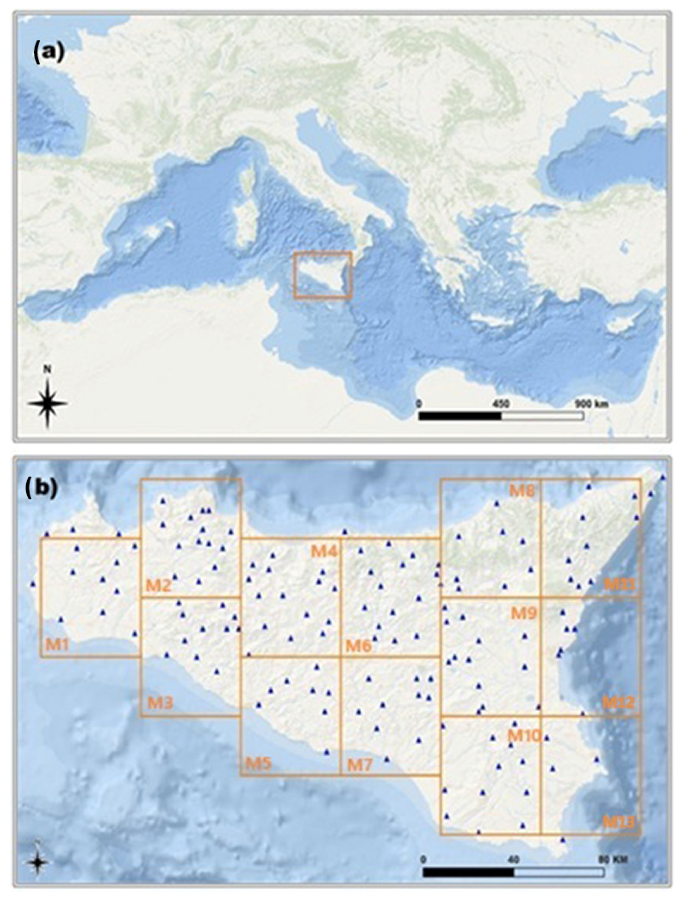
2.1. Area of Study

Sicily is the largest island in the Mediterranean Sea, with a total surface area of approximately 25,000 km². It extends in latitude between approximately 36° and 38° North and in longitude between approximately 12° and 15° East. The region is predominantly hilly, with 62% of its territory being hilly, 24% mountainous, and the remaining 14% flat. The orography of Sicily exhibits significant contrasts between its northern, mostly mountainous region, the central-southern and southwestern hilly region, the highland region in the southeast, and the volcanic region in the east. The hydrographic network on the island is complex, with dendritic-shaped river networks and basins of modest size. These characteristics are due to the compartmentalized structure of the island’s morphology, which favors the formation of a large number of independent river elements of limited development. The island has numerous torrential watercourses, many of which have a short and rapid course. The river valleys in the mountainous area are mostly narrow and deep, while they are considerably more open in the hilly zone. Sicily’s climate, classified as temperate–humid according to Köppen’s macroclimatic classification, is of type C, with an average coldest month temperature below 18 °C but above −3 °C. However, this definition only has macroclimatic value. On a regional scale, the climate is strongly influenced by local factors such as land formation, proximity to the coast, and orography [27]. According to [28,29], an analysis of Köppen’s type C temperate climate reveals several sub-types, including temperate subtropical, temperate warm, temperate sublittoral, temperate sub-continental, and temperate cool. These sub-types are found in different areas of Sicily. The diverse geography of Sicily results in a complex range of climates throughout the year, affecting both temperature and precipitation [30]. The study area was partitioned using a grid with a spatial resolution of 0.50° × 0.50°, resulting in 13 meshes (Mn). This resolution was considered optimal given the distribution of meteorological stations within the area. A higher resolution (e.g., 0.25° × 0.25°) would have produced meshes in which only one meteorological station would be present, meaning punctual information. Conversely, a lower resolution (e.g., 0.75° × 0.75°) would result in the loss of information regarding localized precipitation events [31,32,33]. In several works, observed values available on a grid with the same resolution as the RCM simulations were utilized [34,35]. This approach facilitated the creation of a compatibility between the resolution of the observed data simulated data. Consequently, it was possible to highlight the small-scale pluviometric differences affecting the study area. The coordinates and mesh designation are presented in

Table 1. Coordinates and meshes identifier.

Mesh	Latitude [N]	Longitude [E]
M1	38.00°–37.50°	13.00°–12.50°
M2	38.25°–37.75°	13.50°–13.00°
M3	37.75°–37.25°	13.50°–13.00°
M4	38.00°–37.50°	14.00°–13.50°
M5	37.50°–37.00°	14.00°–13.50°
M6	38.00°–37.50°	14.50°–14.00°
M7	37.50°–37.00°	14.50°–14.00°
M8	38.25°–37.75°	15.00°–14.50°
M9	37.75°–37.25°	15.00°–14.50°
M10	37.25°–36.75°	15.00°–14.50°
M11	38.25°–37.75°	15.50°–15.00°
M12	37.75°–37.25°	15.50°–15.00°
M13	37.25°–36.75°	15.50°–15.00°

. Figure 1 provides a visual representation of the study area, including the grid and the spatial distribution of the weather stations.

2.2. Precipitation Dataset

The precipitation dataset analyzed in this study was derived from the network of the Sicilian Agrometeorological Information Service (SIAS) and the Regional Water Observatory. The automatic checking of data for obvious anomalies, such as values falling outside the expected range or time inconsistencies, was a key component of this system. This preliminary validation process enabled the identification of evident errors prior to conducting a comprehensive evaluation. The validation of data was performed manually by SIAS technical staff. This process involved a comparison of the data with historical data, and the use of statistical methods to identify and correct systematic or sporadic errors. The identification and correction of errors was performed in accordance established methods [36,37,38]. This process was facilitated by an advanced database that enabled statistical processing and the utilization of climate indices, such as the ETCCDI [39,40]. Subsequent to validation, these data have been employed to generate agro-meteorological bulletins, thematic maps and other information tools, available through the web portal http://www.sias.regione.sicilia.it (accessed on 9 March 2025).

For each meteorological station, the monthly precipitation series was constructed for the period from 1991 to 2020. This time interval corresponds to the 30-year reference period (benchmark) stipulated by the WMO [25,26]. Consequently, the data from the meteorological stations, situated within each mesh, were aggregated to make them comparable with the data simulated by the model. For each mesh, the precipitation series derived from the aggregation were compared with the precipitation series derived from the reanalysis and simulations. ERA5 reanalysis data was sought from Climate Data Store (CDS), including climate indicators for Europe from 1940 to 2100. The climate model implemented was MPI-ESM (Max Planck Institute Earth System Model), a particularly suitable model for analyzing climate change on a regional scale, including patterns of precipitation, drought, and changes in thermal regimes [41,42,43]. It simulates the behavior of the Earth’s entire climate system, including the interactions between the atmosphere, oceans, soils, and other components of the climate system. It has been designed to study global and regional climate change and to make predictions about how the climate might evolve in the future. Due to its high spatial resolution of 0.25° × 0.25°, it enables more detailed simulations, especially for extreme events and regional climate change. It is mainly used for analyzing climate change on a regional scale, including patterns of precipitation, droughts, and changes in temperature regimes. It allows predictions to be made about how the climate might evolve in response to different greenhouse gas (GHG) emission scenarios.

Future projections for RCP (Representative Concentration Pathways) scenarios were considered, with particular attention focused on the RCP 4.5 scenario, which considers moderate mitigation policies to reduce GHG emissions, and the RCP 8.5 scenario, which assumes no mitigation policies for GHG emissions. The reanalysis precipitation data for the RCP 4.5 and RCP 8.5 scenarios covered the 30-year period 1991–2020, while the future precipitation data covered the 30-year period 2021–2050 and 2051–2080. Using MatLab, version R2023b, scripts, data in netCDF format were extracted for areas with a spatial resolution of 0.50° × 0.50° in order to maintain spatial coherence with the mesh size [44].

2.3. Bias Adjusting

In order to ensure proper calibration and validation, it was necessary that the spatial resolution of both simulated and observed data was similar. In instances where both resolutions were found to be compatible, direct comparison was performed and appropriate statistical corrections were applied. In several works, gridded ground-based observed data with the same resolution as the RCM simulations have been used. In this study, statistical relationships were interpreted as adjustment methods rather than downscaling techniques. The term “downscaling” refers to methods that improve the spatial resolution of a model from coarse to fine resolution. In this particular instance, however, the resolution of the adopted model was not increased. In order to adjust distortions in the model’s output data, linear scaling (LS) was adopted. The correction was performed through a scaling factor derived from the deviation between the observed and simulated series over the calibration period, as indicated by Equation (1):

$$P_{Adj,c}^{\ast }\left(m\right)=P_{Sim,c}\left(m\right){\displaystyle \frac{\mu P_{Obs,c}\left(m\right)}{\mu P_{Sim,c}\left(m\right) }}$$

(1)

where $P_{Adj,c}^{\ast }\left(m\right)$ is the adjusted monthly precipitation over the calibration period; $P_{Sim, c}\left(m\right)$ is the simulated monthly precipitation over the calibration period; $\mu P_{Obs,c}\left(m\right)$ is the average monthly precipitation observed over the calibration period; $\mu P_{Sim,c}\left(m\right)$ is the average simulated monthly precipitation over the calibration period.

The method was not utilized to modify the structural design of the model; rather, it was used to adjust the results in order to improve the realism and representativeness of the actual observations [45,46,47,48]. The goodness of fit of the model to the observed series was determined by applying the non-parametric Kolmogorov–Smirnov (KS) test to two samples [49,50]. The KS test permitted the comparison of the difference (D) between the cumulative distribution functions (CDF) of two samples. The null hypothesis (H₀) assumed that the values of the two data sets originated from a shared continuous distribution, while the alternative hypothesis (H_A) postulated that the values originated from distinct distributions. An hypothesis test can be performed at a specific level of statistical significance (e.g., 5%). In instances where the maximum distance between the two CDFs is sufficiently small, there is an absence of evidence to reject the null hypothesis (H₀) and consequently, the two series are regarded as originating from the same distribution (Equation (2)). It is important to note that two series originating from the same distribution are subject to the same probabilistic laws and thus exhibit similar behavior.

$$D=max\left[F\left(x\right)-G\left(x\right)\right]$$

(2)

2.4. Calculation of Pluviometric Deficit

The Standard Precipitation Index (SPI) is one of the most commonly used statistical indices for measuring drought in a given area. This index gives an indication of the relationship between the amount of precipitation that falls in a given time interval (t) and its climatological norm; this makes it possible to define whether the monitored area is affected by drought conditions or not, since the greater the distance from the norm, the greater the severity of the event. The Standardized Precipitation Index (SPI) calculation requires a long time series of at least 30 continuous years of monthly precipitation, as recommended by the WMO [51]. The SPI is calculated by analyzing a long-term precipitation series for a given location, aggregated over a given time interval. The aggregated precipitation series is interpolated using a gamma distribution. The precipitation time series X consists of n observations aggregated at time step t. For each $x>0$, the gamma distribution g(x) is defined by Equation (3):

$$g\left(x\right)={\displaystyle \frac{1}{{\beta }^{\alpha }\mathsf{\Gamma }\left(\alpha \right)}}{x}^{\alpha -1} e^{-{\displaystyle \frac{x}{\beta }}} \mathrm{w}\mathrm{i}\mathrm{t}\mathrm{h} \alpha > 0 \mathrm{a}\mathrm{n}\mathrm{d} \beta > 0$$

(3)

where α is the shape parameter, β is the scale parameter, and Γ(α) is the gamma function. Interpolation is achieved through optimal estimation of the parameters α and β, obtained using the maximum likelihood method, as illustrated in Equation (4):

$$\widehat{\alpha }={\displaystyle \frac{1}{4A}}\left(1+\sqrt{1+{\displaystyle \frac{4A}{3}}}\right)$$

(4)

where

$$A=\ln \left(\overline{x}\right)-{\displaystyle \frac{1}{n}}{\sum }_n\ln \left(x\right) \widehat{\beta }={\displaystyle \frac{\overline{x}}{\widehat{\alpha }}}$$

and $\overline{x}$ is the average of the n precipitation observations. The longer the series used to calculate the parameters of the distribution, the greater the robustness of the estimates obtained for the parameters of the g(x) distribution. Panofsky and Wilson [52] defined the cumulative probability distribution as shown in Equation (5):

$$G\left(x\right)={\int }_0^{x}g\left(x\right)dx={\displaystyle \frac{1}{{\widehat{\beta }}^{\widehat{\alpha }}\mathsf{\Gamma }\left(\widehat{\alpha }\right)}}{\int }_0^x{x}^{\alpha -1}{e}^{-{\displaystyle \frac{x}{\widehat{\beta }}}} dx$$

(5)

As the gamma distribution is undefined for $x=0$ and the zeros in the cumulative precipitation series represent periods of no rainfall, the gamma distribution is redefined by Equation (6):

$$H\left(x\right)=q+\left(1-q\right)G\left(X\right)$$

(6)

with $q={\displaystyle \frac{m}{n}}$, where q represents the probability of no precipitation, which can be estimated as the ratio of the number of zeros (m) in the precipitation time series to the total number of precipitation observations (n). The transformation of the cumulative distribution H(x) into a normal distribution result in a mean value of 0 for the SPI of a given location and aggregation period [53]. Computationally, the SPI value can be approximated by converting the cumulative distribution H(x) of the time series X to that of a normal random variable Z, as shown in Equation (7):

$$Z=SPI=\left\{\begin{array}{c}-\left(h-{\displaystyle \frac{c_0+c_{1}h+c_2{h}^2}{1+d_{1}h+d_2{h}^2+d_3{h}^3}}\right) for 0<H\left(x\right)\le 0.5\\ +\left(h-{\displaystyle \frac{c_0+c_{1}h+c_2{h}^2}{1+d_{1}h+d_2{h}^2+d_3{h}^3}}\right) for 0.5<H\left(x\right)\le 1\end{array}\right.$$

(7)

with $h=\left\{\begin{array}{c}\sqrt{\ln \left({\displaystyle \frac{1}{{\left(H\left(x\right)\right)}^2}}\right)} for 0<H\left(x\right)\le 0.5\\ \sqrt{\ln \left({\displaystyle \frac{1}{{\left(1-H\left(x\right)\right)}^2}}\right)} for 0.5<H\left(x\right)\le 1\end{array}\right.$, and

$$\begin{array}{ccc}{c}_0=2.5155& c_1=0.8028& c_2=0.0103\\ d_1=1.4327& d_2=0.1892& d_3=0.0013\end{array}$$

The Standardized Precipitation Index (SPI) typically ranges between +2 and −2, although values beyond these extremes are possible [54]. Negative values indicate a precipitation deficit, (drought), while positive values indicate a precipitation surplus, as shown in

Table 2. SPI classification scheme.

SPI Value	Classification
2.0 < SPI ≤ max	Extremely wet
1.5 < SPI ≤ 2.0	Very wet
1.0 < SPI ≤ 1.5	Moderately wet
0.0 < SPI ≤ 1.0	Mildly wet
−1.0 < SPI ≤ 0.0	Mildly dry
−1.5 < SPI ≤ 1.0	Moderately dry
−2.0 < SPI ≤ 1.5	Very dry
min < SPI ≤ −2.0	Extremely dry

[55]. The SPI’s normalization allows comparison between areas with different climatologies.

3. Results and Discussion

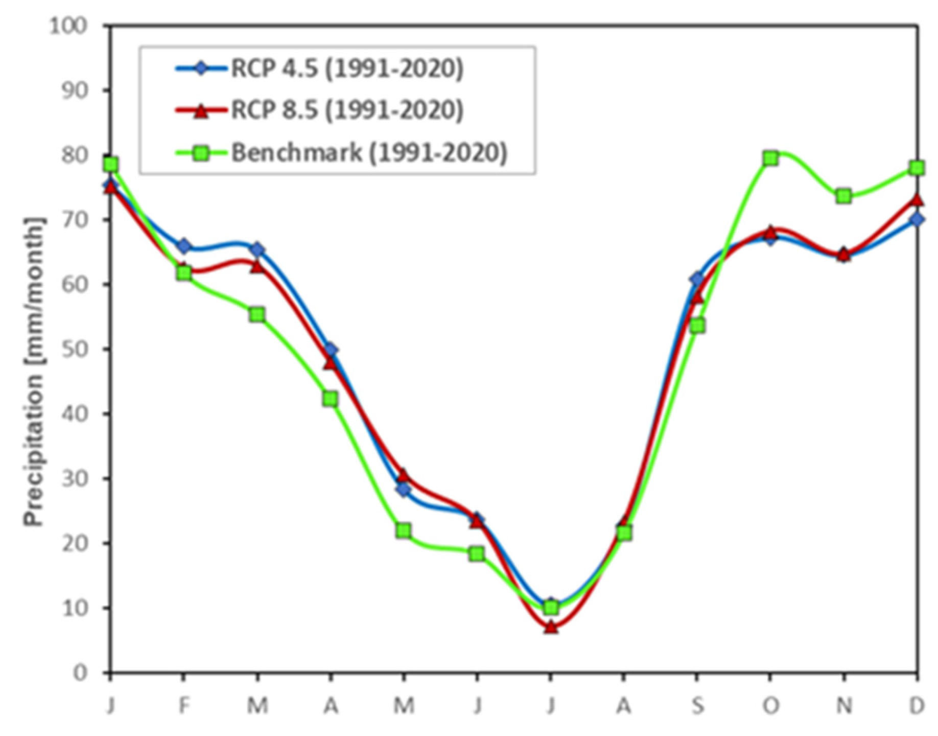
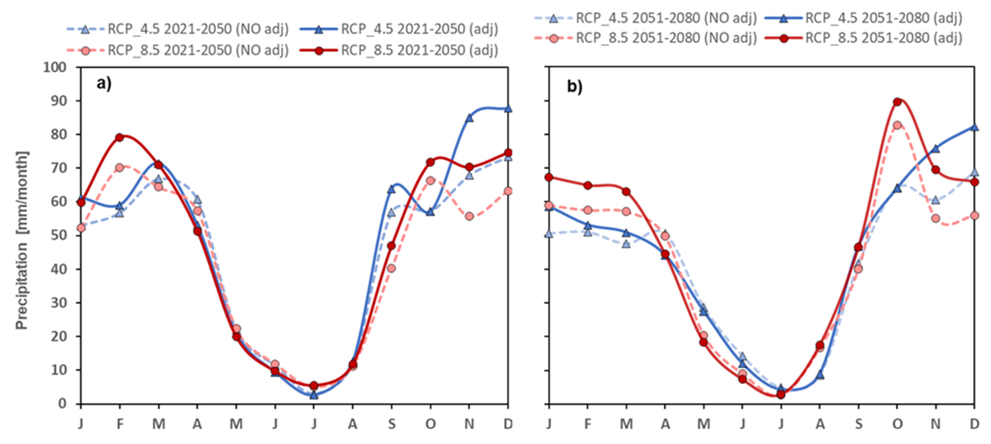
3.1. Climatic Normal Values and Adjustment

The climatological normal values of the observed monthly precipitation, as well as those for the RCP 4.5 and RCP 8.5 scenarios, were calculated with reference to the 1991–2020 (benchmark) period. As presented in Figure 2, a comparison was made between the normal climatic values obtained for mesh M9 and the respective climatic scenarios for the reference period. The mesh M9 was selected for analysis as it represents an area of agricultural importance, with significant areas of vineyards and citrus groves, which are vulnerable to intense precipitation events and drought. These characteristics render the mesh a suitable case study for the analysis of precipitation trends and agro-climatic risks. Moreover, it is the sole instance of a mesh surrounded on all four sides by other meshes.

The values obtained thus provided a climatological reference point for the adjustment of the RCP 4.5 and RCP 8.5 scenarios for the periods 2021–2050 and 2051–2080, respectively.

The linear scaling method was applied to the 13 meshes, resulting in adjustment of the precipitation series for both scenarios. This adjustment was found to be minimal during spring and summer, with the trends of the series before and after the adjustment remaining coherent. However, during the autumn and winter months, this coherence was found to be reduced, as the trends of the adjusted scenarios indicated an overestimation of monthly precipitation, as demonstrated also to [56,57]. The majority of the models demonstrate a tendency to overstate the frequency and intensity of precipitation during periods of the year when low temperatures and precipitation are observed. Figure 3 illustrates the RCP scenarios for mesh M9 before and after adjustment.

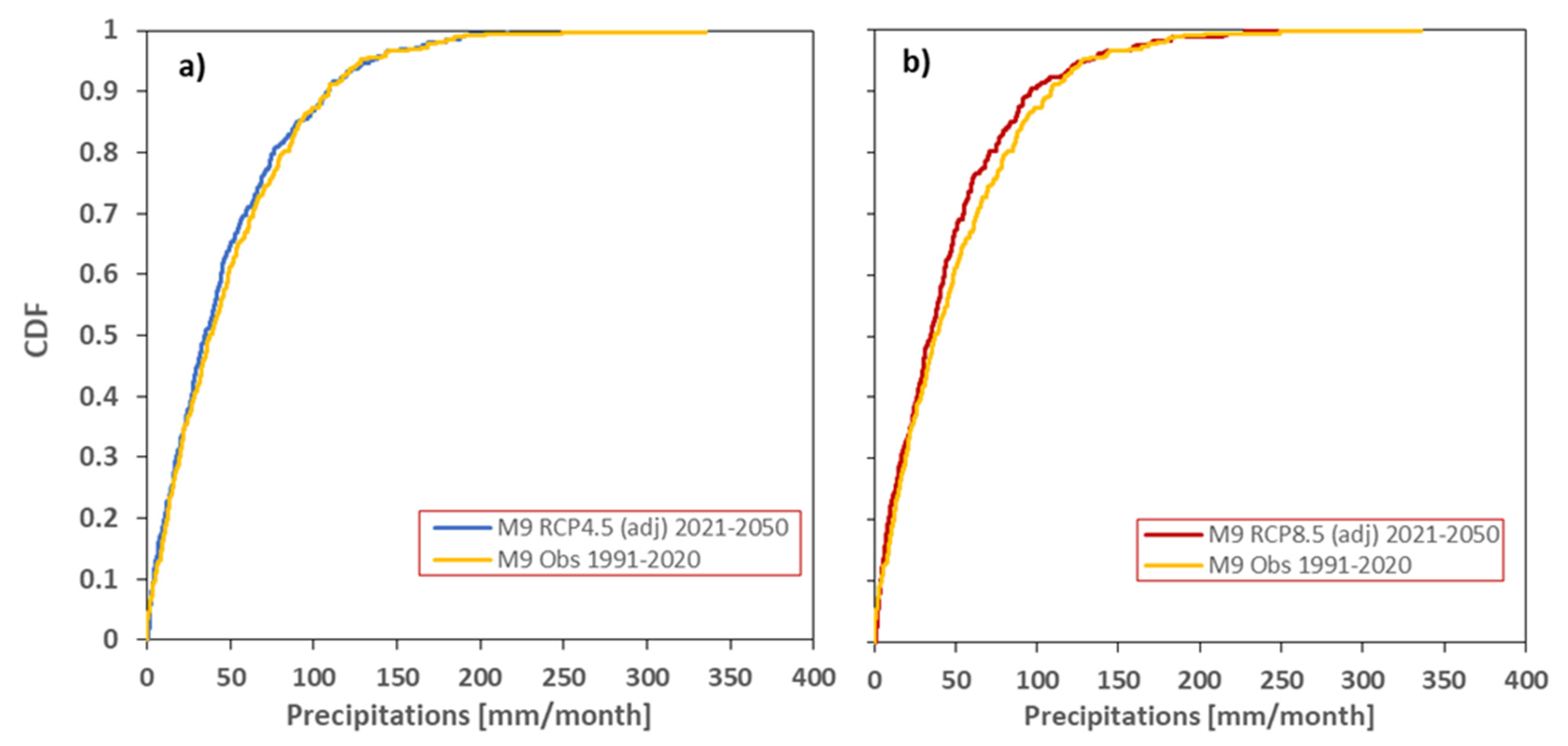
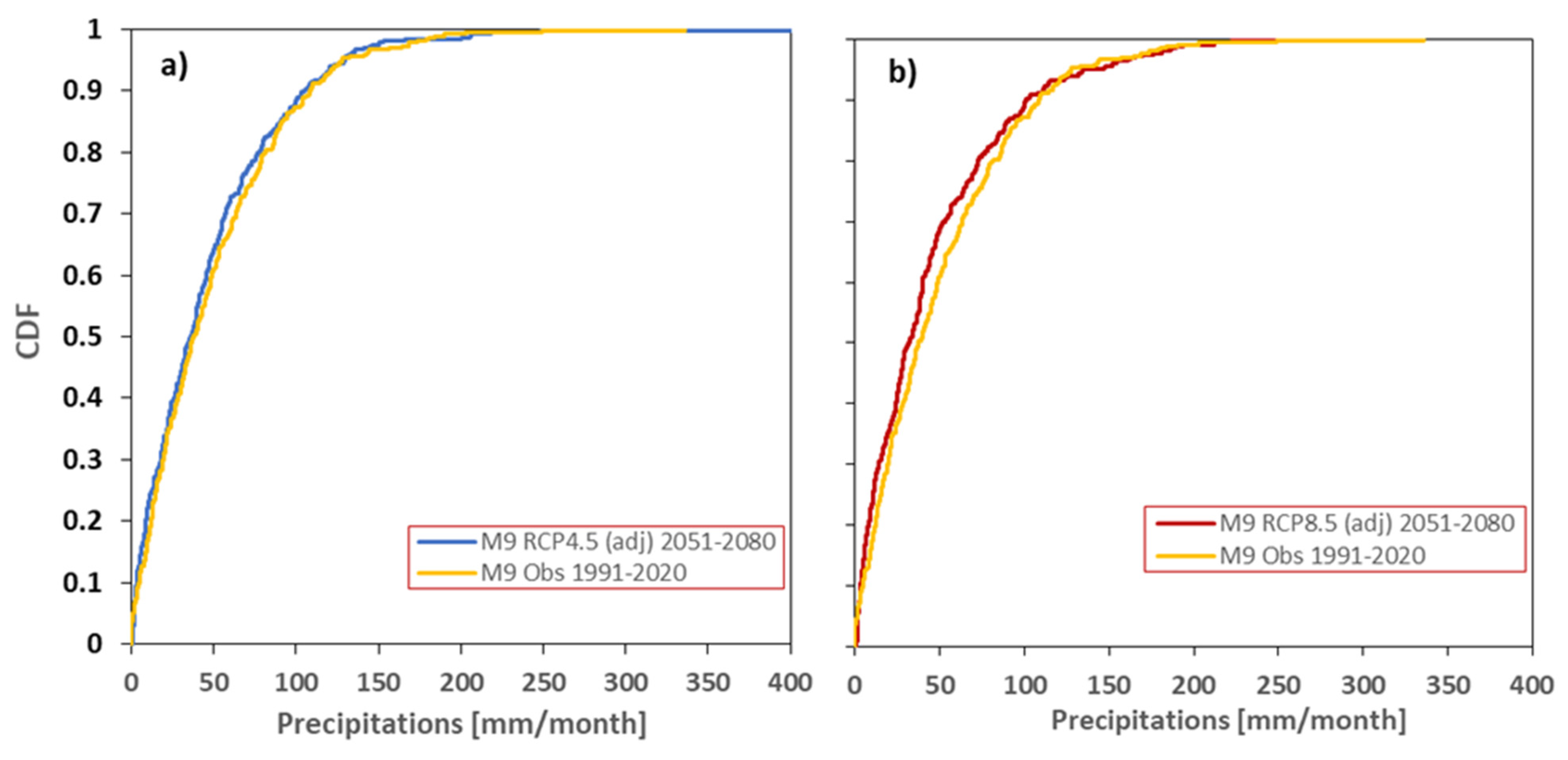
3.2. Kolmogorov–Smirnov Test Interpretation

In order to assess the goodness of fit of the observed precipitation series (Obs) to the adjusted RCP scenario series (adj), the Kolmogorov–Smirnov test was applied. In detail, the precipitation series (Obs) was compared with the RCP 4.5_(adj) 2021–2050, RCP 8.5_(adj) 2021–2050, RCP 4.5_(adj) 2051–2080 and RCP 8.5_(adj) 2051–2080 series for a significance level α = 0.05. The null hypothesis, denoted by H₀, asserts the similarity of the distribution of the two samples, while the alternative hypothesis, denoted by H_A, asserts their dissimilarity. Comparison of the (Obs) and (adj) series of RCPs for the 30-year period from 2021 to 2050 suggests that the distributions of the series are identical. This is evidenced by the p-value in all 13 meshes exceeding the significance level, as presented in

Table 3. Results of the Kolmogorov–Smirnov statistical method for a significance level α = 0.05 for the 30-year period 2021–2050. The results show that the null hypothesis H₀ is accepted for both scenarios in all meshes.

Obs—RCP 4.5(adj)				Obs—RCP 8.5(adj)
Id. Mesh	D	p-Value	Test Interpretation	Id. Mesh	D	p-Value	Test Interpretation
M1	0.075	0.264	Acept H0	M1	0.078	0.226	Acept H0
M2	0.053	0.698	Acept H0	M2	0.067	0.401	Acept H0
M3	0.058	0.573	Acept H0	M3	0.078	0.226	Acept H0
M4	0.078	0.226	Acept H0	M4	0.099	0.052	Acept H0
M5	0.078	0.226	Acept H0	M5	0.097	0.067	Acept H0
M6	0.056	0.635	Acept H0	M6	0.061	0.513	Acept H0
M7	0.067	0.401	Acept H0	M7	0.083	0.164	Acept H0
M8	0.067	0.401	Acept H0	M8	0.081	0.193	Acept H0
M9	0.056	0.635	Acept H0	M9	0.083	0.164	Acept H0
M10	0.064	0.455	Acept H0	M10	0.067	0.401	Acept H0
M11	0.039	0.949	Acept H0	M11	0.050	0.760	Acept H0
M12	0.047	0.817	Acept H0	M12	0.067	0.400	Acept H0
M13	0.069	0.350	Acept H0	M13	0.069	0.350	Acept H0

. However, for the 30-year period 2051–2080, there are some discrepancies between the RCP 4.5 scenario and the RCP 8.5 scenario. In the first scenario, the distributions under comparison are identical, and in all 13 meshes, the p-value exceeds the significance level. In the second scenario, in 6 meshes, the null hypothesis H₀ is rejected in favor of the alternative hypothesis H_A, meaning that the distributions are different as show in

Table 4. Results of the Kolmogorov–Smirnov statistical method for a significance level α = 0.05 for the 30-year period 2051–2080. These data show that the null hypothesis H₀ is accepted for the RCP 4.5 scenario in all meshes, while for the RCP 8.5 scenario it is rejected in 6 out of 13 meshes.

Obs—RCP 4.5(adj)				Obs—RCP 8.5(adj)
Id. Mesh	D	p-Value	Test Interpretation	Id. Mesh	D	p-Value	Test Interpretation
M1	0.097	0.067	Acept H0	M1	0.100	0.056	Acept H0
M2	0.094	0.081	Acept H0	M2	0.072	0.305	Acept H0
M3	0.089	0.116	Acept H0	M3	0.108	0.029	Reject H0
M4	0.101	0.056	Acept H0	M4	0.103	0.045	Reject H0
M5	0.094	0.081	Acept H0	M5	0.119	0.012	Reject H0
M6	0.086	0.139	Acept H0	M6	0.103	0.045	Reject H0
M7	0.092	0.097	Acept H0	M7	0.133	0.003	Reject H0
M8	0.069	0.350	Acept H0	M8	0.092	0.097	Acept H0
M9	0.058	0.573	Acept H0	M9	0.092	0.097	Acept H0
M10	0.086	0.139	Acept H0	M10	0.106	0.036	Reject H0
M11	0.044	0.870	Acept H0	M11	0.058	0.573	Acept H0
M12	0.053	0.698	Acept H0	M12	0.056	0.635	Acept H0
M13	0.067	0.400	Acept H0	M13	0.069	0.350	Acept H0

. Figure 4 and Figure 5 illustrate the cumulative distribution functions (CDF) for mesh M9 as an example.

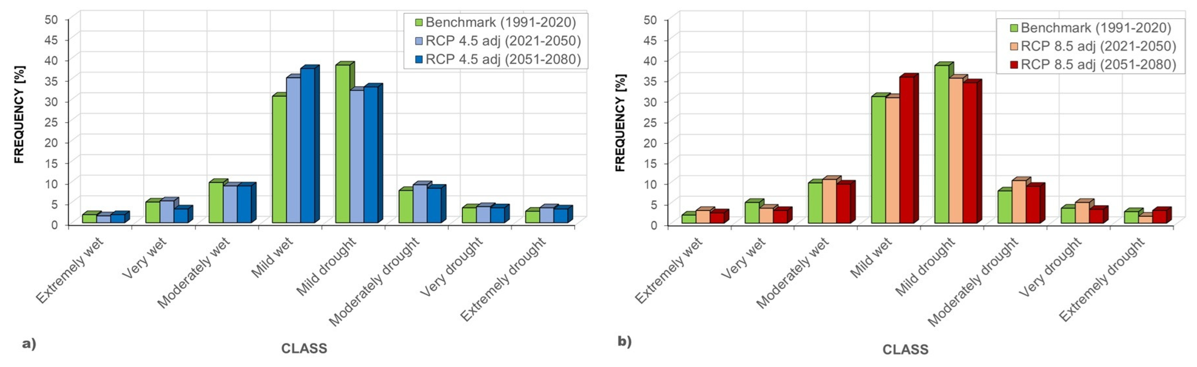
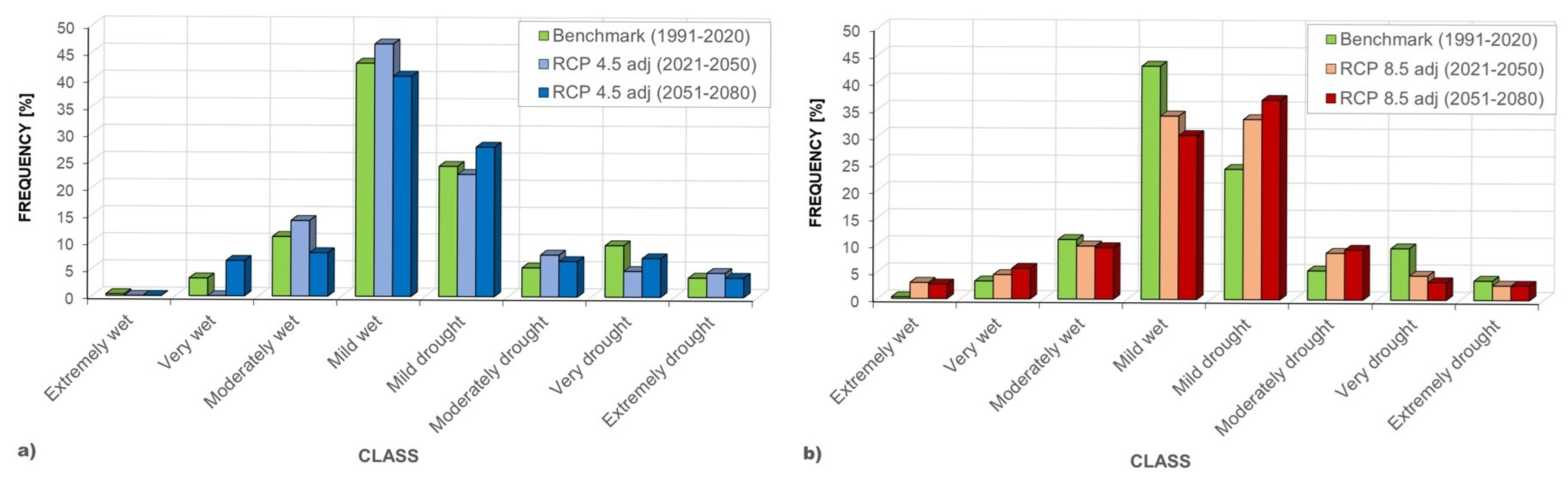
3.3. SPI Class Frequency Analysis

A frequency analysis for the Standardized Precipitation Index (SPI) categories was conducted. The SPI was utilised to evaluate drought, employing time intervals of 3, 12, and 24 months. According to Wilhite [24], these time periods are indicative of meteorological, hydrological, and socioeconomic drought.

The frequencies obtained for the RCP 4.5 and RCP 8.5 scenarios during the periods 2021–2050 and 2051–2080 were compared with the benchmark frequencies (1991–2020).

The analysis of the SPI_3-m index demonstrated marked short-term variability, particularly between the periods 2021–2050 and 2051–2080, and between the RCP 4.5 and RCP 8.5 scenarios. The frequent fluctuations between wet and dry conditions suggest an irregular distribution of precipitation, often concentrated in a limited number of days. This phenomenon is consistent with climate projections that indicate an increase in intense precipitation events and a decrease in moderate and distributed precipitation [58]. Such fluctuations can have significant impacts on seasonal water resources. Meshes such as M6, M7, M11, and M13 showed decreases in frequencies for the “extremely wet” and “very wet” classes, while others, such as M3, M4, and M9, showed increases in dry conditions for both scenarios. The increase in the “very dry” and “extremely dry” categories in many meshes indicates an increasing exposure to meteorological drought.

The results obtained for SPI_12-m indicated that, within the RCP 4.5 scenario, the alterations were less pronounced. Indeed, certain meshes, such as M5 and M10, showed an increase in wet conditions. However, in RCP 4.5 scenario, particularly during the period 2051–2080, a pronounced trend towards rising aridity and declining precipitation was evident. Meshes M6, M8, and M11 demonstrated a decline in the “extremely wet” classes, while meshes such as M3, M5, and M10 showed an increase, indicating varied behaviour across the distinct zones. It is noteworthy that the “moderately wet” category showed a decline in a significant portion of the area, indicating a potential reduction in the intermediate precipitation band, which may be indicative of an increase in extreme weather conditions. The increases in the classes “very dry” for M1, M10 and “extremely dry” for M2, M4, M5, indicate an increasing risk of persistent rainfall deficits, with effects on long-term water resources.

Finally, SPI_24-m for the RCP 4.5 scenario, period 2021–2050, showed a decrease in the “very wet” class at the expense of an increase in the “moderately wet” and “extremely dry” classes. In RCP 8.5 scenario, period 2051–2080, a clear shift towards drier conditions emerged, particularly evident in meshes such as M6, M8, M11, and M12. The decrease in the proportion of the “very wet” and “moderately wet” classes was accompanied by an increase in the “moderately dry”, “very dry”, and “extremely dry” categories in many cases, involving almost all meshes. This indicates a potential transition to persistent dry conditions, with direct implications for long-term water security. It is evident that meshes M4, M6 and M8 remain particularly vulnerable. The increased frequency of extreme drought conditions in almost all the meshes, with the exception of M10 and M13, suggests that, in the absence of adaptation actions, large areas could face chronic water shortages, exacerbating existing agricultural, urban and ecosystem problems.

Figure 6, Figure 7 and Figure 8 illustrate an example of the class frequency distribution for mesh M9.

A summary of the percentage changes in frequency for the SPI_3-m, SPI_12-m, and SPI_24-m categories found in the 13 meshes as a function of period and scenario is presented in the

Table 5. Percentage change in frequency for the SPI 3-month categories found in the 13 meshes as a function of period and scenario.

	Scenario	M1	M2	M3	M4	M5	M6	M7	M8	M9	M10	M11	M12	M13
Extremely Wet	ΔRCP 4.5(21–50)	+0.3	+0.7	−1.4	+0.6	−2.0	−1.1	−1.4	+0.8	−0.3	+0.0	−2.5	−0.3	−1.1
	ΔRCP 4.5(51–80)	+0.3	+0.6	−1.1	+0.8	+0.8	−0.6	−1.4	+0.6	0.0	+0.8	−2.5	−1.1	−1.4
	ΔRCP 8.5(21–50)	+0.8	+0.6	−0.6	0.0	−0.8	−1.1	−1.7	+1.1	+1.1	−0.3	−2.8	+0.3	−1.7
	ΔRCP 8.5(51–80)	+1.1	+0.5	+0.8	+1.3	+0.3	−0.3	0.0	+0.6	+0.6	+0.6	−2.0	−0.3	−0.5
Very Wet	ΔRCP 4.5(21–50)	−0.8	−2.0	+3.1	−3.6	+0.6	+0.8	−0.6	+1.4	+0.3	−1.7	+1.7	+1.7	−2.5
	ΔRCP 4.5(51–80)	−1.1	−2.8	+0.8	−2.8	−3.4	+1.4	+0.6	+1.1	−1.7	−3.1	+0.8	+0.3	−1.4
	ΔRCP 8.5(21–50)	+0.6	−1.7	+2.2	−2.8	+0.3	+1.7	+1.4	+1.7	−1.4	−1.4	+3.2	+1.4	−0.3
	ΔRCP 8.5(51–80)	−1.1	−2.2	0.0	−4.5	−2.0	+0.3	−0.3	+0.8	−2.0	−0.6	+1.4	+2.0	−4.1
Moderately Wet	ΔRCP 4.5(21–50)	+0.3	+0.3	−3.4	+3.6	+1.7	0.0	+1.7	−1.4	−0.8	−1.1	−0.6	−1.4	+2.8
	ΔRCP 4.5(51–80)	−0.8	−1.1	−1.7	−0.8	+2.5	−3.6	−1.4	−2.2	−0.8	−1.7	−0.8	−0.6	+0.3
	ΔRCP 8.5(21–50)	−1.4	0.0	−4.7	+1.4	−0.3	−2.2	−0.6	−3.4	+0.8	+0.3	−0.6	−2.0	+3.9
	ΔRCP 8.5(51–80)	−0.8	−0.6	−4.2	+1.1	+0.6	−1.4	−2.2	−1.7	−0.3	−4.2	+0.6	−1.7	+5.6
Mildly Wet	ΔRCP 4.5(21–50)	+1.1	−0.8	+4.5	+2.0	+0.6	0.0	+3.4	−1.4	+4.5	+5.3	+2.2	+3.6	+3.9
	ΔRCP 4.5(51–80)	+3.6	+3.9	+3.9	+6.7	+1.1	+3.4	+4.5	+3.9	+6.7	+4.5	+3.9	+6.1	+7.5
	ΔRCP 8.5(21–50)	−0.3	−1.1	+8.7	+3.9	+3.9	+3.4	+4.2	+1.1	−0.3	+1.1	−2.0	0.0	−1.7
	ΔRCP 8.5(51–80)	+1.4	+0.3	+6.1	+4.7	−0.8	+2.8	+3.1	+2.0	+4.7	+4.7	0.0	−1.7	−2.1
Mildly Dry	ΔRCP 4.5(21–50)	−2.0	+2.0	−1.4	−2.5	+2.0	+2.8	−3.4	+1.1	−6.1	−3.1	−1.7	−5.0	−5.9
	ΔRCP 4.5(51–80)	−3.4	−1.1	0.0	−3.4	+1.4	+2.2	−3.4	−0.6	−5.3	+0.3	−0.6	−2.8	−7.3
	ΔRCP 8.5(21–50)	−0.6	+0.8	−7.5	−5.3	−4.5	−1.7	−8.4	−0.6	−3.1	−0.3	+0.8	+0.3	−2.5
	ΔRCP 8.5(51–80)	−0.8	+1.4	−2.2	−4.5	+4.7	+0.3	−0.6	−0.8	−4.2	+1.1	+2.0	+2.0	+0.4
Moderately Dry	ΔRCP 4.5(21–50)	+1.4	−1.1	−2.8	−0.6	−2.8	−4.7	−0.8	−1.7	+1.4	0.0	−2.0	0.0	+1.7
	ΔRCP 4.5(51–80)	+2.2	0.0	−3.4	−1.7	−2.0	−5.3	+0.6	−3.4	+0.6	−1.4	−2.8	−3.4	+2.5
	ΔRCP 8.5(21–50)	+1.4	+1.4	+2.0	+2.5	+2.0	−1.7	+5.3	−1.4	+2.5	+0.3	−0.8	−0.3	+1.4
	ΔRCP 8.5(51–80)	+0.6	+0.3	−0.8	+2.2	−2.2	−3.1	0.0	−1.1	+1.1	−2.2	−3.9	−2.0	+1.4
Very Dry	ΔRCP 4.5(21–50)	+1.7	+0.8	+0.6	−1.4	−1.7	+0.6	+0.6	+0.3	+0.3	−0.3	+1.4	+2.0	+2.0
	ΔRCP 4.5(51–80)	+0.6	−0.3	+0.6	0.0	−1.7	+1.1	+0.3	−0.6	0.0	−0.6	+0.3	−0.3	−0.8
	ΔRCP 8.5(21–50)	+0.6	+1.1	−0.8	+0.3	−0.6	+1.1	+0.8	+1.4	+1.4	+0.3	+0.8	+0.8	+2.5
	ΔRCP 8.5(51–80)	−1.4	−0.6	+1.1	+0.3	+0.3	+0.8	−0.8	+1.1	+0.3	+0.3	+1.7	−0.3	−2.2
Extremely Dry	ΔRCP 4.5(21–50)	−2.0	−1.1	+0.8	+2.0	+1.7	+1.7	+0.6	+0.8	+0.8	+0.8	+1.4	−0.6	−0.8
	ΔRCP 4.5(51–80)	−1.4	0.0	+0.8	+1.1	+1.1	+1.4	+0.3	+1.1	+0.6	+1.1	+1.7	+1.7	+0.6
	ΔRCP 8.5(21–50)	−1.1	−1.4	+0.8	0.0	0.0	+0.6	−1.1	0.0	−1.1	0.0	+0.6	−0.6	−1.7
	ΔRCP 8.5(51–80)	−1.4	−0.6	+1.1	+0.3	+0.3	+0.8	−0.8	+1.1	+0.3	+0.3	+1.7	−0.3	−2.2

,

Table 6. Percentage change in frequency for the SPI 12-month categories found in the 13 meshes as a function of period and scenario.

		M1	M2	M3	M4	M5	M6	M7	M8	M9	M10	M11	M12	M13
Extremely Wet	ΔRCP 4.5(21–50)	0.0	+0.9	+0.8	−1.4	0.0	−3.4	−0.3	−0.6	−0.3	+0.3	−4.3	−3.2	−0.9
	ΔRCP 4.5(51–80)	−2.3	−1.1	0.0	+0.3	+2.0	−2.3	+1.4	−2.0	+1.4	+2.0	−5.7	−2.0	−1.4
	ΔRCP 8.5(21–50)	+0.3	+1.6	+2.9	+2.0	+3.2	−0.9	0.0	−0.6	+2.3	+2.9	−4.9	+1.1	0.0
	ΔRCP 8.5(51–80)	+3.2	−1.1	+2.6	−0.9	+5.2	−1.1	+4.0	−1.7	+2.3	+3.7	−3.2	0.0	0.0
Very Wet	ΔRCP 4.5(21–50)	−2.3	−2.6	−2.6	−0.6	+0.6	+1.7	−1.1	+1.4	−1.1	−1.4	+2.3	+3.7	+1.4
	ΔRCP 4.5(51–80)	−1.1	−2.6	+0.6	−2.6	+0.6	−1.1	−0.6	−0.6	−1.4	−2.9	+2.6	+2.3	+0.9
	ΔRCP 8.5(21–50)	−1.4	−2.6	−3.2	−2.3	−2.6	+0.3	+1.1	+2.6	−1.1	−2.9	+2.6	+1.1	+2.0
	ΔRCP 8.5(51–80)	−3.7	+2.3	0.0	+1.4	+2.3	+1.7	+1.7	+4.0	−2.9	−1.7	+2.9	0.0	−1.4
Moderately Wet	ΔRCP 4.5(21–50)	−0.9	−0.9	+0.9	−0.9	−0.3	−2.6	−0.3	−5.2	+0.9	+1.1	+1.4	+2.6	−2.6
	ΔRCP 4.5(51–80)	0.0	+2.3	−4.0	−0.6	−6.0	+0.3	−3.4	+1.1	−1.7	+0.3	−0.9	+0.3	−1.1
	ΔRCP 8.5(21–50)	+0.6	−3.4	−4.6	−4.0	−3.4	−4.0	−5.2	−5.4	+0.6	−2.0	+6.9	−0.6	−4.9
	ΔRCP 8.5(51–80)	−1.4	−2.6	−6.3	−3.4	−10.3	−2.0	−8.9	−2.3	−0.6	−3.7	+0.9	+2.6	+2.9
Mildly Wet	ΔRCP 4.5(21–50)	+6.6	+5.4	+2.0	+9.2	0.0	+13.2	+4.6	+12.6	−0.3	+1.7	+12.9	+4.0	+8.9
	ΔRCP 4.5(51–80)	+6.9	+7.7	+3.7	+8.0	+4.0	+10.9	+4.9	+5.7	+3.4	+1.7	+18.3	+9.2	+12.3
	ΔRCP 8.5(21–50)	+2.9	+9.2	+5.7	+6.6	+1.4	+9.2	+4.9	+5.7	−8.9	+5.2	+3.4	−0.3	+10.6
	ΔRCP 8.5(51–80)	0.0	+3.7	+1.4	+4.6	−4.6	+5.4	−4.0	+0.9	−1.7	−0.6	+11.2	−4.0	+1.7
Mildly Dry	ΔRCP 4.5(21–50)	−5.7	−4.3	+2.6	−3.2	+0.9	−7.2	+0.3	−5.4	−2.6	−1.7	−14.6	−6.6	−11.7
	ΔRCP 4.5(51–80)	−2.9	−4.0	+2.6	+1.4	−0.3	−6.6	−0.9	+0.6	−5.2	−1.4	−16.6	−12.9	−14.6
	ΔRCP 8.5(21–50)	−2.0	−6.6	+4.3	+2.0	+3.7	−2.9	+3.2	−0.3	+6.9	−3.2	−13.8	−2.3	−12.9
	ΔRCP 8.5(51–80)	+1.4	−3.4	+1.7	+0.6	+7.7	−3.7	+6.3	−1.7	−0.6	−0.9	−18.6	0.0	−6.3
Moderately Dry	ΔRCP 4.5(21–50)	−1.4	+1.1	−4.3	−6.3	−0.9	−3.4	−3.4	−2.6	+4.9	−2.0	0.0	−2.0	+2.3
	ΔRCP 4.5(51–80)	−4.6	−2.9	−2.0	−9.2	+0.6	−4.3	−1.7	−4.9	+3.7	−0.6	−2.9	+0.3	+1.1
	ΔRCP 8.5(21–50)	−4.3	+0.3	−5.2	−4.3	−1.4	−2.0	−3.2	−1.4	+1.7	−0.3	+2.6	0.0	+2.6
	ΔRCP 8.5(51–80)	−1.4	+0.6	+4.0	−5.7	+4.0	−1.1	+5.4	−0.3	+8.6	+6.6	+5.7	+3.4	+4.6
Very Dry	ΔRCP 4.5(21–50)	+2.9	−1.1	−1.7	+0.6	−2.3	−1.1	−2.3	−2.0	−0.9	+0.9	−0.3	−0.9	+2.0
	ΔRCP 4.5(51–80)	+0.9	−3.4	−3.4	−0.6	−0.3	−0.3	+0.3	−2.9	+0.9	−0.6	+1.4	+0.9	+2.3
	ΔRCP 8.5(21–50)	+4.6	−1.4	−3.2	−2.0	−0.6	−2.0	−1.1	−2.0	+0.9	−1.1	+3.4	+1.4	+4.0
	ΔRCP 8.5(51–80)	+3.7	−1.1	−2.9	+2.0	−0.6	−0.3	−0.6	+2.0	0.0	−0.3	+1.4	−0.9	+0.9
Extremely Dry	ΔRCP 4.5(21–50)	−1.1	+1.4	+2.3	+2.6	+2.0	+2.9	+2.6	+1.7	−0.6	+1.1	+2.6	+2.3	+0.6
	ΔRCP 4.5(51–80)	+3.2	+4.0	+2.6	+3.2	−0.6	+3.4	0.0	+2.9	−1.1	+1.4	+3.7	+2.0	+0.6
	ΔRCP 8.5(21–50)	−0.6	+2.0	+3.2	+2.0	−0.3	+2.3	+0.3	+1.4	−2.3	+1.4	−0.3	−0.6	−1.4
	ΔRCP 8.5(51–80)	−1.7	+1.7	−0.6	+1.4	−3.7	+1.1	−4.0	−0.9	−5.2	−3.2	−0.3	−1.1	−2.3

and

Table 7. Percentage change in frequency for the SPI 24-month categories found in the 13 meshes as a function of period and scenario.

		M1	M2	M3	M4	M5	M6	M7	M8	M9	M10	M11	M12	M13
Extremely Wet	ΔRCP 4.5(21–50)	+0.9	−0.3	0.0	0.0	0.0	−3.0	0.0	−2.7	−0.3	0.0	−3.0	−0.6	−3.9
	ΔRCP 4.5(51–80)	+0.9	+1.5	+1.2	+2.7	0.0	−2.7	0.0	−2.1	−0.3	0.0	−1.5	−0.3	−3.9
	ΔRCP 8.5(21–50)	+0.3	0.0	+2.1	+2.4	+1.2	−1.8	0.3	−2.7	+2.7	+0.9	−2.7	0.0	−4.2
	ΔRCP 8.5(51–80)	+0.6	−0.3	+0.9	+0.9	+0.9	−3.0	+1.8	−2.4	+2.4	+3.3	−0.3	−0.9	−1.2
Very Wet	ΔRCP 4.5(21–50)	−2.7	−2.4	−0.6	−6.8	−5.3	−4.2	−5.3	+0.9	−3.3	−0.9	−0.9	−5.0	+2.1
	ΔRCP 4.5(51–80)	−4.5	−1.8	−1.5	−3.3	−0.3	0.0	−2.4	+3.9	+3.3	+1.5	+1.2	+1.2	+2.7
	ΔRCP 8.5(21–50)	−3.6	+1.8	−0.9	−0.9	−0.3	+3.0	−0.6	+5.6	+1.2	+1.2	+3.0	+4.5	+3.9
	ΔRCP 8.5(51–80)	−0.9	−0.6	−3.6	−3.0	+5.6	+4.2	+3.9	+6.8	+2.4	+2.7	+3.6	+3.3	+2.1
Moderately Wet	ΔRCP 4.5(21–50)	−2.7	0.0	−1.5	+5.6	+0.9	+3.0	+1.2	+7.4	+3.0	−2.1	−0.6	+3.0	+13.4
	ΔRCP 4.5(51–80)	−3.9	−4.2	−2.4	−1.2	−1.2	+3.0	+3.3	+3.0	−3.0	−3.9	−5.9	−2.1	+1.8
	ΔRCP 8.5(21–50)	−1.2	−8.0	−2.7	−3.9	−2.4	−6.5	+6.2	+1.2	−1.2	−3.3	−3.3	−5.0	+8.0
	ΔRCP 8.5(51–80)	−3.9	+0.6	−4.2	+3.6	−6.2	+2.4	+1.5	+2.7	−1.5	−4.2	−6.5	−3.6	+8.6
Mildly Wet	ΔRCP 4.5(21–50)	+18.4	+14.5	+7.1	+6.5	+11.6	+15.4	+7.4	−5.6	+3.6	+7.4	+2.4	+8.6	−11.3
	ΔRCP 4.5(51–80)	+13.9	+11.9	+4.5	−0.3	+6.2	+4.2	−2.7	−9.2	−2.4	+2.7	+9.8	+3.9	+5.9
	ΔRCP 8.5(21–50)	+11.9	+15.7	+6.2	0.0	−2.1	+13.9	−16.3	0.0	−9.2	−0.6	+2.1	−2.7	−5.6
	ΔRCP 8.5(51–80)	+3.6	+5.0	+1.5	−7.7	−10.7	−0.9	−14.2	−14.5	−12.8	−9.5	−1.8	−5.6	−16.0
Mildly Dry	ΔRCP 4.5(21–50)	−11.3	−13.9	−5.3	+2.1	−3.6	−5.3	+1.5	+3.0	−1.5	−2.7	+3.0	−4.5	−3.9
	ΔRCP 4.5(51–80)	−2.7	−4.5	−2.4	+11.6	−4.7	0.0	+3.0	+6.2	+3.6	−4.2	−6.2	+0.6	−14.8
	ΔRCP 8.5(21–50)	−7.1	−8.9	−8.0	+8.9	+3.0	−3.6	+12.5	+2.4	+9.2	+2.4	−0.3	+8.6	−6.5
	ΔRCP 8.5(51–80)	−2.7	−8.3	−2.1	+14.5	+14.5	+4.7	+15.1	+10.7	+12.8	+6.5	+2.7	+4.2	+0.6
Moderately Dry	ΔRCP 4.5(21–50)	−2.4	−1.2	0.0	−9.5	−2.4	−11.3	−0.9	−0.3	+2.4	−2.1	+2.7	−2.1	+5.3
	ΔRCP 4.5(51–80)	−5.0	−6.5	+3.3	−12.2	+1.8	−10.1	+3.0	−0.6	+1.2	+5.3	+0.3	−5.6	+5.0
	ΔRCP 8.5(21–50)	−4.2	−5.9	+5.6	−7.7	+1.8	−9.2	+3.3	−0.9	+3.3	−0.9	+0.6	−3.6	+1.8
	ΔRCP 8.5(51–80)	+2.7	−2.7	+4.7	−11.3	−3.9	−10.4	−1.5	−0.6	+3.9	+3.3	+3.3	+5.3	+7.1
Very Dry	ΔRCP 4.5(21–50)	−4.2	0.0	−2.4	−2.4	−4.7	+0.9	−8.9	−5.3	−4.7	+0.6	−2.4	−1.2	−1.5
	ΔRCP 4.5(51–80)	−3.6	+0.3	−3.9	−3.6	−3.3	+0.9	−6.5	−1.2	−2.4	−1.2	−0.6	+1.2	+4.2
	ΔRCP 8.5(21–50)	+0.6	+3.0	−3.0	−2.7	−1.5	0.0	−8.6	−5.3	−5.0	+0.9	−3.0	−2.4	+3.0
	ΔRCP 8.5(51–80)	−1.2	+6.5	+0.3	−2.1	+2.1	−1.5	−3.6	−5.3	−6.2	+1.8	−0.6	−1.8	+2.7
Extremely Dry	ΔRCP 4.5(21–50)	+5.6	+3.3	+2.7	+4.5	+3.6	+3.5	+5.0	+2.1	+0.9	−0.3	+3.0	+1.8	−0.3
	ΔRCP 4.5(51–80)	+4.7	+3.3	+1.2	+6.2	+1.5	+4.7	+2.4	0.0	0.0	−0.3	+3.0	+1.2	−0.9
	ΔRCP 8.5(21–50)	+3.3	+2.4	+0.6	+3.9	+0.3	+4.2	+3.3	+2.1	−0.9	−0.6	+3.6	+0.6	−0.3
	ΔRCP 8.5(51–80)	0.0	−0.3	−1.8	+5.0	−2.4	+4.5	0.0	+2.7	−0.9	−3.9	−0.3	−2.7	−3.9

; positive changes (Δ > 0) indicate an increase in frequency of a class, conversely negative values (Δ < 0) indicate a decrease.

The analysis of the SPI on different time scales revealed marked spatial and temporal variability of drought conditions, especially between the different climate scenarios considered (RCP 4.5 and RCP 8.5). A thorough analysis of precipitation trends revealed a heightened degree of similarity in the seasonal variation of rainfall between the various meshes during the spring and summer months. This finding suggests a tendency towards a decrease in precipitation. This uniform behavior suggests greater consistency in climatic responses during the warmer months, potentially linked to greater atmospheric stability on a regional scale. Conversely, the cold seasons demonstrated increased spatial heterogeneity, with the meshes exhibiting divergent behavior. This phenomenon could be attributed to the influence of local meteorological phenomena, such as orographic precipitation, exerting a distinct effect on local climate trends [59]. Furthermore, this variability is reflected in the normal climate values, which renders the application of bias adjustment methodologies in the winter months more complex.

4. Conclusions

The study provides a thorough assessment of the evolution of drought conditions in the analyzed area through the use of the Standardized Precipitation Index (SPI) at different temporal scales, with reference to the RCP 4.5 and RCP 8.5 climate scenarios for the periods 2021–2050 and 2051–2080, respectively.

The results indicate a growing instability of the precipitation regime on a short-term basis (three-month SPI_3-m), characterized by frequent transitions between wet and dry conditions, frequently initiated by precipitation events concentrated over a limited number of days. This pattern is of particular significance for the domains of seasonal agriculture and the management of water resources over short timeframes. At the annual scale (SPI_12-m), there is a progressive decline in the frequency of moderately wet conditions and a corresponding increase in dry conditions, especially under the RCP 8.5 scenario. It is evident that certain grid cells are more vulnerable, indicating an escalating risk of protracted drought, with potential ramifications for agricultural, industrial, and civil water systems. At the biennial scale (SPI_24-m), the RCP 8.5 scenario evinces a discernible trend toward chronically arid conditions, indicating a structural criticality that is likely to intensify over time. Grid cells that already exhibit higher levels of drought susceptibility are projected to experience the most severe impacts in terms of frequency and duration of extreme drought events. The analysis of the SPI across different temporal scales has demonstrated that the tendency towards drought is increasing in both intensity and persistence as the time horizon extends, particularly under the RCP 8.5 scenario. The impacts are spatially heterogeneous, highlighting the need for localized and cross-sectoral adaptation strategies to effectively address future climate scenarios.

This study highlights the importance of monitoring precipitation variability over a range of temporal scales in order to detect early indications of drought. It also reveals the necessity of planning local adaptation measures based on the specific vulnerability of individual grid cells, taking into account their differentiated responses to climate scenarios. Consequently, the findings provide a valuable knowledge base to support the development of resilient territorial policies capable of responding to the challenges posed by climate change and increasing pressure on water resources.

The most efficient approach should include preventive measures to address precipitation deficits, such as the adoption of climate-resilient agricultural techniques and improved water management. Furthermore, it is imperative to cultivate adaptation capabilities at the territorial and regional levels. Interventions must be localized, taking into account the environmental, economic, and social particularities of each mesh. A multidisciplinary strategy integrating sustainable natural resource management policies with climate change adaptation strategies would offer a dual benefit, not only protecting the agricultural sector but also contributing to the overall resilience of the regional economy in the context of increasingly extreme climate scenarios.

References

1. Kushabaha, A.; Scardino, G.; Sabato, G.; Miglietta, M.M.; Flaounas, E.; Monforte, P.; Marsico, A.; De Santis, V.; Borzì, A.M.; Scicchitano, G. ARCHIMEDE—An innovative Web-GIS platform for the study of medicanes. Remote Sens. 2024, 16, 2552. [Google Scholar] [CrossRef]
2. Monforte, P.; Ragusa, M.A. Evaluation of bioclimatic discomfort trend in a central area of the mediterranean sea. Climate 2022, 10, 146. [Google Scholar] [CrossRef]
3. Wilhite, D.A. Planning for Drought: A Methodology. In Drought Assessment, Management, and Planning: Theory and Case Studies; Springer: Boston, MA, USA, 1993; pp. 87–108. [Google Scholar]
4. Vogt, J.V.; Niemeyer, S.; Somma, F.; Beaudin, I.; Viau, A.A. Drought monitoring from space. In Drought and Drought Mitigation in Europe; Springer: Berlin/Heidelberg, Germany, 2000; pp. 167–183. [Google Scholar]
5. Wilhite, D.A.; Glantz, M.H. Understanding: The drought phenomenon: The role of definitions. Water Int. 1985, 10, 111–120. [Google Scholar] [CrossRef]
6. Vogt, J.V.; Barbosa, P.; Cammalleri, C.; Carrão, H.; Lavaysse, C. Drought risk management: Needs and experiences in Europe. In Drought and Water Crises, Integrating Science, Management, and Policy; CRC Press: Boca Raton, FL, USA, 2017; pp. 385–407. [Google Scholar]
7. Colombo, T.; Pelino, V.; Vergari, S.; Cristofanelli, P.; Bonasoni, P. Study of temperature and precipitation variations in Italy based on surface instrumental observations. Glob. Planet. Change 2007, 57, 308–318. [Google Scholar] [CrossRef]
8. Brunetti, M.; Maugeri, M.; Nanni, T. Changes in total precipitation, rainy days and extreme events in northeastern Italy. Int. J. Climatol. A J. R. Meteorol. Soc. 2001, 21, 861–871. [Google Scholar] [CrossRef]
9. Homar, V.; Ramis, C.; Romero, R.; Alonso, S. Recent trends in temperature and precipitation over the Balearic Islands (Spain). Clim. Change 2009, 98, 199–211. [Google Scholar] [CrossRef]
10. de Luis, M.; Brunetti, M.; Gonzalez-Hidalgo, J.C.; Longares, L.A.; Martin-Vide, J. Changes in seasonal precipitation in the Iberian Peninsula during 1946–2005. Glob. Planet. Change 2010, 74, 27–33. [Google Scholar] [CrossRef]
11. Longobardi, A.; Villani, P. Trend analysis of annual and seasonal rainfall time series in the Mediterranean area. Int. J. Climatol. 2010, 30, 1538–1546. [Google Scholar] [CrossRef]
12. Matzneller, P.; Ventura, F.; Gaspari, N.; Pisa, P.R. Analysis of climatic trends in data from the agrometeorological station of Bologna-Cadriano, Italy (1952–2007). Clim. Change 2010, 100, 717–731. [Google Scholar] [CrossRef]
13. Brusca, S.; Famoso, F.; Lanzafame, R.; Messina, M.; Monforte, P. Placement optimization of biodiesel production plant by means of centroid mathematical method. Energy Procedia 2017, 126, 353–360. [Google Scholar] [CrossRef]
14. Brunetti, M.; Maugeri, M.; Monti, F.; Nanni, T. Temperature and precipitation variability in Italy in the last two centuries from homogenised instrumental time series. Int. J. Climatol. A J. R. Meteorol. Soc. 2006, 26, 345–381. [Google Scholar] [CrossRef]
15. Dai, A. Characteristics and trends in various forms of the Palmer Drought Severity Index during 1900–2008. J. Geophys. Res. Atmos. 2011, 116. [Google Scholar] [CrossRef]
16. Tsesmelis, D.E.; Leveidioti, I.; Karavitis, C.A.; Kalogeropoulos, K.; Vasilakou, C.G.; Tsatsaris, A.; Zervas, E. Spatiotemporal application of the standardized precipitation index (SPI) in the eastern Mediterranean. Climate 2023, 11, 95. [Google Scholar] [CrossRef]
17. Liu, C.; Yang, C.; Yang, Q.; Wang, J. Spatiotemporal drought analysis by the standardized precipitation index (SPI) and standardized precipitation evapotranspiration index (SPEI) in Sichuan Province, China. Sci. Rep. 2021, 11, 1280. [Google Scholar] [CrossRef]
18. Alley, W.M. The Palmer drought severity index: Limitations and assumptions. J. Appl. Meteorol. Climatol. 1984, 23, 1100–1109. [Google Scholar] [CrossRef]
19. Ampitiyawatta, A.D.; Wimalasiri, E.M. Review of Drought Characterization Indices. Sri Lankan J. Agric. Ecosyst. 2023, 5, 86–112. [Google Scholar] [CrossRef]
20. Stocker, T.F.; Qin, D.; Plattner, G.K.; Alexander, L.V.; Allen, S.K.; Bindoff, N.L.; Bréon, F.M.; Church, J.A.; Cubasch, U.; Emori, S.; et al. Technical summary. Climate change 2013: The physical science basis. In Contribution of Working Group I to the Fifth Assessment Report of the IPCC; Cambridge University Press: Cambridge, UK, 2013; pp. 33–115. [Google Scholar]
21. Monforte, P.; Ragusa, M.A. Temperature trend analysis and investigation on a case of variability climate. Mathematics 2022, 10, 2202. [Google Scholar] [CrossRef]
22. Caloiero, T.; Coscarelli, R.; Ferrari, E.; Sirangelo, B. Trend analysis of monthly mean values and extreme indices of daily temperature in a region of southern Italy. Int. J. Climatol. 2017, 37, 284–297. [Google Scholar] [CrossRef]
23. Fowler, H.J.; Blenkinsop, S.; Tebaldi, C. Linking climate change modelling to impacts studies. Int. J. Clim. 2007, 27, 1547–1578. [Google Scholar] [CrossRef]
24. Wilhite, D.A. Drought as a natural hazard: Concepts and definitions. In Droughts; Routledge: London, UK, 2016; pp. 3–18. [Google Scholar]
25. World Meteorological Organization. WMO Guidelines on the Calculation of Climate Normals (WMO-No.1203); World Meteorological Organization: Geneva, Switzerland, 2017; pp. 1–18. [Google Scholar]
26. World Meteorological Organization. Technical Regulations: WMO-No. 49; World Meteorological Organization: Geneva, Switzerland, 2019. [Google Scholar]
27. Littmann, T. An empirical classification of weather types in the Mediterranean Basin and their interrelation with rainfall. Theor. Appl. Climatol. 2000, 66, 161–171. [Google Scholar] [CrossRef]
28. Salata, F.; Golasi, I.; Treiani, N.; Plos, R.; Vollaro, A.d.L. On the outdoor thermal perception and comfort of a Mediterranean subject across other Koppen-Geiger’s climate zones. Environ. Res. 2018, 167, 115–128. [Google Scholar] [CrossRef] [PubMed]
29. Fratianni, S.; Acquaotta, F. The climate of Italy. In Landscapes and Landforms of Italy; Springer: Berlin/Heidelberg, Germany, 2017; pp. 29–38. [Google Scholar]
30. Bordi, I.; Fraedrich, K.; Petitta, M.; Sutera, A. Extreme value analysis of wet and dry periods in Sicily. Theor. Appl. Climatol. 2007, 87, 61–71. [Google Scholar] [CrossRef]
31. Weisse, A.K.; Bois, P. Topographic effects on statistical characteristics of heavy rainfall and mapping in the French Alps. J. Appl. Meteorol. 2001, 40, 720–740. [Google Scholar] [CrossRef]
32. Wilhere, G.F. Adaptive management in habitat conservation plans. Conserv. Biol. 2002, 16, 20–29. [Google Scholar] [CrossRef]
33. Tramblay, Y.; Neppel, L.; Carreau, J. Brief communication Climatic covariates for the frequency analysis of heavy rainfall in the Mediterranean region. Nat. Hazards Earth Syst. Sci. 2011, 11, 2463–2468. [Google Scholar] [CrossRef]
34. Piani, C.; Weedon, G.; Best, M.; Gomes, S.; Viterbo, P.; Hagemann, S.; Haerter, J. Statistical bias correction of global simulated daily precipitation and temperature for the application of hydrological models. J. Hydrol. 2010, 395, 199–215. [Google Scholar] [CrossRef]
35. Kurnik Blaž, L.; Bogataj, K.; Ceglar, A. Correcting mean and extremes in monthly precipitation from 8 regional climate models over Europe. Clim. Past Discuss. 2012, 8, 953–986. [Google Scholar]
36. Estévez, J.; Llabrés-Brustenga, A.; Casas-Castillo, M.C.; García-Marín, A.P.; Kirchner, R.; Rodríguez-Solà, R. A quality control procedure for long-term series of daily precipitation data in a semiarid environment. Theor. Appl. Climatol. 2022, 149, 1029–1041. [Google Scholar] [CrossRef]
37. Estévez, J.; Gavilán, P.; García-Marín, A.P. Data validation procedures in agricultural meteorology–a prerequisite for their use. Adv. Sci. Res. 2011, 6, 141–146. [Google Scholar] [CrossRef]
38. You, J.; Hubbard, K.G.; Nadarajah, S.; Kunkel, K.E. Performance of quality assurance procedures on daily precipitation. J. Atmos. Ocean. Technol. 2007, 24, 821–834. [Google Scholar] [CrossRef]
39. Dunn, R.J.; Donat, M.G.; Alexander, L.V. Comparing extremes indices in recent observational and reanalysis products. Front. Clim. 2022, 4, 989505. [Google Scholar] [CrossRef]
40. Tebaldi, C.; Armbruster, A.; Engler, H.P.; Link, R. Emulating climate extreme indices. Environ. Res. Lett. 2020, 15, 074006. [Google Scholar] [CrossRef]
41. Ibebuchi, C.C. The impact of horizontal resolution on the representation of atmospheric circulation types in Western Europe using the MPI-ESM model. Int. J. Climatol. 2023, 43, 6450–6462. [Google Scholar] [CrossRef]
42. Ibebuchi, C.C. Circulation type analysis of regional hydrology: The added value in using CMIP6 over CMIP5 simulations as exemplified from the MPI-ESM-LR model. J. Water Clim. Change 2022, 13, 1046–1055. [Google Scholar] [CrossRef]
43. Yulan, L.; Gong, H.; Chen, W.; Wang, L. Contribution of internal variability to the Mongolian Plateau summer precipitation trends in MPI-ESM large-ensemble model. Glob. Planet. Change 2024, 240, 104544. [Google Scholar]
44. Zhuk, E. Using GIS technology for visualizing marine environmental data in netCDF format. In Proceedings of the Ninth International Conference on Remote Sensing and Geoinformation of the Environment (RSCy2023), Ayia Napa, Cyprus, 3–5 April 2023; SPIE: Bellingham, WA, USA, 2023; Volume 12786. [Google Scholar]
45. Piani, C.; Haerter, J.C.; Coppola, E. Statistical bias correction for daily precipitation in regional climate models over Europe. Theor. Appl. Climatol. 2010, 99, 187–192. [Google Scholar] [CrossRef]
46. Themeßl, M.J.; Gobiet, A.; Leuprecht, A. Empirical-statistical downscaling and error correction of daily precipitation from regional climate models. Int. J. Climatol. 2011, 31, 1530–1544. [Google Scholar] [CrossRef]
47. Themeßl, M.J.; Gobiet, A.; Heinrich, G. Empirical-statistical downscaling and error correction of regional climate models and its impact on the climate change signal. Clim. Change 2012, 112, 449–468. [Google Scholar] [CrossRef]
48. Talchabhadel, R.; Aryal, A.; Kawaike, K.; Yamanoi, K.; Nakagawa, H.; Bhatta, B.; Karki, S.; Thapa, B.R. Evaluation of precipitation elasticity using precipitation data from ground and satellite-based estimates and watershed modeling in Western Nepal. J. Hydrol. Reg. Stud. 2021, 33, 10. [Google Scholar] [CrossRef]
49. Massey, F.J., Jr. The Kolmogorov-Smirnov test for goodness of fit. J. Am. Stat. Assoc. 1951, 46, 68–78. [Google Scholar] [CrossRef]
50. Lanzante, J.R. Testing for differences between two distributions in the presence of serial correlation using the Kolmogorov–Smirnov and Kuiper’s tests. Int. J. Clim. 2021, 41, 6314–6323. [Google Scholar] [CrossRef]
51. Svoboda, M.; Hayes, M.; Wood, D. Standardized Precipitation Index: User Guide; World Meteworological Organization: Geneva, Switzerland, 2012. [Google Scholar]
52. Panofsky, H.A.; Brier, G.W. Some Applications of Statistics to Meteorology; Pennsylvania State University: University Park, PA, USA, 1968. [Google Scholar]
53. Edwards, D.C.; McKee, T.B. Characteristics of 20th Century Drought in the United States at Multiple Time Scales; Colorado State University: Collins, CO, USA, 1997. [Google Scholar]
54. McKee, T.B.; Doesken, N.J.; Kleist, J. The relationship of drought frequency and duration to time scales. In Proceedings of the 8th Conference on Applied Climatology, Anaheim, CA, USA, 17–22 January 1993; Volume 17. [Google Scholar]
55. Nimisha, K.; Arunkumar, R. Meteorological drought analysis under climate change scenario using SPI index. In Proceedings of the International Conference on Emerging Trends in Engineering, Yukthi-2023, Kozhikode, India, 10–12 April 2023; Department of Civil Engineering, Government Engineering College: Kozhikode, India, 2023; pp. 394–400. [Google Scholar]
56. Addor, N.; Rohrer, M.; Furrer, R.; Seibert, J. Propagation of biases in climate models from the synoptic to the regional scale: Implications for bias adjustment. J. Geophys. Res. Atmos. 2016, 121, 2075–2089. [Google Scholar] [CrossRef]
57. Dosio, A.; Paruolo, P. Bias correction of the ENSEMBLES high-resolution climate change projections for use by impact models: Evaluation on the present climate. J. Geophys. Res. Atmos. 2011, 116. [Google Scholar] [CrossRef]
58. Pavan, V.; Antolini, G.; Barbiero, R.; Berni, N.; Brunier, F.; Cacciamani, C.; Torrigiani Malaspina, T. High resolution climate precipitation analysis for north-central Italy, 1961–2015. Clim. Dyn. 2019, 52, 3435–3453. [Google Scholar] [CrossRef]
59. Avanzi, F.; De Michele, C.; Gabriele, S.; Ghezzi, A.; Rosso, R. Orographic signature on extreme precipitation of short durations. J. Hydrometeorol. 2015, 16, 278–294. [Google Scholar] [CrossRef]
Figure 1. (a) The study area in the Mediterranean basin. (b) Location of the weather stations (blue triangles) and the 0.5° × 0.5° grid size that partitioned the area.
Hydrology 12 00143 g001
Figure 2. Comparison between the normal climatic values obtained for mesh M9 and the respective climatic scenarios for the reference period.
Hydrology 12 00143 g002
Figure 3. (a) Climatic normal values relative to monthly precipitation in M9 for the period 2021–2050. The RCP 4.5 scenario is represented by a dashed light blue line, while the RCP 4.5 scenario “adjusted” is shown by the solid blue line. The RCP 8.5 scenario is represented by a dashed pink line, and the RCP 8.5 scenario “adjusted” is represented by the solid red line. (b) Monthly precipitation normal climate values for the period 2051–2080, using the same fonts as in (a).
Hydrology 12 00143 g003
Figure 4. Cumulative distribution function (CDF) trend for mesh M9. (a) The distribution of the series (Obs) is represented with a yellow line, and with a blue line the distribution for the RCP 4.5 scenario for the 30-year period 2021–2050. (b) The distribution of the series (Obs) is represented with a yellow line, while the distribution for the RCP 8.5 scenario is represented with a red line for the 30-year period 2021–2050.
Hydrology 12 00143 g004
Figure 5. Cumulative distribution function (CDF) trend for mesh M9. (a) The distribution of the series (Obs) is represented with a yellow line, and with a blue line the distribution for the RCP 4.5 scenario for the 30-year period 2051–2080. (b) The distribution of the series (Obs) is represented with a yellow line, while the distribution for the RCP 8.5 scenario is represented with a red line for the 30-year period 2051–2080.
Hydrology 12 00143 g005
Figure 6. Frequency distribution of the SPI 3-month categories for mesh M9: (a) green bars indicate the benchmark (1991–2020), light blue bars correspond to the RCP 4.5 scenario (2021–2050), blue bars correspond to the RCP 4.5 scenario (2051–2080); (b) green bars indicate the benchmark (1991–2020), orange bars correspond to the RCP 8.5 scenario (2021–2050), dark red bars correspond to the RCP 8.5 scenario (2051–2080).
Hydrology 12 00143 g006
Figure 7. Frequency distribution of the SPI 12-months categories for mesh M9: (a) green bars indicate the benchmark (1991–2020), light blue bars correspond to the RCP 4.5 scenario (2021–2050), blue bars correspond to the RCP 4.5 scenario (2051–2080); (b) green bars indicate the benchmark (1991–2020), orange bars correspond to the RCP 8.5 scenario (2021–2050), dark red bars correspond to the RCP 8.5 scenario (2051–2080).
Hydrology 12 00143 g007
Figure 8. Frequency distribution of the SPI 24-months categories for mesh M9: (a) green bars indicate the benchmark (1991–2020), light blue bars correspond to the RCP 4.5 scenario (2021–2050), blue bars correspond to the RCP 4.5 scenario (2051–2080); (b) green bars indicate the benchmark (1991–2020), orange bars correspond to the RCP 8.5 scenario (2021–2050), dark red bars correspond to the RCP 8.5 scenario (2051–2080).
Hydrology 12 00143 g008