
Flood Risk Assessment Under Climate Change Scenarios in the Wadi Ibrahim Watershed


Abstract
1. Introduction
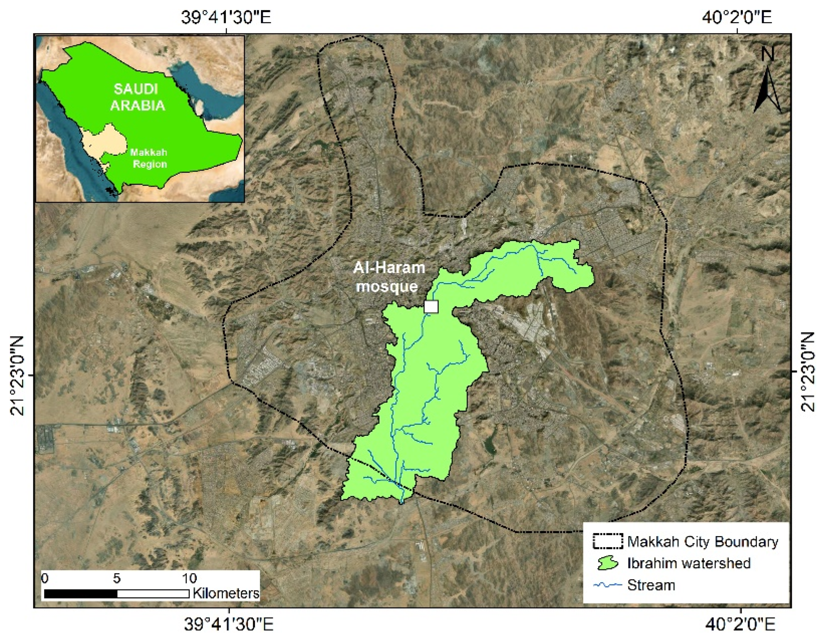
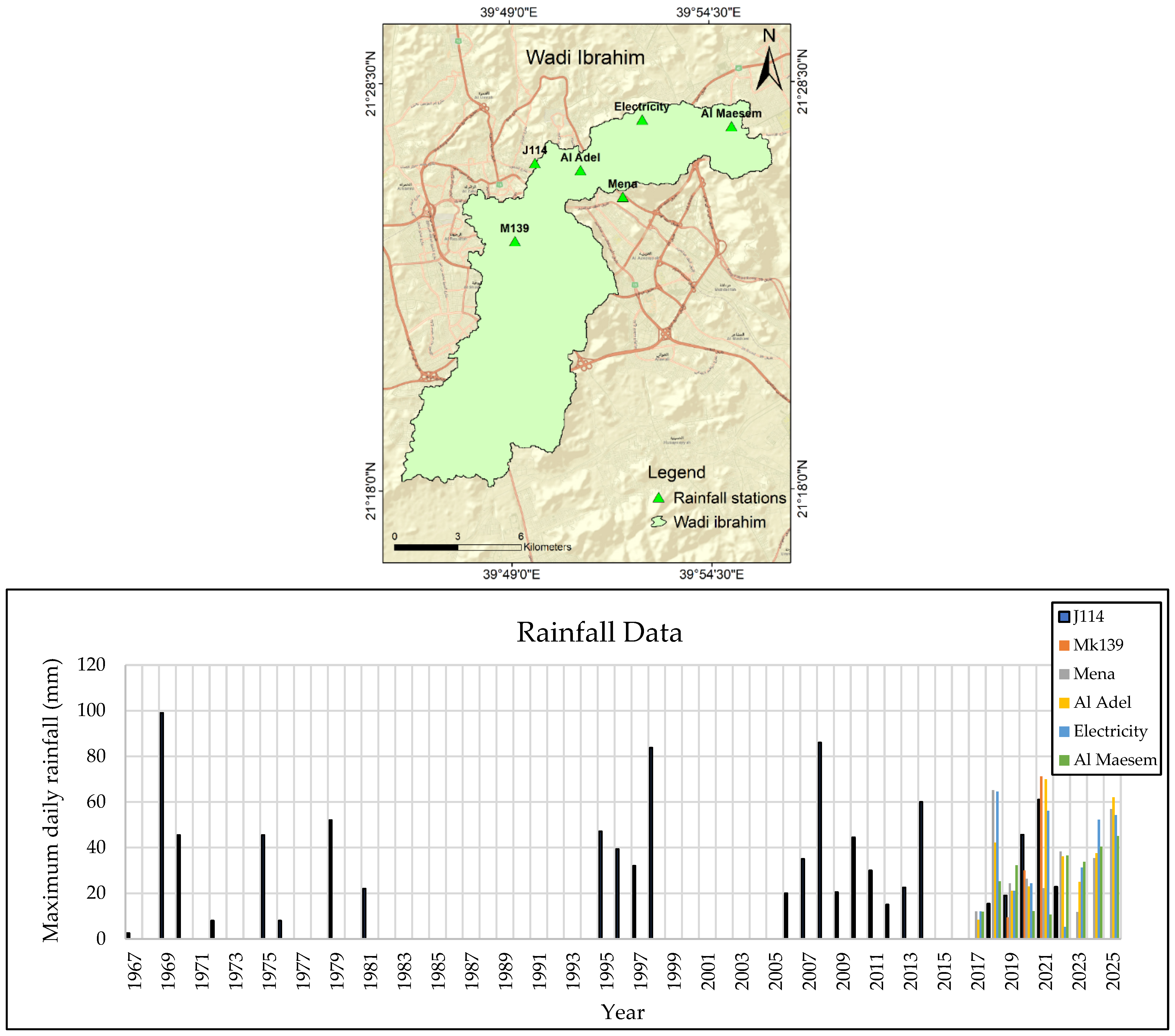
2. Study Area and Data Collection
3. Data Collection and Methodology
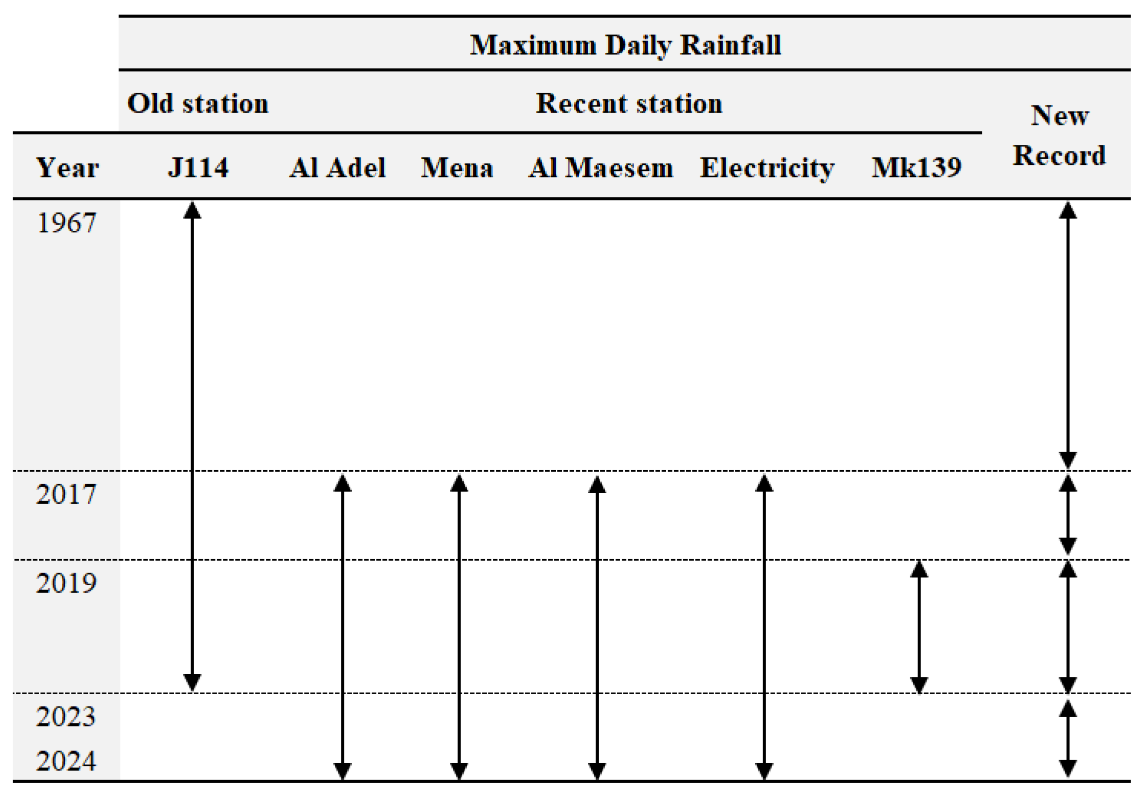
3.1. Data Collection
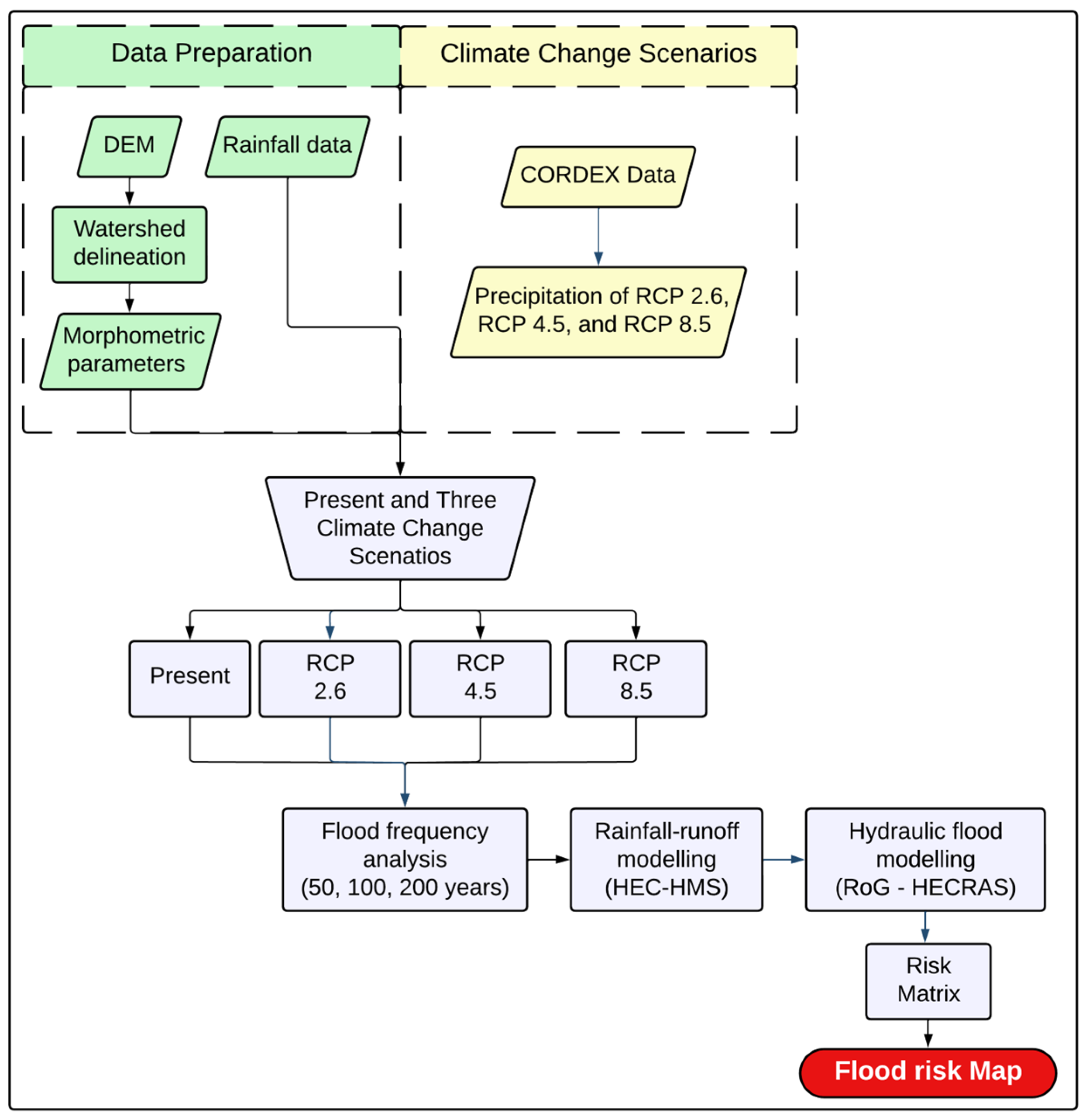
3.2. Methodology
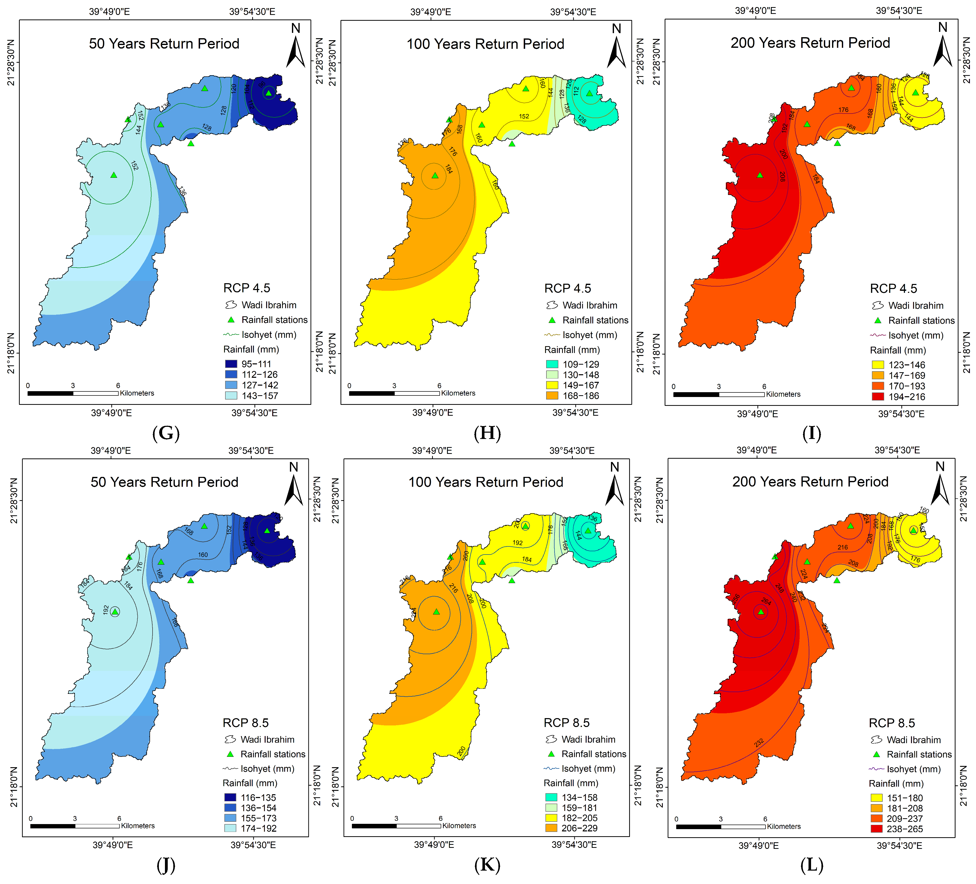
3.2.1. Rainfall Analysis
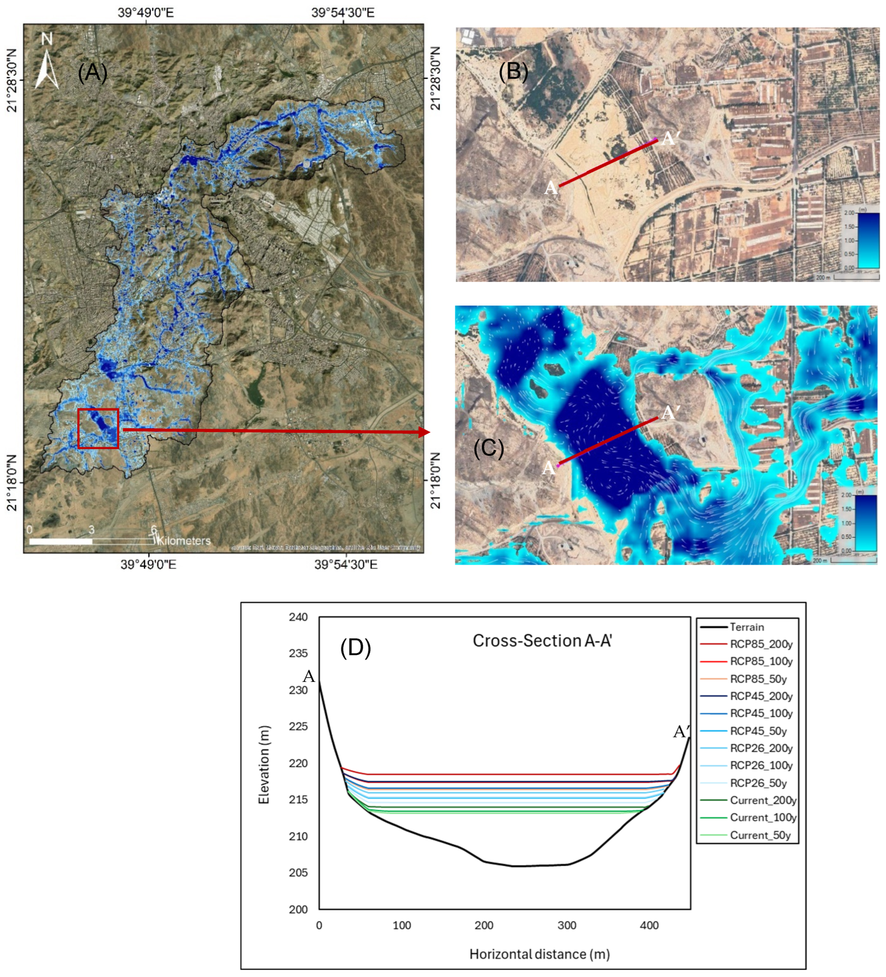
3.2.2. Hydraulic Modeling Using Rain-on-Grid (RoG)
3.2.3. Flood Risk Matrix
4. Results
5. Discussion
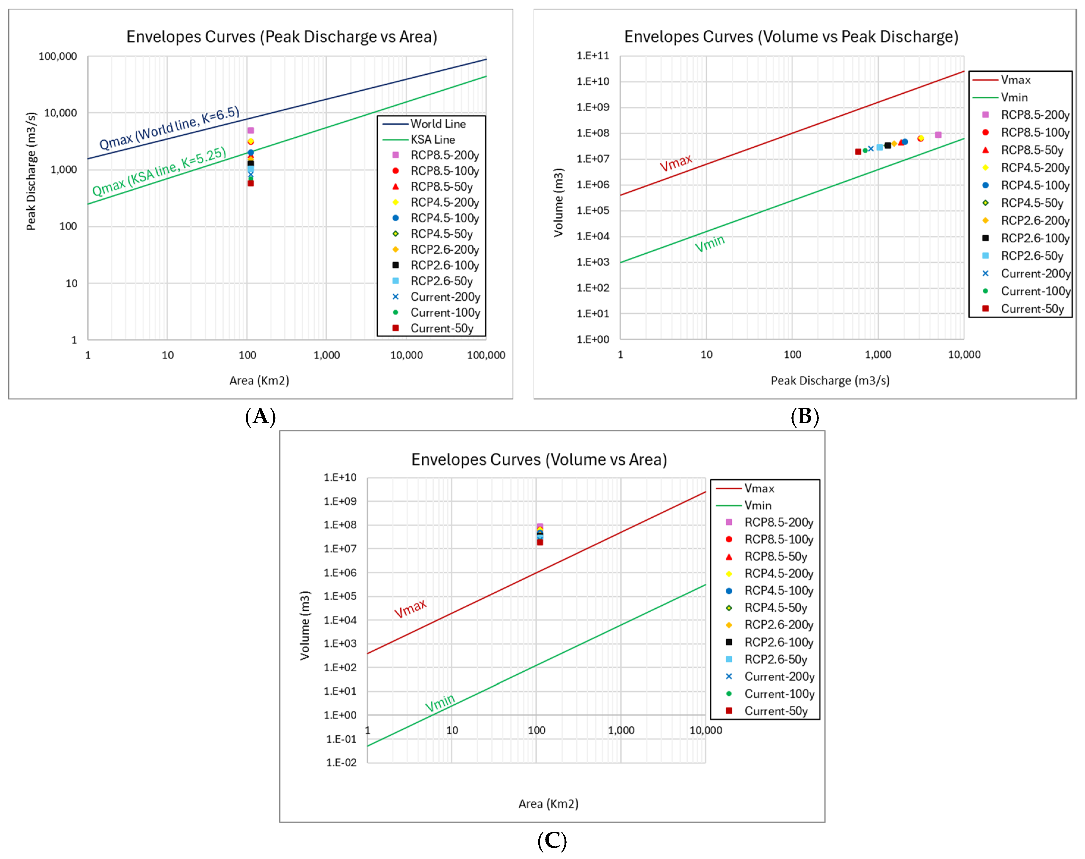
5.1. Envelope Curves for , A, and V
5.2. Practical Implications of the Flood Risk in an Arid Environment
6. Conclusions
- The rain-on-grid (RoG) model demonstrated reliable performance and logical consistency in simulating the flood dynamics across scenarios.
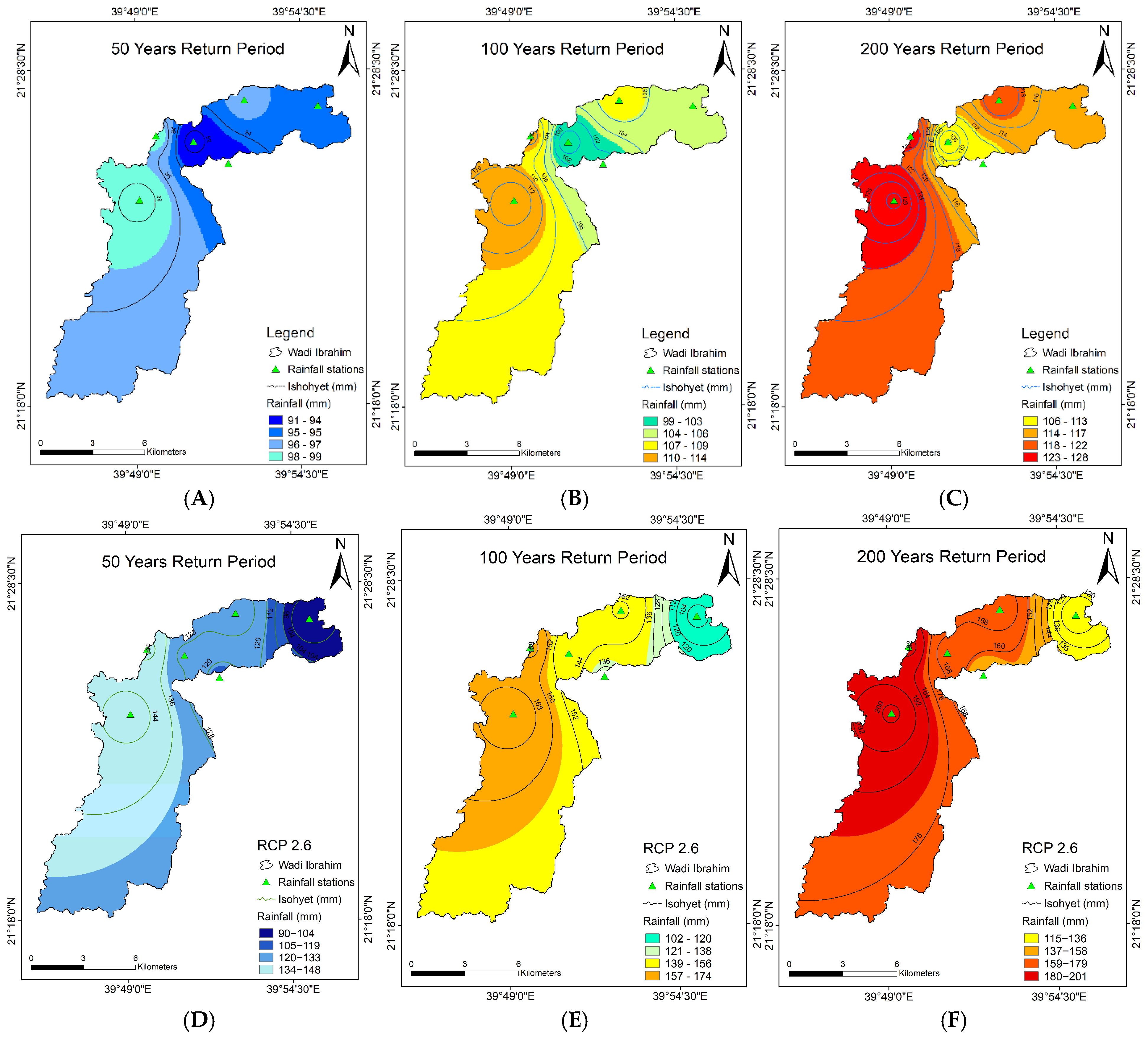
- Under current climate conditions, the flood volume increased significantly from 18,919 × 103 m3 (50-year return period) to 24,821 × 103 m3 (200-year return period), with an average flood depth of 0.2 m.
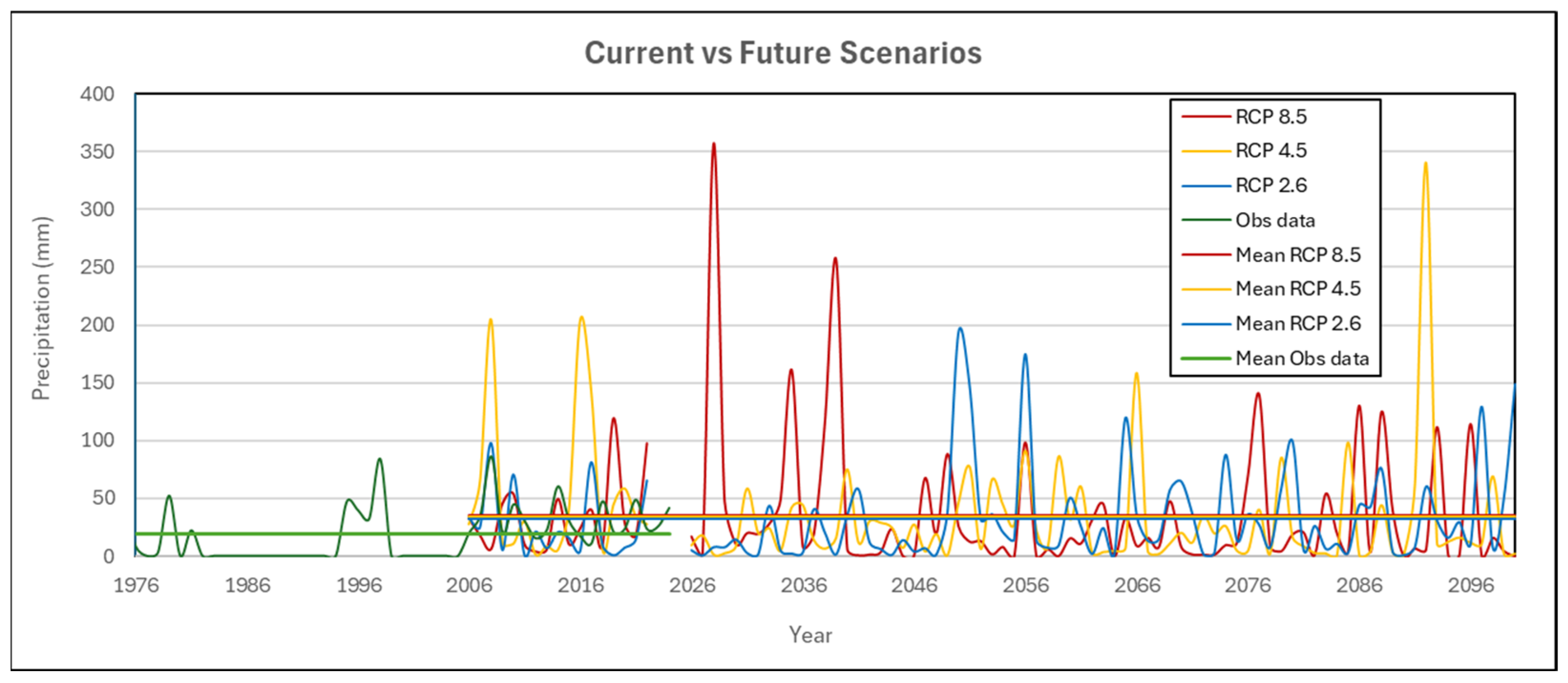
- Under RCP 2.6, the flood volumes increased to 28,793 × 103 m3 (50 years) and 38,927 × 103 m3 (200 years), with the average depths rising to 0.3 m. Under RCP 4.5, the flood volumes nearly doubled, reaching 33,407 × 103 m3 (50 years) and 64,947 × 103 m3 (200 years), while the average depths increased from 0.3 m to 0.6 m. The most extreme increases were projected under RCP 8.5, with the flood volumes peaking at 86,061 × 103 m3 (200 years) and the depths reaching 0.8 m.
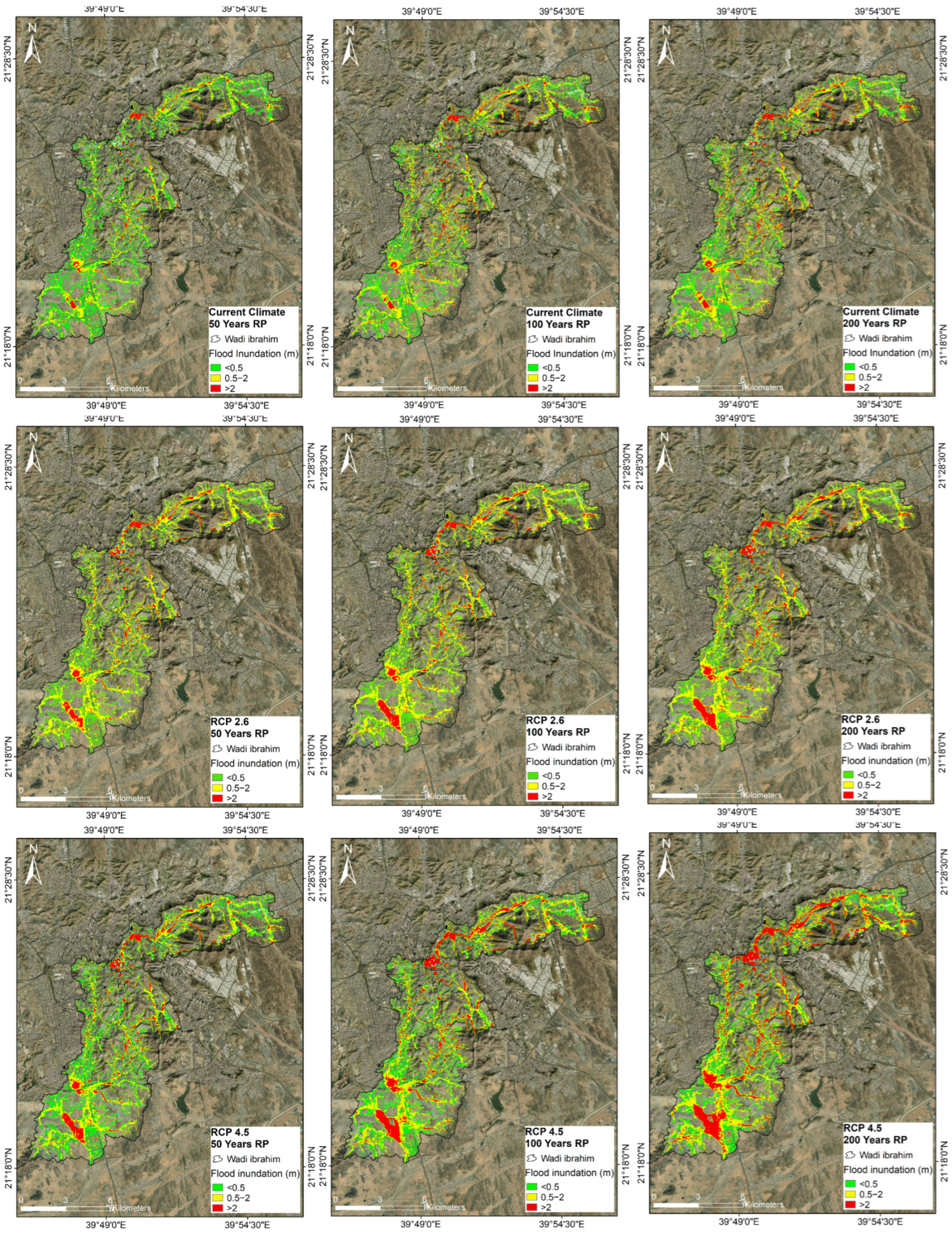
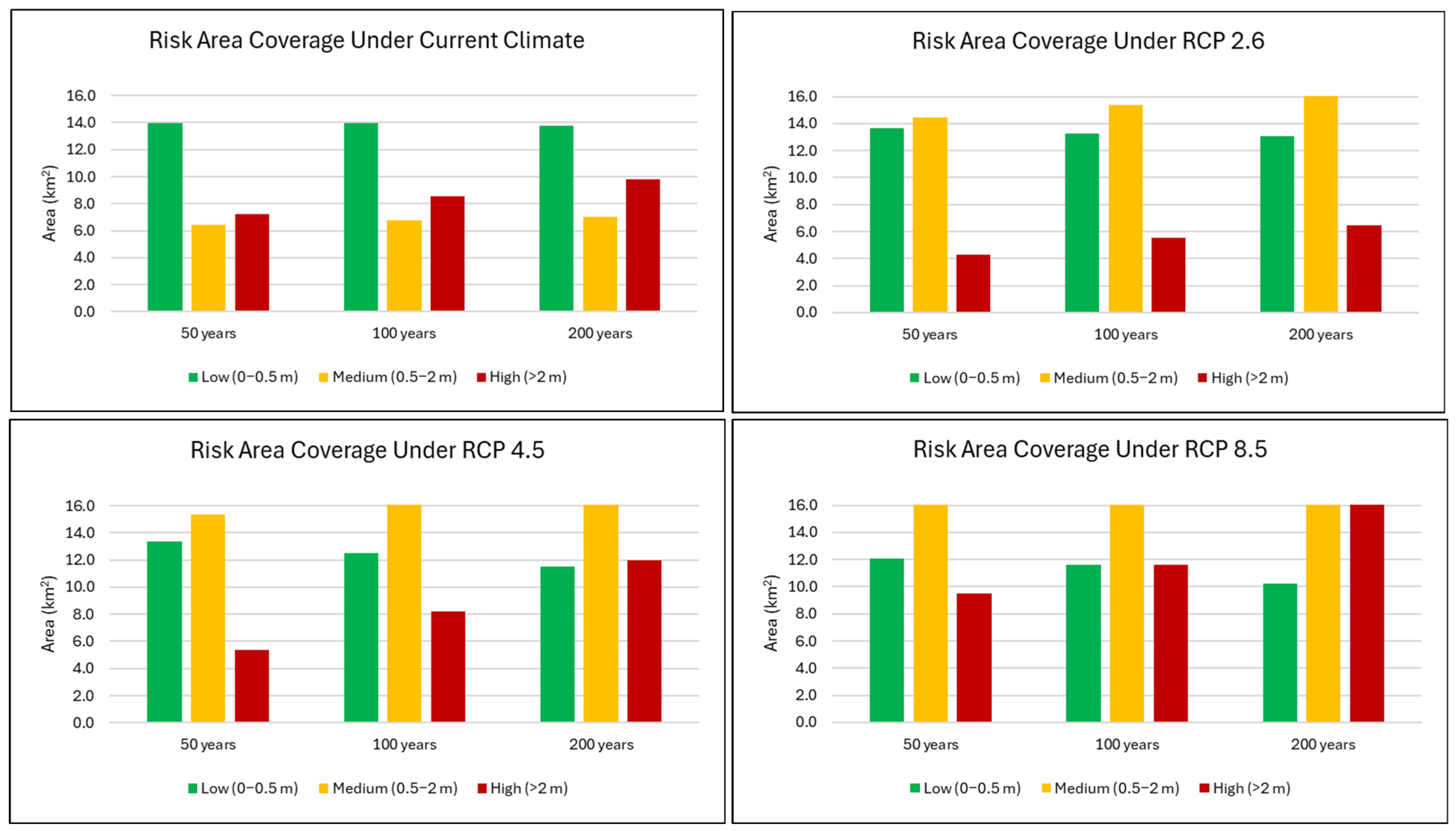
- Flood risk mapping indicated a significant expansion of the medium- and high-risk zones. Under current climate conditions, the low-risk areas (0–0.5 m) decreased slightly from 13.9 km2 (50-year) to 13.8 km2 (200-year); the medium-risk areas (0.5–2 m) expanded from 6.5 km2 to 7.0 km2; and the high-risk areas (>2 m) increased from 7.2 km2 to 9.8 km2.
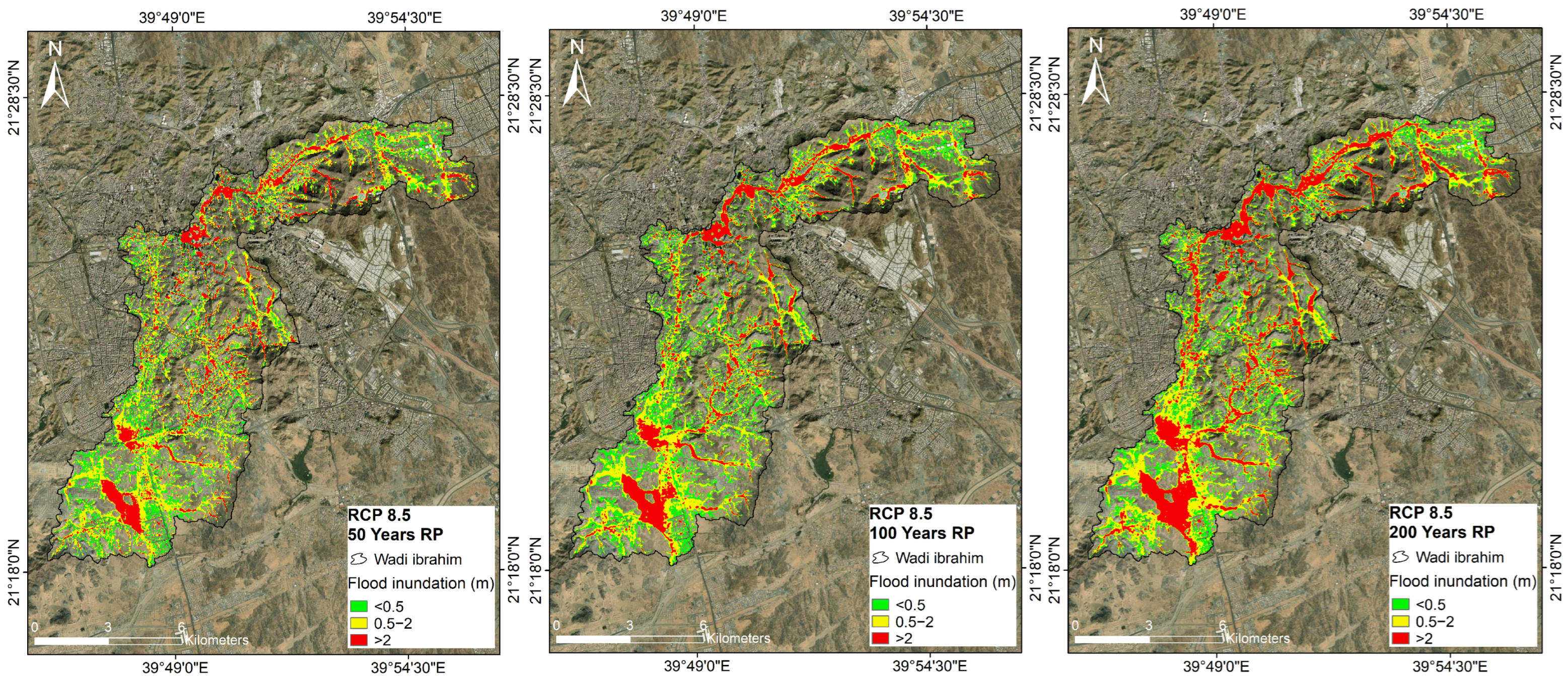
- Under RCP 2.6, the high-risk areas increased from 4.3 km2 (50 years) to 6.5 km2 (200 years); under RCP 4.5, from 5.3 km2 to 12.0 km2; and under RCP 8.5, from 9.5 km2 to 16.6 km2.
- The projected increases in the peak discharge and runoff volume under future climate scenarios underscore the escalating flood risks, especially for higher return periods.
Author Contributions
Funding
Data Availability Statement
Conflicts of Interest
References
- World Meteorological Organization. In the Wake of a Looming Water Crisis, Report Warns. Available online: https://wmo.int/news/media-centre/wake-looming-water-crisis-report-warns (accessed on 8 May 2025).
- UNESCO. United Nations World Water Development Report. Available online: https://www.unesco.org/reports/wwdr/2023/en (accessed on 8 May 2025).
- Kellens, W.; Terpstra, T.; De Maeyer, P. Perception and communication of flood risks: A systematic review of empirical research. Risk Anal. Int. J. 2013, 33, 24–49. [Google Scholar] [CrossRef] [PubMed]
- Jongman, B.; Ward, P.J.; Aerts, J.C. Global exposure to river and coastal flooding: Long term trends and changes. Glob. Environ. Change 2012, 22, 823–835. [Google Scholar] [CrossRef]
- Em-dat, C. The OFDA/CRED International Disaster Database; Université Catholique: Lille, France, 2010. [Google Scholar]
- Subyani, A.M. Hydrologic behavior and flood probability for selected arid basins in Makkah area, western Saudi Arabia. Arab. J. Geosci. 2011, 4, 817. [Google Scholar] [CrossRef]
- Hudson, P.; Botzen, W.W.; Aerts, J.C. Flood insurance arrangements in the European Union for future flood risk under climate and socioeconomic change. Glob. Environ. Change 2019, 58, 101966. [Google Scholar] [CrossRef]
- Wasko, C.; Nathan, R.; Stein, L.; O’Shea, D. Evidence of shorter more extreme rainfalls and increased flood variability under climate change. J. Hydrol. 2021, 603, 126994. [Google Scholar] [CrossRef]
- Roy, P.; Pal, S.C.; Chakrabortty, R.; Chowdhuri, I.; Saha, A.; Shit, M. Effects of climate change and sea-level rise on coastal habitat: Vulnerability assessment, adaptation strategies and policy recommendations. J. Environ. Manag. 2023, 330, 117187. [Google Scholar] [CrossRef] [PubMed]
- Xiong, J.; Yang, Y. Climate Change and Hydrological Extremes. Curr. Clim. Change Rep. 2024, 11, 1. [Google Scholar] [CrossRef]
- Lan, H.; Zhao, Z.; Li, L.; Li, J.; Fu, B.; Tian, N.; Lai, R.; Zhou, S.; Zhu, Y.; Zhang, F. Climate change drives flooding risk increases in the Yellow River Basin. Geogr. Sustain. 2024, 5, 193–199. [Google Scholar] [CrossRef]
- Chien, H.; Yeh, P.J.-F.; Knouft, J.H. Modeling the potential impacts of climate change on streamflow in agricultural watersheds of the Midwestern United States. J. Hydrol. 2013, 491, 73–88. [Google Scholar] [CrossRef]
- Hiraga, Y.; Tahara, R.; Meza, J. A methodology to estimate Probable Maximum Precipitation (PMP) under climate change using a numerical weather model. J. Hydrol. 2025, 652, 132659. [Google Scholar] [CrossRef]
- Moradian, S.; Gharbia, S.; Torabi Haghighi, A.; Olbert, I.A. Modelling extreme precipitation projections under the effects of climate change: Case study of the Caspian Sea. Int. J. Water Resour. Dev. 2025, 41, 57–77. [Google Scholar] [CrossRef]
- Mishra, B.K.; Rafiei Emam, A.; Masago, Y.; Kumar, P.; Regmi, R.K.; Fukushi, K. Assessment of future flood inundations under climate and land use change scenarios in the Ciliwung River Basin, Jakarta. J. Flood Risk Manag. 2018, 11, S1105–S1115. [Google Scholar] [CrossRef]
- UN-Habitat. Makkah City Profile. Available online: https://unhabitat.org/sites/default/files/2020/03/makkah.pdf (accessed on 20 January 2025).
- Shaaban, F.; Othman, A.; Habeebullah, T.M.; El-Saoud, W.A. An integrated GPR and geoinformatics approach for assessing potential risks of flash floods on high-voltage towers, Makkah, Saudi Arabia. Environ. Earth Sci. 2021, 80, 199. [Google Scholar] [CrossRef]
- El Bastawesy, M.; Al Harbi, K.; Habeebullah, T. The hydrology of Wadi Ibrahim Catchment in Makkah City, the Kingdom of Saudi Arabia: The interplay of urban development and flash flood hazards. Life Sci. J. 2012, 9, 580–589. [Google Scholar]
- Chow, V. Applied Hydrology; McGraw-Hill: New York, NY, USA, 1988. [Google Scholar]
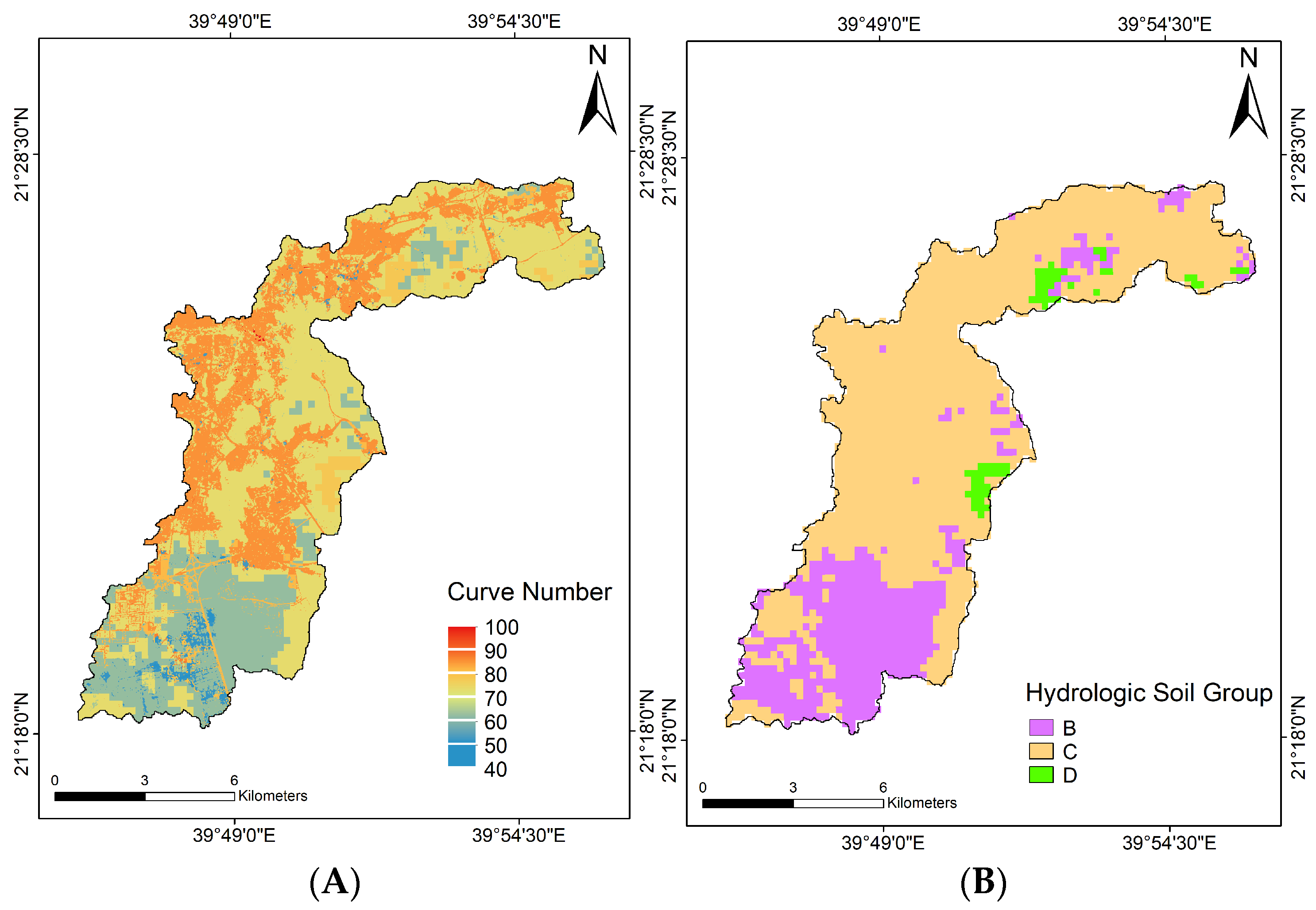
- Siddiqui, A.R. Curve Number Generator: A QGIS Plugin to Generate Curve Number Layer from Land Use and Soil. 2020. Available online: https://github.com/ar-siddiqui/curve_number_generator (accessed on 20 January 2025).
- Ross, C.; Prihodko, L.; Anchang, J.; Kumar, S.; Ji, W.; Hanan, N. Global Hydrologic Soil Groups (HYSOGs250m) for Curve Number-Based Runoff Modeling; ORNL DAAC: Oak Ridge, TN, USA, 2018. [Google Scholar]
- Rathjens, H.; Bieger, K.; Srinivasan, R.; Chaubey, I.; Arnold, J.G.; CMhyd User Manual. Documentation for Preparing Simulated Climate Change Data for Hydrologic Impact Studies. 2016. Available online: http://swat.tamu.edu/software/cmhyd/ (accessed on 10 December 2024).
- Teutschbein, C.; Seibert, J. Bias correction of regional climate model simulations for hydrological climate-change impact studies: Review and evaluation of different methods. J. Hydrol. 2012, 456, 12–29. [Google Scholar] [CrossRef]
- Ewea, H.A.; Elfeki, A.M.; Bahrawi, J.A.; Al-Amri, N.S. Modeling of IDF curves for stormwater design in Makkah Al Mukarramah region, The Kingdom of Saudi Arabia. Open Geosci. 2018, 10, 954–969. [Google Scholar] [CrossRef]
- Kite, G.W. Frequency and Risk Analyses in Hydrology; Water Resources Publications: Littleton, CO, USA, 1977; p. 224. [Google Scholar]
- Ewea, H.A.; Elfeki, A.M.; Al-Amri, N.S. Development of intensity–duration–frequency curves for the Kingdom of Saudi Arabia. Geomat. Nat. Hazards Risk 2017, 8, 570–584. [Google Scholar] [CrossRef]
- Hall, J. Direct rainfall flood modelling: The good, the bad and the ugly. Australas. J. Water Resour. 2015, 19, 74–85. [Google Scholar] [CrossRef]
- Zeiger, S.J.; Hubbart, J.A. Measuring and modeling event-based environmental flows: An assessment of HEC-RAS 2D rain-on-grid simulations. J. Environ. Manag. 2021, 285, 112125. [Google Scholar] [CrossRef]
- Ryan, P.; Syme, B.; Gao, S.; Collecutt, G. Direct rainfall hydraulic model validation. In Proceedings of the Hydrology & Water Resources Symposium 2022 (HWRS 2022): The Past, the Present, the Future: The Past, the Present, the Future, Brisbane, Australia, 30 November–2 December 2022; pp. 421–433. [Google Scholar]
- Utama, R.N.; Ginting, B.M.; Ginting, S. Pemodelan Rain-On-Grid Untuk Kasus Banjir pada Polder Pluit, Jakarta. Rekayasa Sipil 2023, 17, 308–314. [Google Scholar] [CrossRef]
- Kalra, A.; Thakur, B.; Aryal, A.; Gupta, R. A 2D Rain-on-Mesh Model for Simultaneous Hydrologic and Hydraulic Computation. In Proceedings of the World Environmental and Water Resources Congress, Henderson, NC, USA, 21–25 May 2023; pp. 594–606. [Google Scholar]
- Godara, N.; Bruland, O.; Alfredsen, K. Simulation of flash flood peaks in a small and steep catchment using rain-on-grid technique. J. Flood Risk Manag. 2023, 16, e12898. [Google Scholar] [CrossRef]
- Devi, N.N.; Kuiry, S.N. Rain-On-Grid Local-Inertial Formulation to Model Within Grid Topography. In Proceedings of the International Conference on Hydraulics, Water Resources and Coastal Engineering, Chandigarh, India, 22–24 December 2022; pp. 439–449. [Google Scholar]
- Savitri, Y.R.; Kakimoto, R.; Anwar, N.; Wardoyo, W.; Suryani, E. Reliability of 2D hydrodynamic model on flood inundation analysis. Geomate J. 2021, 21, 65–71. [Google Scholar] [CrossRef]
- Ponce, V.M.; Simons, D.B. Shallow wave propagation in open channel flow. J. Hydraul. Div. 1977, 103, 1461–1476. [Google Scholar] [CrossRef]
- Ferrick, M.G.; Bilmes, J.; Long, S.E. Modeling rapidly varied flow in tailwaters. Water Resour. Res. 1984, 20, 271–289. [Google Scholar] [CrossRef]
- Ponce, V.M. Generalized diffusion wave equation with inertial effects. Water Resour. Res. 1990, 26, 1099–1101. [Google Scholar] [CrossRef]
- Tsai, C.W. Applicability of kinematic, noninertia, and quasi-steady dynamic wave models to unsteady flow routing. J. Hydraul. Eng. 2003, 129, 613–627. [Google Scholar] [CrossRef]
- Moramarco, T.; Pandolfo, C.; Singh, V.P. Accuracy of kinematic wave and diffusion wave approximations for flood routing. I: Steady analysis. J. Hydrol. Eng. 2008, 13, 1078–1088. [Google Scholar] [CrossRef]
- Brunner, G.W. HEC-RAS River Analysis System: Hydraulic Reference Manual, Version 5.0; US Army Corps of Engineers, Institute for Water Resources, Hydrologic Engineering Center: Davis, CA, USA, 2010. [Google Scholar]
- Brunner, G.W. HEC-RAS River Analysis System. 2D Modeling User’s Manual, Version 5.0; US Army Corps of Engineers, Institute for Water Resources, Hydrologic Engineering Center: Davis, CA, USA, 2016. [Google Scholar]
- Hazus-Mh, F. FEMA’s Methodology for Estimating Potential Losses from Disasters; US Federal Emergency Management Agency: Hyattsville, MD, USA, 2004. [Google Scholar]
- Abdulrazzak, M.; Elfeki, A.; Kamis, A.; Kassab, M.; Alamri, N.; Chaabani, A.; Noor, K. Flash flood risk assessment in urban arid environment: Case study of Taibah and Islamic universities’ campuses, Medina, Kingdom of Saudi Arabia. Geomat. Nat. Hazards and Risk 2019, 10, 780–796. [Google Scholar] [CrossRef]
- Francou, J.; Rodier, J. Essai de Classification des Crues Maximales. 1969. Available online: https://agris.fao.org/search/en/providers/122415/records/647368e853aa8c89630d79c7 (accessed on 1 January 2025).
- Hidayatulloh, A.; Chaabani, A.; Zhang, L.; Elhag, M. DEM study on hydrological response in Makkah City, Saudi Arabia. Sustainability 2022, 14, 13369. [Google Scholar] [CrossRef]
- Almazroui, M.; Saeed, S.; Islam, M.N.; Khalid, M.S.; Alkhalaf, A.K.; Dambul, R. Assessment of uncertainties in projected temperature and precipitation over the Arabian Peninsula: A comparison between different categories of CMIP3 models. Earth Syst. Environ. 2017, 1, 23. [Google Scholar] [CrossRef]


| Basin Parameters | Ibrahim Watershed |
|---|---|
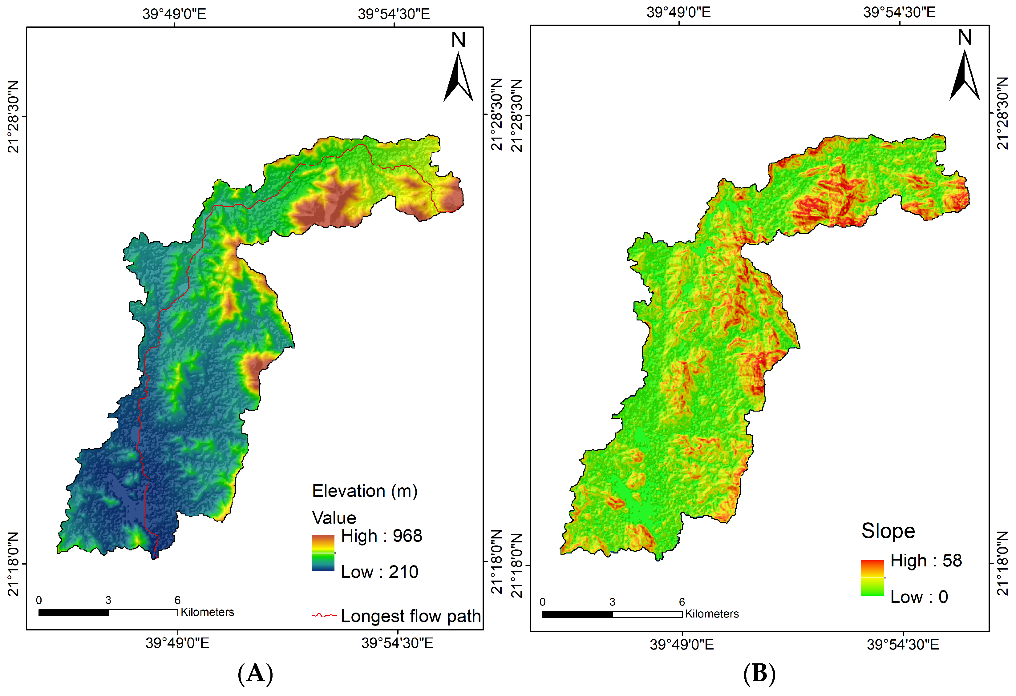
| Low Elevation (m) | 210 |
| High Elevation (m) | 968 |
| Area (km2) | 110.8 |
| Perimeter (km). | 107.2 |
| Longest flow path (km) | 34.6 |
| Basin Length (km) | 28.6 |
| Domain | Middle East and North Africa |
|---|---|
| Experiment | RCP 2.6, RCP 4.5, and RCP 8.5 |
| Horizontal resolution | 0.44 degree × 0.44 degree |
| Temporal resolution | Daily mean |
| Variable | Mean precipitation flux |
| Global climate model | NOAA-GFDL-ESM2M (USA) |
| Regional climate model | SMHI-RCA4 (Sweden) |
| Ensemble member. | r1i1p1 |
| Start year | 2006 |
| End year | 2100 |
| Coordinates | Rainfall (mm) at Different Return Periods (Years) | |||||
|---|---|---|---|---|---|---|
| Scenarios | Stations | Long (E) | Lat (N) | 50 | 100 | 200 |
| Al Adel | 39.85 | 21.44 | 84.70 | 94.80 | 105.00 | |
| Mena | 39.87 | 21.43 | 77.90 | 87.50 | 97.00 | |
| Al Maesem | 39.92 | 21.46 | 59.71 | 66.47 | 73.19 | |
| Electricity | 39.88 | 21.46 | 88.36 | 99.42 | 110.45 | |
| J114 | 39.83 | 21.44 | 97.19 | 110.56 | 123.89 | |
| M139 | 39.82 | 21.41 | 98.64 | 113.55 | 128.41 | |
| Current | Average | 94.51 | 107.09 | 119.62 | ||
| RCP 2.6 | 141.72 | 164.58 | 187.35 | |||
| RCP 4.5 | 150.50 | 175.90 | 201.10 | |||
| RCP 8.5 | 184.30 | 215.80 | 247.30 | |||
 | Extent of Consequences |  | ||||
 Probability of occurrence  | <0.1 m | 0.1–0.5 m | 0.5–1 m | 1–2 m | >2 m | |
| Low | Minor | Major | Severe | Catastrophic | ||
| Possible (1 in 50 years) | High Risk | |||||
| Unlikely (1 in 100 years) | Low Risk | Medium Risk | ||||
| Rare (1 in 200 years) | ||||||
| Current Climate | RCP 26 | RCP 45 | RCP 85 | |||||||||
|---|---|---|---|---|---|---|---|---|---|---|---|---|
| Parameters | Return Period (Years) | Return Period (Years) | Return Period (Years) | Return Period (Years) | ||||||||
| 50 | 100 | 200 | 50 | 100 | 200 | 50 | 100 | 200 | 50 | 100 | 200 | |
| Flood vol (1000 m3) | 18,919 | 21,845 | 24,821 | 28,793 | 34,091 | 38,927 | 33,407 | 47,572 | 64,947 | 44,528 | 63,583 | 86,061 |
| Max depth (m) | 11.8 | 12.5 | 12.7 | 12.9 | 13.3 | 13.5 | 13.2 | 15.7 | 18.4 | 14.9 | 18.3 | 21.5 |
| Average depth (m) | 0.17 | 0.19 | 0.22 | 0.25 | 0.30 | 0.34 | 0.29 | 0.42 | 0.57 | 0.39 | 0.56 | 0.76 |
| Peak discharge (m3/s) | 583 | 701 | 823 | 1045 | 1283 | 1536 | 1245 | 2032 | 3166 | 1844 | 3111 | 4999 |
| Runoff vol (1000 m3) | 6159 | 7335 | 8533 | 10,701 | 13,000 | 15,327 | 12,655 | 19,829 | 30,014 | 18,129 | 29,524 | 46,428 |
Disclaimer/Publisher’s Note: The statements, opinions and data contained in all publications are solely those of the individual author(s) and contributor(s) and not of MDPI and/or the editor(s). MDPI and/or the editor(s) disclaim responsibility for any injury to people or property resulting from any ideas, methods, instructions or products referred to in the content. |
© 2025 by the authors. Licensee MDPI, Basel, Switzerland. This article is an open access article distributed under the terms and conditions of the Creative Commons Attribution (CC BY) license (https://creativecommons.org/licenses/by/4.0/).
Share and Cite
Hidayatulloh, A.; Bahrawi, J. Flood Risk Assessment Under Climate Change Scenarios in the Wadi Ibrahim Watershed. Hydrology 2025, 12, 120. https://doi.org/10.3390/hydrology12050120
Hidayatulloh A, Bahrawi J. Flood Risk Assessment Under Climate Change Scenarios in the Wadi Ibrahim Watershed. Hydrology. 2025; 12(5):120. https://doi.org/10.3390/hydrology12050120
Chicago/Turabian StyleHidayatulloh, Asep, and Jarbou Bahrawi. 2025. "Flood Risk Assessment Under Climate Change Scenarios in the Wadi Ibrahim Watershed" Hydrology 12, no. 5: 120. https://doi.org/10.3390/hydrology12050120
APA StyleHidayatulloh, A., & Bahrawi, J. (2025). Flood Risk Assessment Under Climate Change Scenarios in the Wadi Ibrahim Watershed. Hydrology, 12(5), 120. https://doi.org/10.3390/hydrology12050120