
A New Custom Deep Learning Model Coupled with a Flood Index for Multi-Step-Ahead Flood Forecasting


Abstract
1. Introduction
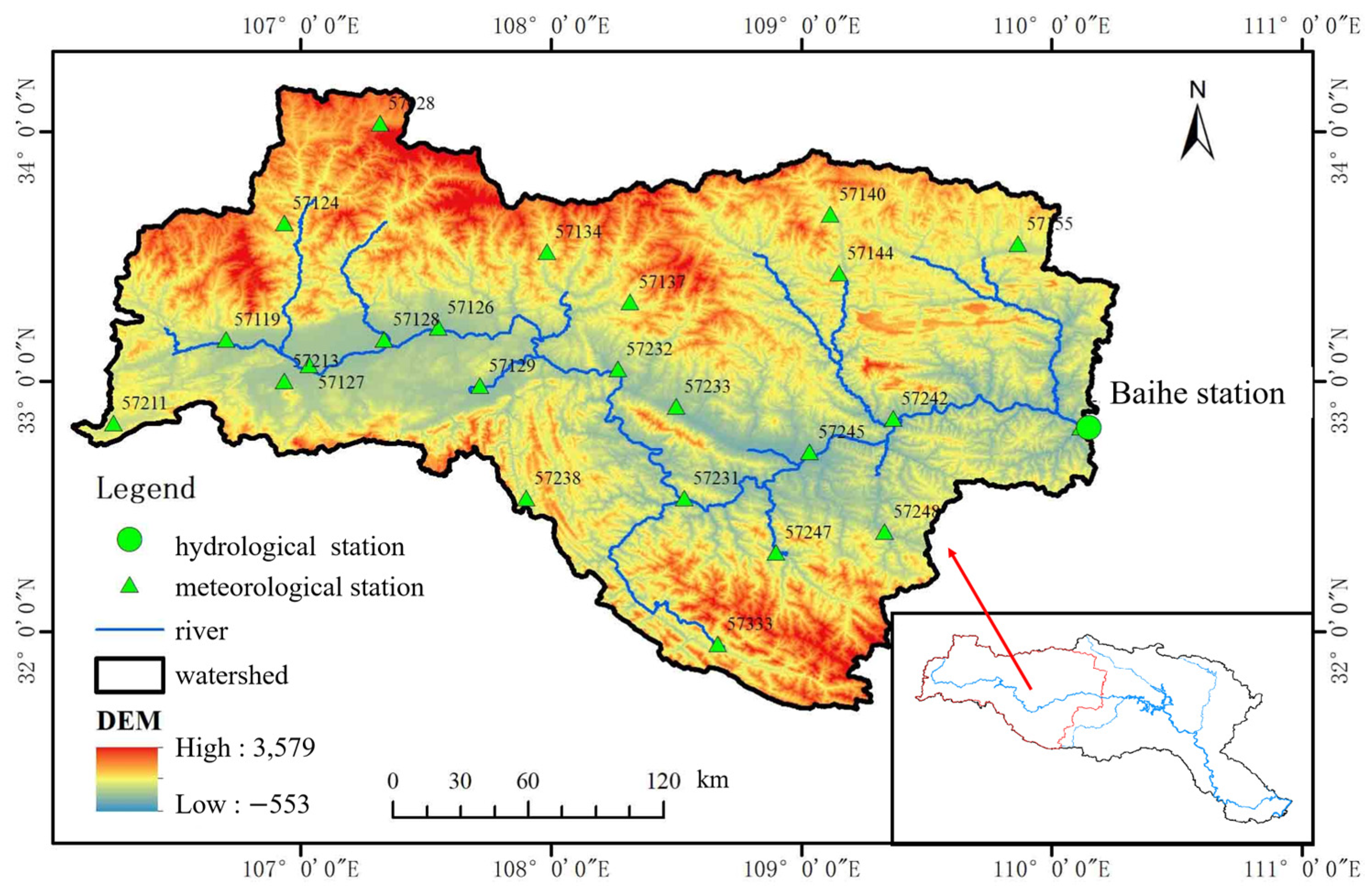
2. Study Area and Data Acquisition
3. Methodology
3.1. Basic Neural Network
3.1.1. Convolutional Neural Network (CNN)
- Input layer: This layer receives structured data (e.g., vectors or matrices) while preserving inherent spatial or temporal relationships.
- Convolutional layer: This layer extracts local features through sliding kernels with shared weights, where more kernels can capture increasingly abstract representations.
- Pooling layer: This layer reduces the spatial dimensions of the feature maps (e.g., via max or average pooling), thereby lowering the computational complexity and mitigating overfitting.
- Fully connected layer: This layer flattens the extracted features into 1D vectors for classification.
- Output layer: This layer generates the final prediction outputs (e.g., class probabilities).
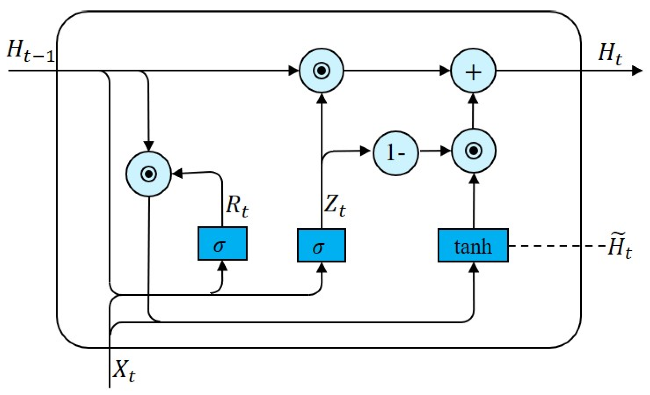
3.1.2. Gated Recurrent Neural Network (GRU)
3.2. Flood Index ()
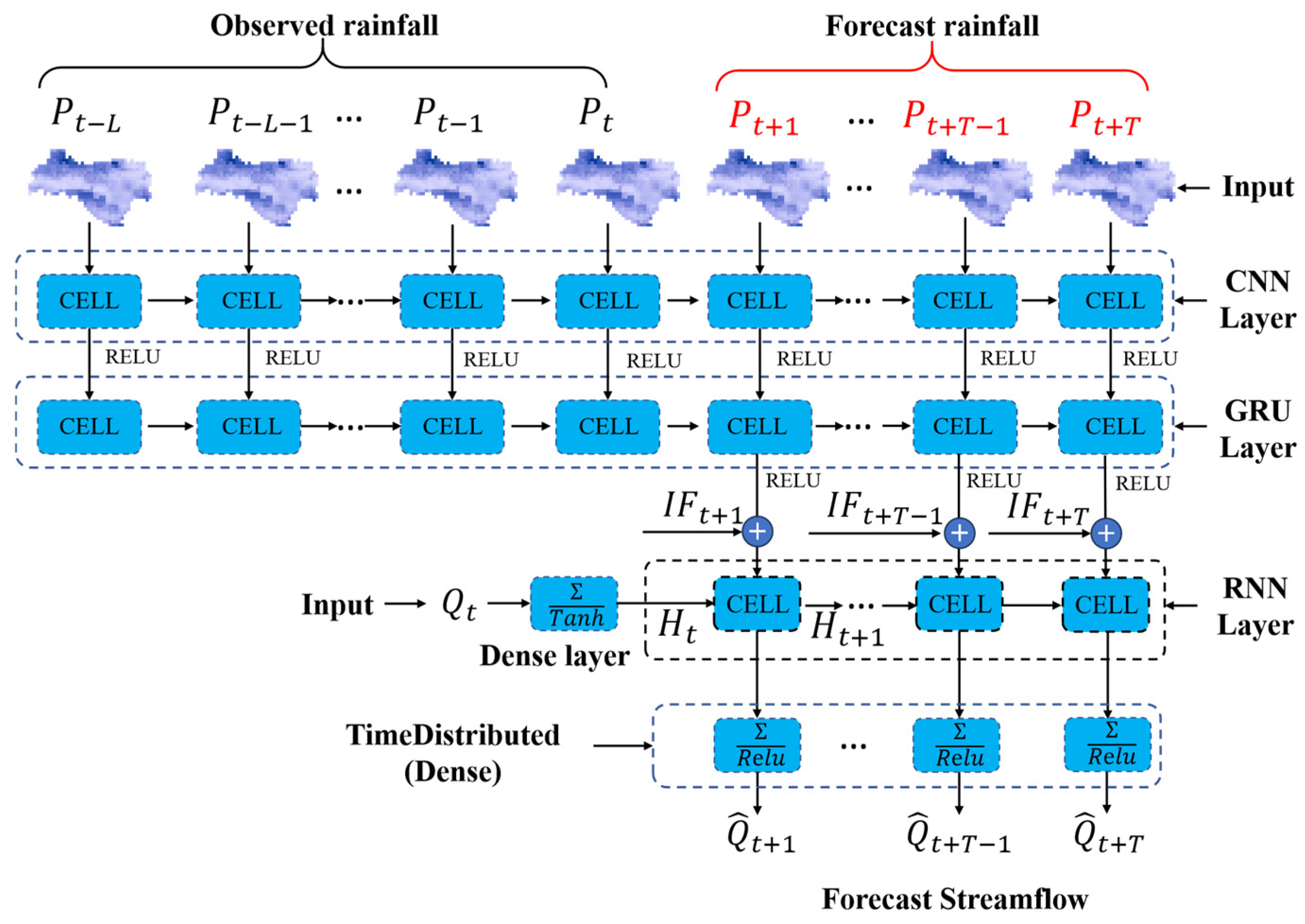
3.3. Proposed Model
3.4. Uncertainty Analysis Method
3.4.1. Comparative Model Structure Design
3.4.2. Subsampling Approach
3.5. Evaluation Metrics
4. Results and Discussion
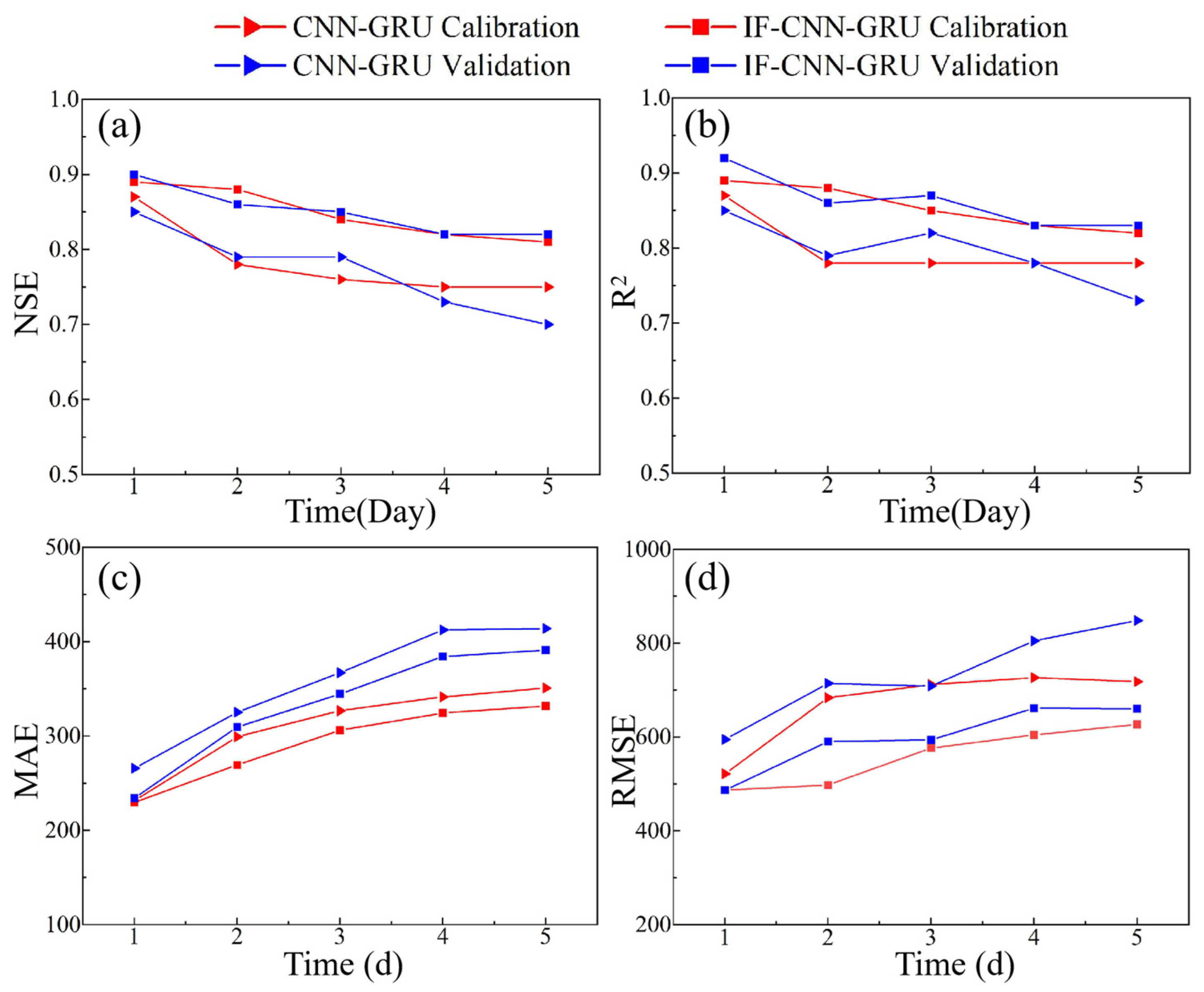
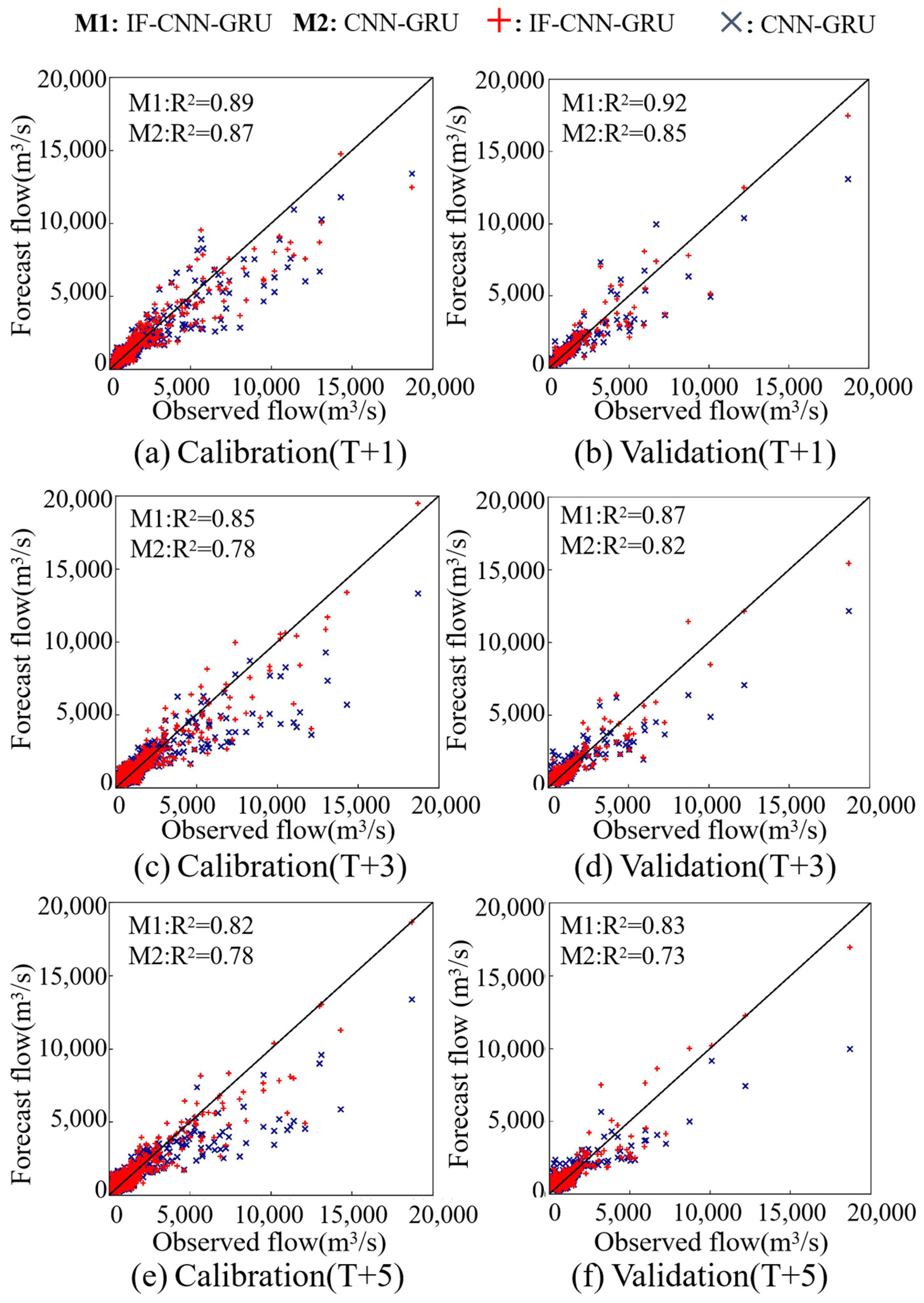
4.1. Performance Assessment
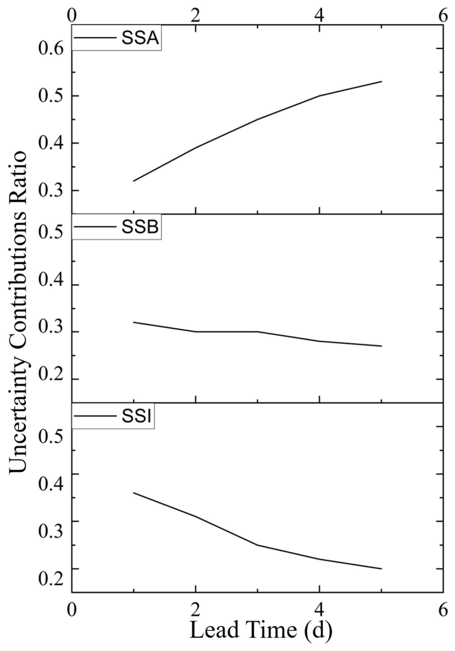
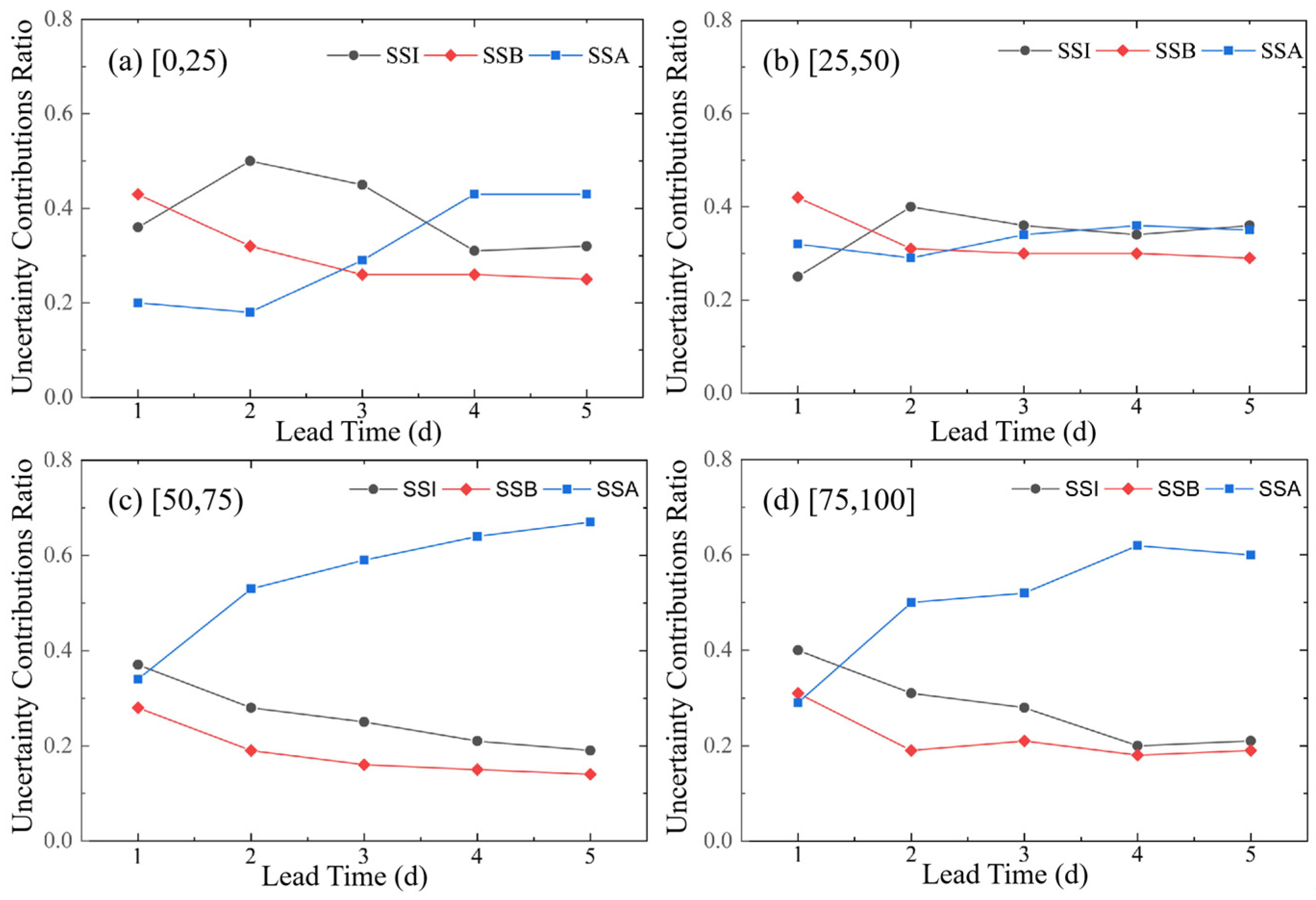
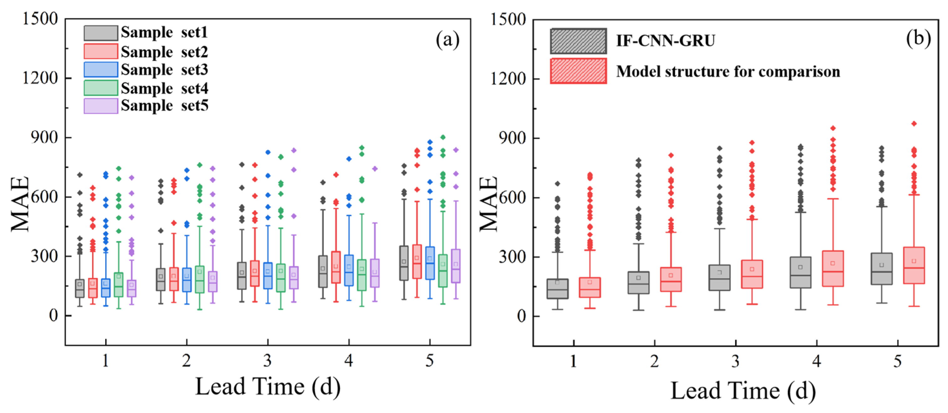
4.2. Uncertainty Source Quantification
5. Conclusions
- (1)
- Incorporating the flood index () enhanced the memory capacity of the RNN by efficiently storing flood information in its state variables, enabling the deep learning-based flood forecast model to extend the forecast period and improving the prediction accuracy.
- (2)
- The uncertainty analysis revealed that the influences of individual modeling factors on the flood forecast uncertainty varied with the forecast period, and the contribution of interactions to the uncertainty was significant. As the forecast period increased, the uncertainty arising from the model inputs gradually increased, whereas the proportion attributable to the model structure decreased.
Author Contributions
Funding
Data Availability Statement
Conflicts of Interest
References
- Khosravi, K.; Pham, B.T.; Chapi, K.; Shirzadi, A.; Shahabi, H.; Revhaug, I.; Prakash, I.; Tien Bui, D. A comparative assessment of decision trees algorithms for flash flood susceptibility modeling at Haraz watershed, northern Iran. Sci. Total Environ. 2018, 627, 744–755. [Google Scholar] [CrossRef] [PubMed]
- Hwang, S.; Yoon, J.; Kang, N.; Lee, D.R. Development of flood forecasting system on city·mountains·small river area in Korea and assessment of forecast accuracy. J. Korea Water Resour. Assoc. 2020, 53, 225–226. [Google Scholar]
- Chen, C.; Jiang, J.; Liao, Z.; Zhou, Y.; Wang, H.; Pei, Q. A short-term flood prediction based on spatial deep learning network: A case study for Xi County, China. J. Hydrol. 2022, 607, 127535. [Google Scholar] [CrossRef]
- Abbot, J.; Marohasy, J. Input selection and optimisation for monthly rainfall forecasting in Queensland, Australia, using artificial neural networks. Atmos. Res. 2014, 138, 166–178. [Google Scholar] [CrossRef]
- Mosavi, A.; Ozturk, P.; Chau, K.-w. Flood Prediction Using Machine Learning Models: Literature Review. Water 2018, 10, 1536. [Google Scholar] [CrossRef]
- Mosavi, A.; Rabczuk, T.; Varkonyi-Koczy, A.R. Reviewing the Novel Machine Learning Tools for Materials Design. In Recent Advances in Technology Research and Education; Springer: Cham, Switzerland, 2018; pp. 50–58. [Google Scholar]
- Dineva, A.; Varkonyi-Koczy, A.R.; Tar, J.K. Fuzzy expert system for automatic wavelet shrinkage procedure selection for noise suppression. In Proceedings of the 18th International Conference on Intelligent Engineering Systems, Tihany, Hungary, 3–5 July 2014; pp. 163–168. [Google Scholar]
- Kim, S.; Matsumi, Y.; Pan, S.; Mase, H. A real-time forecast model using artificial neural network for after runner storm surges on the Tottori coast, Japan. Ocean Eng. 2016, 122, 44–53. [Google Scholar] [CrossRef]
- Suykens, J.A.K.; Vandewalle, J. Least Squares Support Vector Machine Classifiers. Neural Process. Lett. 1999, 9, 293–300. [Google Scholar] [CrossRef]
- Taherei Ghazvinei, P.; Hassanpour Darvishi, H.; Mosavi, A.; Yusof, K.B.W.; Alizamir, M.; Shamshirband, S.; Chau, K.W. Sugarcane growth prediction based on meteorological parameters using extreme learning machine and artificial neural network. Eng. Appl. Comput. Fluid Mech. 2018, 12, 738–749. [Google Scholar] [CrossRef]
- Le, X.H.; Ho, H.V.; Lee, G. River streamflow prediction using a deep neural network: A case study on the Red River, Vietnam. Korean J. Agric. Sci. 2019, 46, 843–856. [Google Scholar] [CrossRef]
- Cho, K.; Van Merrienboer, B.; Gulcehre, C.; Bahdanau, D.; Bougares, F.; Schwenk, H.; Bengio, Y. Learning Phrase Representations using RNN Encoder-Decoder for Statistical Machine Translation. Comput. Sci. 2014. [CrossRef]
- Moishin, M.; Deo, R.C.; Prasad, R.; Raj, N.; Abdulla, S. Designing Deep-Based Learning Flood Forecast Model With ConvLSTM Hybrid Algorithm. IEEE Access 2021, 9, 50982–50993. [Google Scholar] [CrossRef]
- Granata, F.; Di Nunno, F.; de Marinis, G. Stacked machine learning algorithms and bidirectional long short-term memory networks for multi-step ahead streamflow forecasting: A comparative study. J. Hydrol. 2022, 613, 128431. [Google Scholar] [CrossRef]
- Cui, Z.; Guo, S.; Zhou, Y.; Wang, J. Exploration of dual-attention mechanism-based deep learning for multi-step-ahead flood probabilistic forecasting. J. Hydrol. 2023, 622, 129688. [Google Scholar] [CrossRef]
- Luo, Y.; Zhou, Y.; Chen, H.; Xiong, L.; Guo, S.; Chang, F.J. Exploring a spatiotemporal hetero graph-based long short-term memory model for multi-step-ahead flood forecasting. J. Hydrol. 2024, 633, 15. [Google Scholar] [CrossRef]
- Barino, F.O.; Silva, V.N.H.; Barbero, A.P.L.; Honório, L.d.M.; Santos, A.B.D. Correlated Time-Series in Multi-Day-Ahead Streamflow Forecasting Using Convolutional Networks. IEEE Access 2022, 8, 215748–215757. [Google Scholar] [CrossRef]
- Cao, Q.; Zhang, H.; Zhu, F.; Hao, Z.; Yuan, F. Multi-step-ahead flood forecasting using an improved BiLSTM-S2S model. J. Flood Risk Manag. 2022, 15, e12827. [Google Scholar] [CrossRef]
- Ghobadi, F.; Kang, D. Multi-Step Ahead Probabilistic Forecasting of Daily Streamflow Using Bayesian Deep Learning: A Multiple Case Study. Water 2022, 14, 3672. [Google Scholar] [CrossRef]
- Lin, K.; Chen, H.; Zhou, Y.; Sheng, S.; Luo, Y.; Guo, S.; Xu, C.Y. Exploring a similarity search-based data-driven framework for multi-step-ahead flood forecasting. Sci. Total Environ. 2023, 891, 164494. [Google Scholar] [CrossRef]
- Rasouli, K.; Hsieh, W.W.; Cannon, A.J. Daily streamflow forecasting by machine learning methods with weather and climate inputs. J. Hydrol. 2012, 414, 284–293. [Google Scholar] [CrossRef]
- de la Fuente, A.; Meruane, V.; Meruane, C. Hydrological Early Warning System Based on a Deep Learning Runoff Model Coupled with a Meteorological Forecast. Water 2019, 11, 1808. [Google Scholar] [CrossRef]
- Du, J.; Kimball, J.; Sheffield, J.; Pan, M.; Wood, E. Satellite Flood Assessment and Forecasts from SMAP and Landsat. In Proceedings of the IEEE International Geoscience and Remote Sensing Symposium, Waikoloa, HI, USA, 26 September–2 October 2020; pp. 6707–6715. [Google Scholar]
- Nosrati, K.; Saravi, M.M.; Shahbazi, A. Investigation of Flood Event Possibility over Iran Using Flood Index. Vaccine 2010, 21, 1958–1964. [Google Scholar]
- Deo, R.C.; Byun, H.-R.; Adamowski, J.F.; Kim, D.-W. A Real-time Flood Monitoring Index Based on Daily Effective Precipitation and its Application to Brisbane and Lockyer Valley Flood Events. Water Resour. Manag. 2015, 29, 4075–4093. [Google Scholar] [CrossRef]
- Deo, R.C.; Adamowski, J.F.; Begum, K.; Salcedo-Sanz, S.; Kim, D.W.; Dayal, K.S.; Byun, H.R. Quantifying flood events in Bangladesh with a daily-step flood monitoring index based on the concept of daily effective precipitation. Theor. Appl. Climatol. 2019, 137, 1201–1215. [Google Scholar] [CrossRef]
- Moishin, M.; Deo, R.C.; Prasad, R.; Raj, N.; Abdulla, S. Development of Flood Monitoring Index for daily flood risk evaluation: Case studies in Fiji. Stoch. Environ. Res. Risk Assess. 2021, 35, 1387–1402. [Google Scholar] [CrossRef]
- Shen, J.; Liu, P.; Xia, J.; Zhao, Y.; Dong, Y. Merging Multisatellite and Gauge Precipitation Based on Geographically Weighted Regression and Long Short-Term Memory Network. Remote Sens. 2022, 14, 3939. [Google Scholar] [CrossRef]
- Wang, Z.; Yan, W.; Oates, T. Time Series Classification from Scratch with Deep Neural Networks: A Strong Baseline. In Proceedings of the 2017 International Joint Conference on Neural Networks (IJCNN), Anchorage, AK, USA, 14–19 May 2017. [Google Scholar] [CrossRef]
- Fang, W.; Zhang, F.; Sheng, V.S.; Ding, Y. SCENT: A New Precipitation Nowcasting Method Based on Sparse Correspondence and Deep Neural Network. Neurocomputing 2021, 448, 10–20. [Google Scholar] [CrossRef]
- Li, X.; Zhuang, W.; Zhang, H. Short-term Power Load Forecasting Based on Gate Recurrent Unit Network and Cloud Computing Platform. In Proceedings of the 4th International Conference on Computer Science Application Engineering, Sanya, China, 20–22 October 2020. [Google Scholar]
- Bosshard, T.; Carambia, M.; Goergen, K.; Kotlarski, S.; Krahe, P.; Zappa, M.; Schär, C. Quantifying uncertainty sources in an ensemble of hydrological climate-impact projections. Water Resour. Res. 2013, 49, 1523–1536. [Google Scholar] [CrossRef]
- Song, T.; Ding, W.; Liu, H.; Wu, J.; Zhou, H.; Chu, J. Uncertainty Quantification in Machine Learning Modeling for Multi-Step Time Series Forecasting: Example of Recurrent Neural Networks in Discharge Simulations. Water 2020, 12, 912. [Google Scholar] [CrossRef]
- Déqué, M.; Rowell, D.P.; Lüthi, D.; Giorgi, F.; Hurk, B.V.D. An intercomparison of regional climate simulations for Europe: Assessing uncertainties in model projections. Clim. Change 2007, 81, 53–70. [Google Scholar] [CrossRef]
- Zhou, Y.; Guo, S.; Xu, C.-Y.; Chang, F.-J.; Yin, J. Improving the Reliability of Probabilistic Multi-Step-Ahead Flood Forecasting by Fusing Unscented Kalman Filter with Recurrent Neural Network. Water 2020, 12, 578. [Google Scholar] [CrossRef]
- Jha, A.; Chandrasekaran, A.; Kim, C.; Ramprasad, R. Impact of dataset uncertainties on machine learning model predictions: The example of polymer glass transition temperatures. Model. Simul. Mater. Sci. Eng. 2019, 27, 024002. [Google Scholar] [CrossRef]
- Rahmati, O.; Choubin, B.; Fathabadi, A.; Coulon, F.; Soltani, E.; Shahabi, H.; Mollaefar, E.; Tiefenbacher, J.; Cipullo, S.; Ahmad, B.B. Predicting uncertainty of machine learning models for modelling nitrate pollution of groundwater using quantile regression and UNEEC methods. Sci. Total Environ. 2019, 688, 855–866. [Google Scholar] [CrossRef] [PubMed]


| Sample Set | Calibration Dataset | Validation Dataset |
|---|---|---|
| sample set 1 | G1, G2, G3, G4 | G5 |
| sample set 2 | G1, G2, G3, G5 | G4 |
| sample set 3 | G1, G2, G4, G5 | G3 |
| sample set 4 | G1, G3, G4, G5 | G2 |
| sample set 5 | G2, G3, G4, G5 | G1 |
| Lead Time (d) | Phase | Model | NSE | R2 | RMSE | MAE | KGE |
|---|---|---|---|---|---|---|---|
| 1 | Calibration | CNN-GRU | 0.87 | 0.87 | 521.75 | 231.49 | 0.88 |
| IF-CNN-GRU | 0.89 | 0.89 | 486.78 | 229.76 | 0.87 | ||
| Validation | CNN-GRU | 0.85 | 0.85 | 594.92 | 265.83 | 0.88 | |
| IF-CNN-GRU | 0.90 | 0.92 | 486.69 | 234.24 | 0.83 | ||
| 2 | Calibration | CNN-GRU | 0.78 | 0.78 | 683.85 | 299.22 | 0.77 |
| IF-CNN-GRU | 0.88 | 0.88 | 497.79 | 269.46 | 0.88 | ||
| Validation | CNN-GRU | 0.79 | 0.79 | 714.46 | 325.23 | 0.80 | |
| IF-CNN-GRU | 0.86 | 0.86 | 590.55 | 309.64 | 0.84 | ||
| 3 | Calibration | CNN-GRU | 0.76 | 0.78 | 711.79 | 326.93 | 0.71 |
| IF-CNN-GRU | 0.84 | 0.85 | 576.35 | 306.27 | 0.82 | ||
| Validation | CNN-GRU | 0.79 | 0.82 | 708.89 | 367.25 | 0.71 | |
| IF-CNN-GRU | 0.85 | 0.87 | 593.80 | 344.70 | 0.80 | ||
| 4 | Calibration | CNN-GRU | 0.75 | 0.78 | 726.57 | 341.59 | 0.69 |
| IF-CNN-GRU | 0.82 | 0.83 | 604.63 | 324.52 | 0.83 | ||
| Validation | CNN-GRU | 0.73 | 0.78 | 805.12 | 412.43 | 0.66 | |
| IF-CNN-GRU | 0.82 | 0.83 | 661.66 | 384.30 | 0.80 | ||
| 5 | Calibration | CNN-GRU | 0.75 | 0.78 | 718.20 | 350.96 | 0.69 |
| IF-CNN-GRU | 0.81 | 0.82 | 626.89 | 331.97 | 0.78 | ||
| Validation | CNN-GRU | 0.70 | 0.73 | 848.24 | 414.02 | 0.66 | |
| IF-CNN-GRU | 0.82 | 0.83 | 660.19 | 391.05 | 0.78 |
Disclaimer/Publisher’s Note: The statements, opinions and data contained in all publications are solely those of the individual author(s) and contributor(s) and not of MDPI and/or the editor(s). MDPI and/or the editor(s) disclaim responsibility for any injury to people or property resulting from any ideas, methods, instructions or products referred to in the content. |
© 2025 by the authors. Licensee MDPI, Basel, Switzerland. This article is an open access article distributed under the terms and conditions of the Creative Commons Attribution (CC BY) license (https://creativecommons.org/licenses/by/4.0/).
Share and Cite
Shen, J.; Yang, M.; Zhang, J.; Chen, N.; Li, B. A New Custom Deep Learning Model Coupled with a Flood Index for Multi-Step-Ahead Flood Forecasting. Hydrology 2025, 12, 104. https://doi.org/10.3390/hydrology12050104
Shen J, Yang M, Zhang J, Chen N, Li B. A New Custom Deep Learning Model Coupled with a Flood Index for Multi-Step-Ahead Flood Forecasting. Hydrology. 2025; 12(5):104. https://doi.org/10.3390/hydrology12050104
Chicago/Turabian StyleShen, Jianming, Moyuan Yang, Juan Zhang, Nan Chen, and Binghua Li. 2025. "A New Custom Deep Learning Model Coupled with a Flood Index for Multi-Step-Ahead Flood Forecasting" Hydrology 12, no. 5: 104. https://doi.org/10.3390/hydrology12050104
APA StyleShen, J., Yang, M., Zhang, J., Chen, N., & Li, B. (2025). A New Custom Deep Learning Model Coupled with a Flood Index for Multi-Step-Ahead Flood Forecasting. Hydrology, 12(5), 104. https://doi.org/10.3390/hydrology12050104