
Assessing Deep Learning Techniques for Remote Gauging and Water Quality Monitoring Using Webcam Images


Abstract
1. Introduction
2. Methods
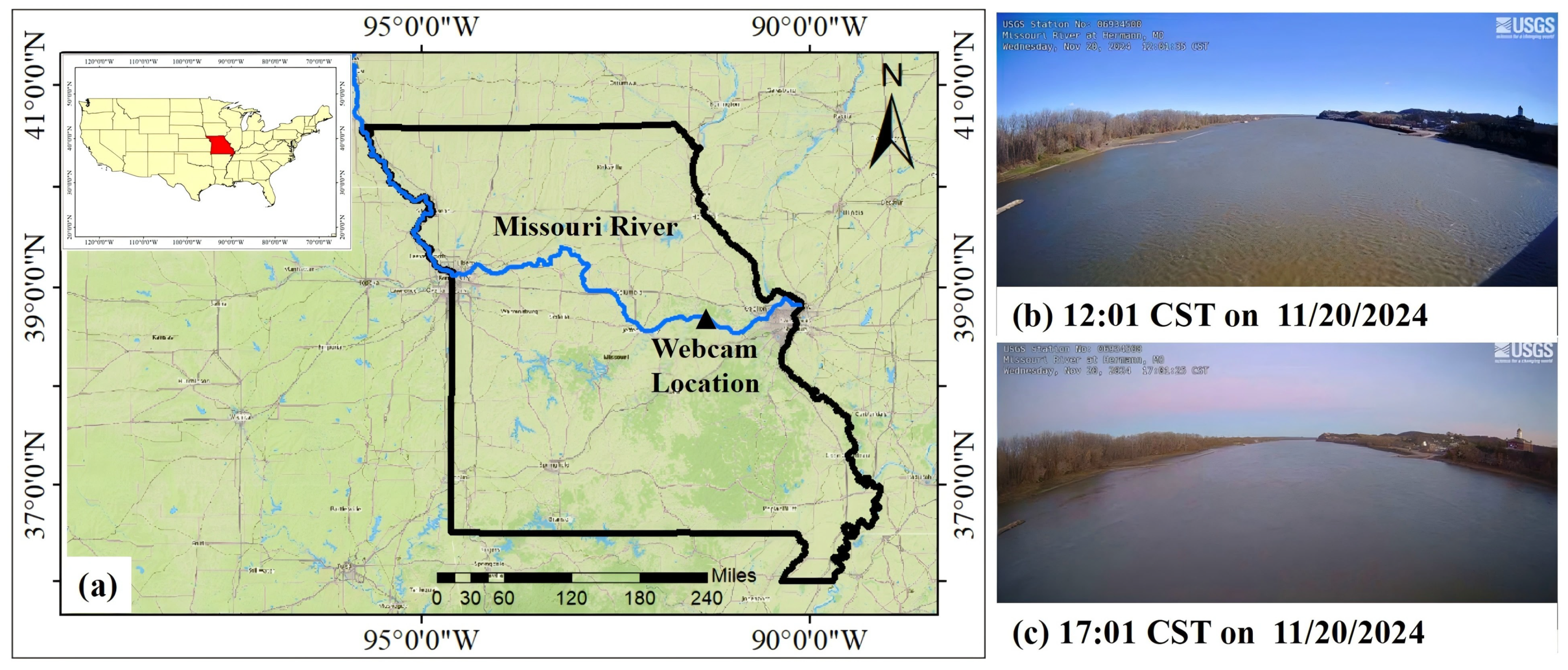
2.1. Image Data
2.2. Gauging Data
2.3. CNN-Based Architectures
2.4. Model Training, Validation, and Deployment
3. Results and Discussion
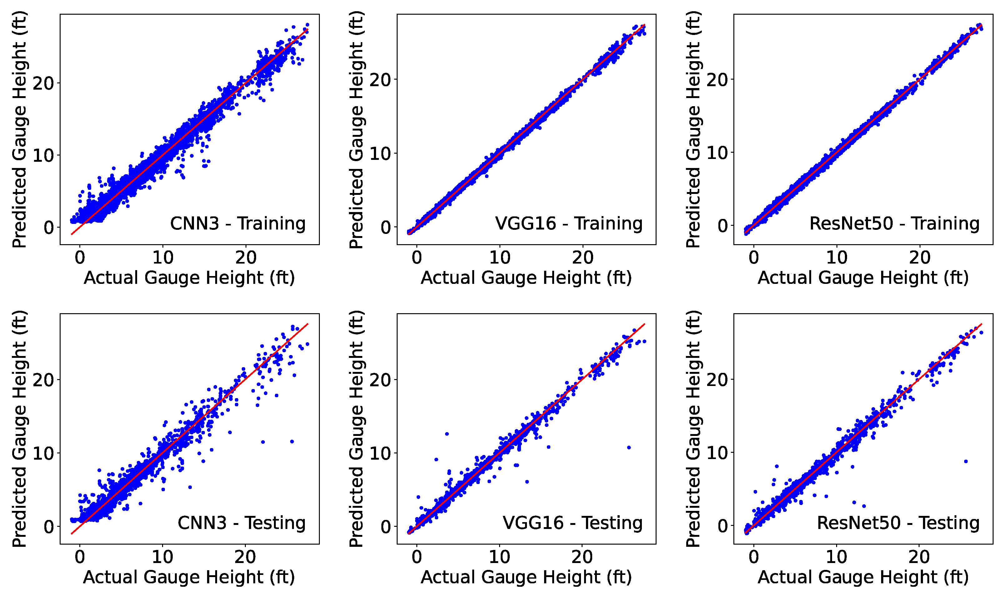
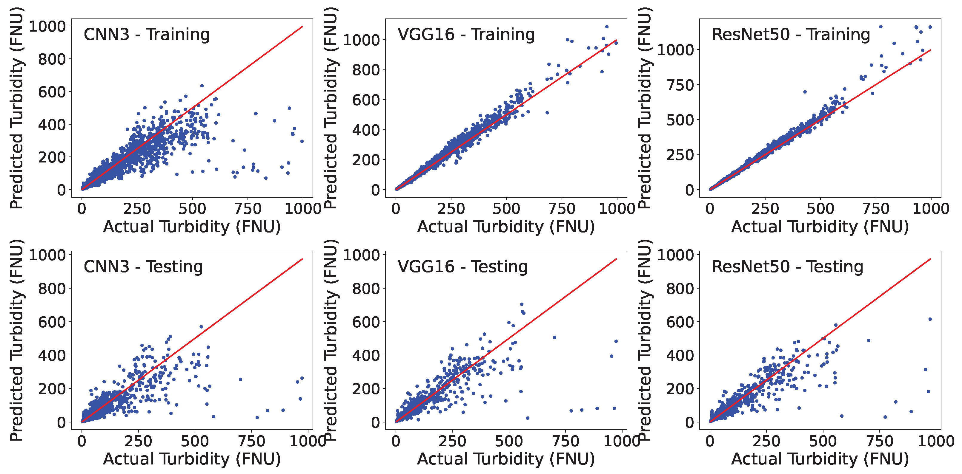
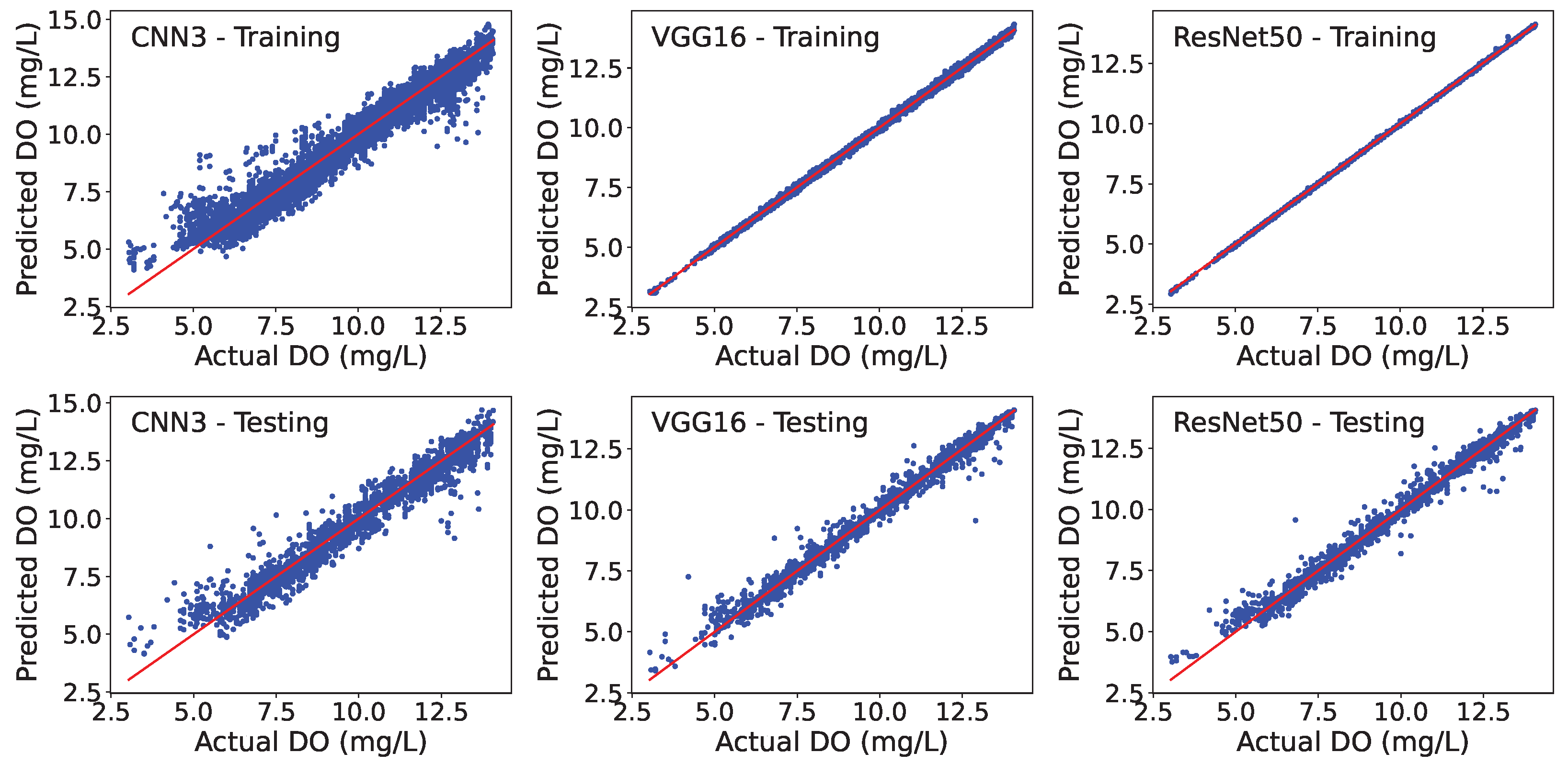
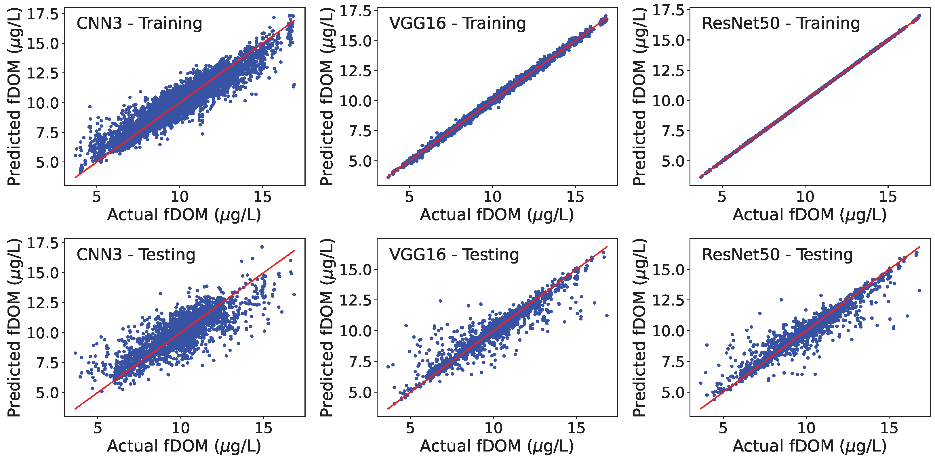
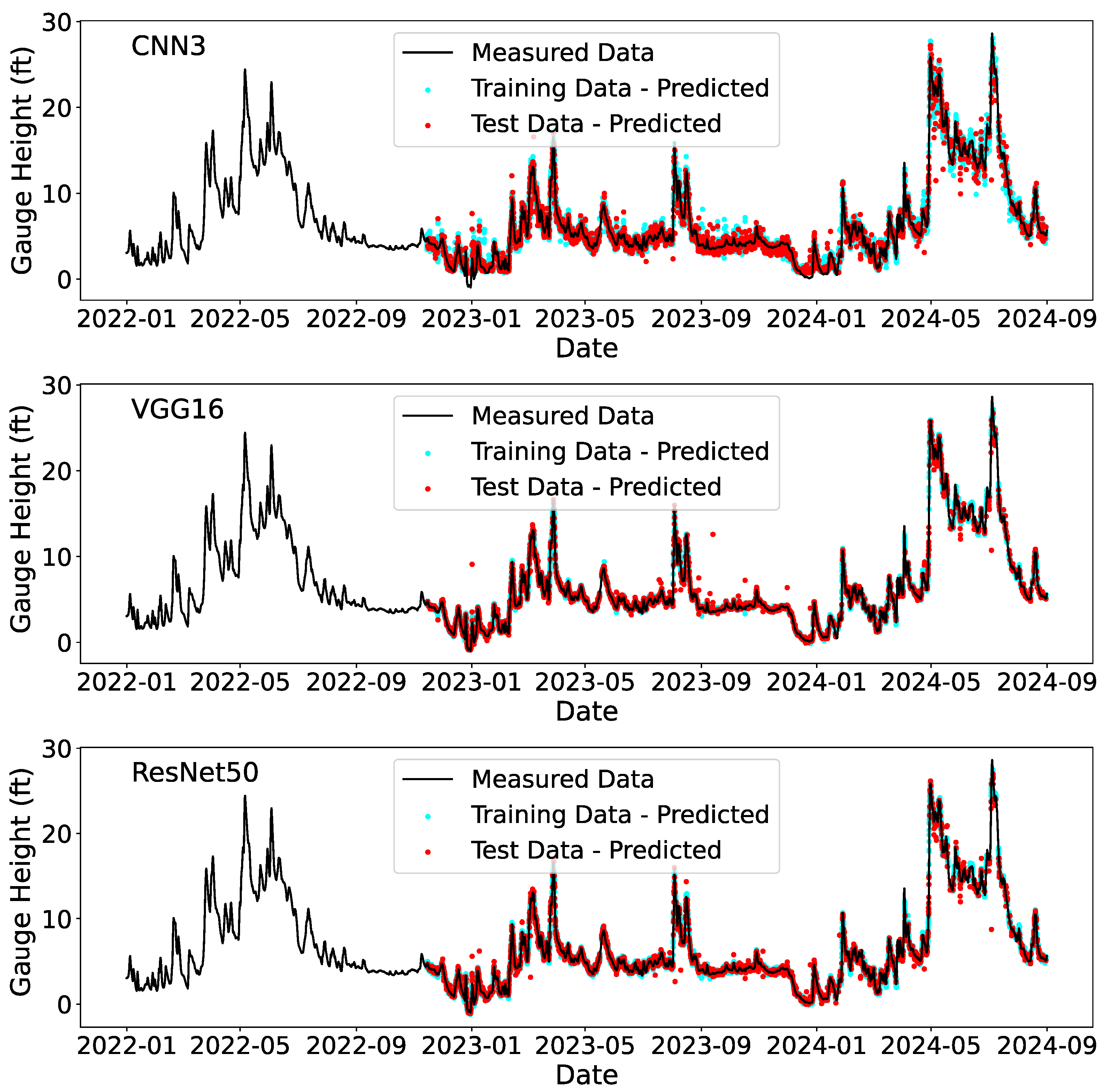
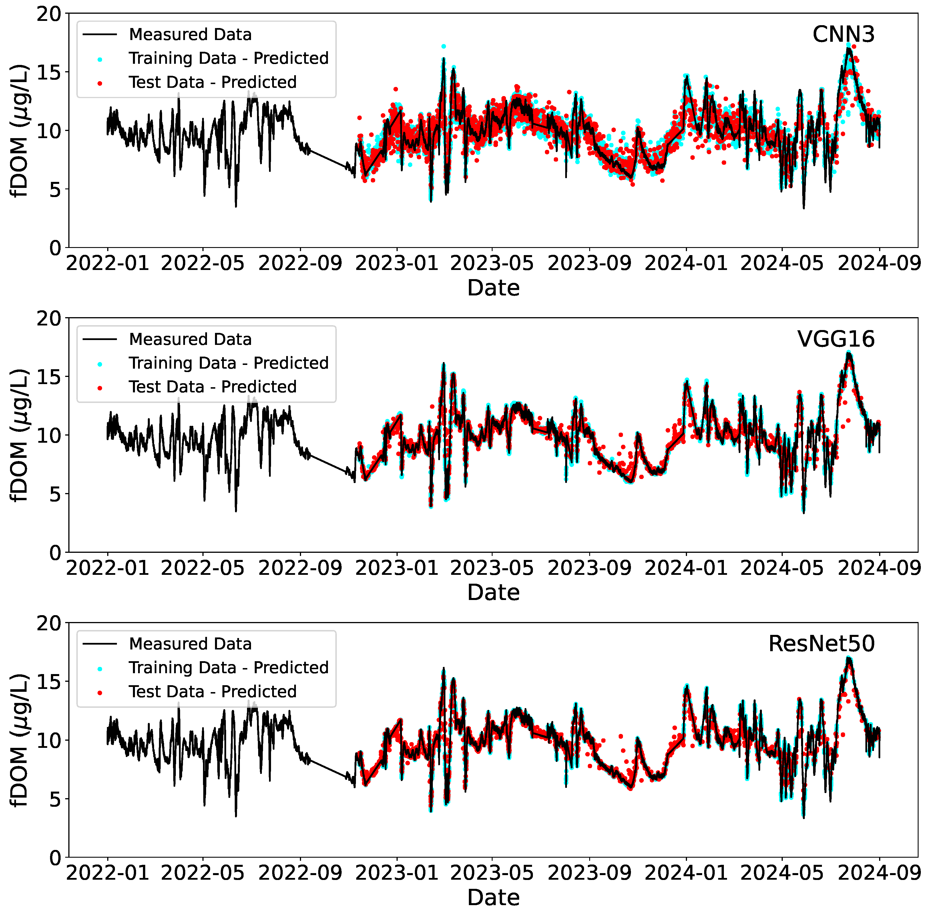
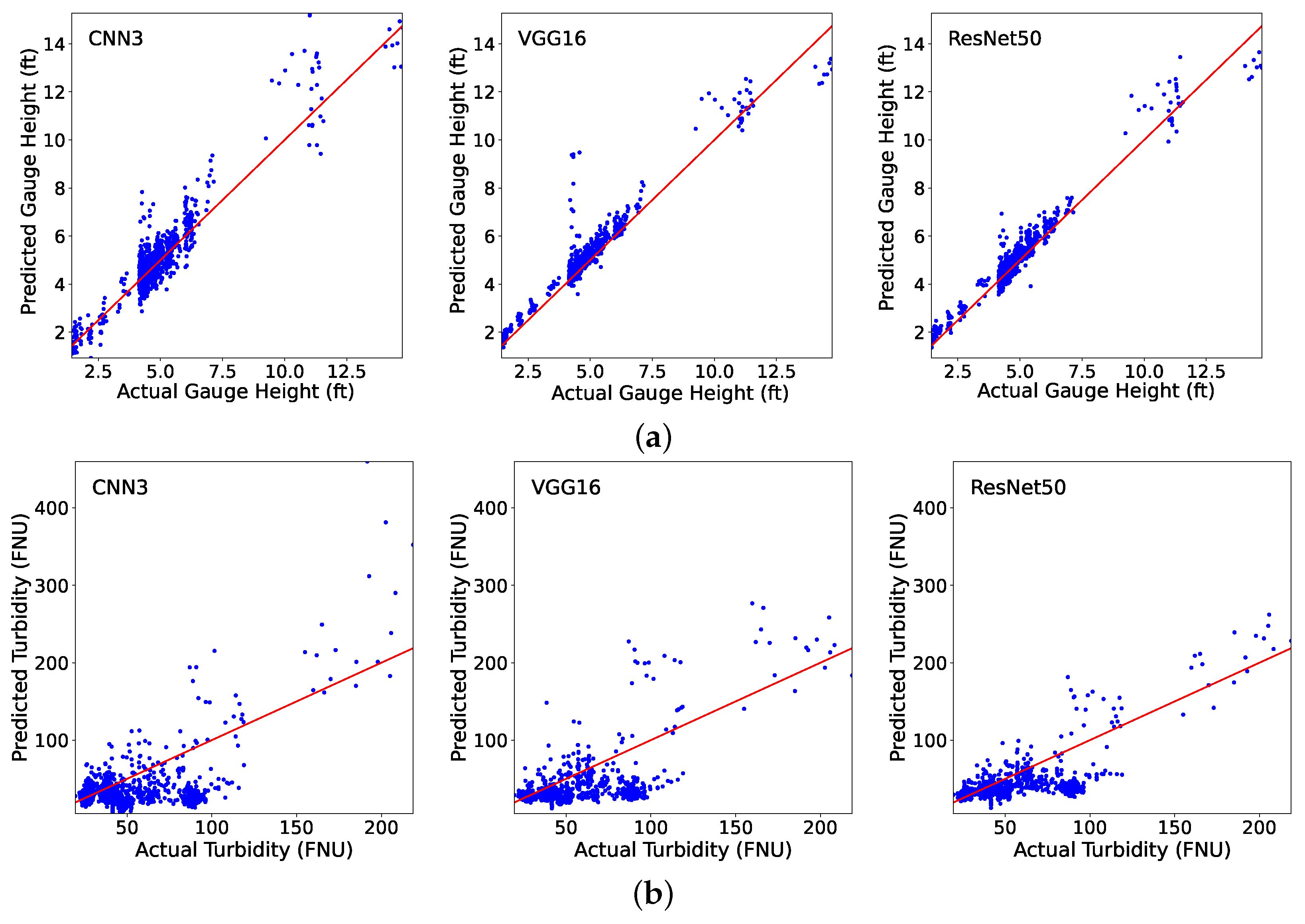
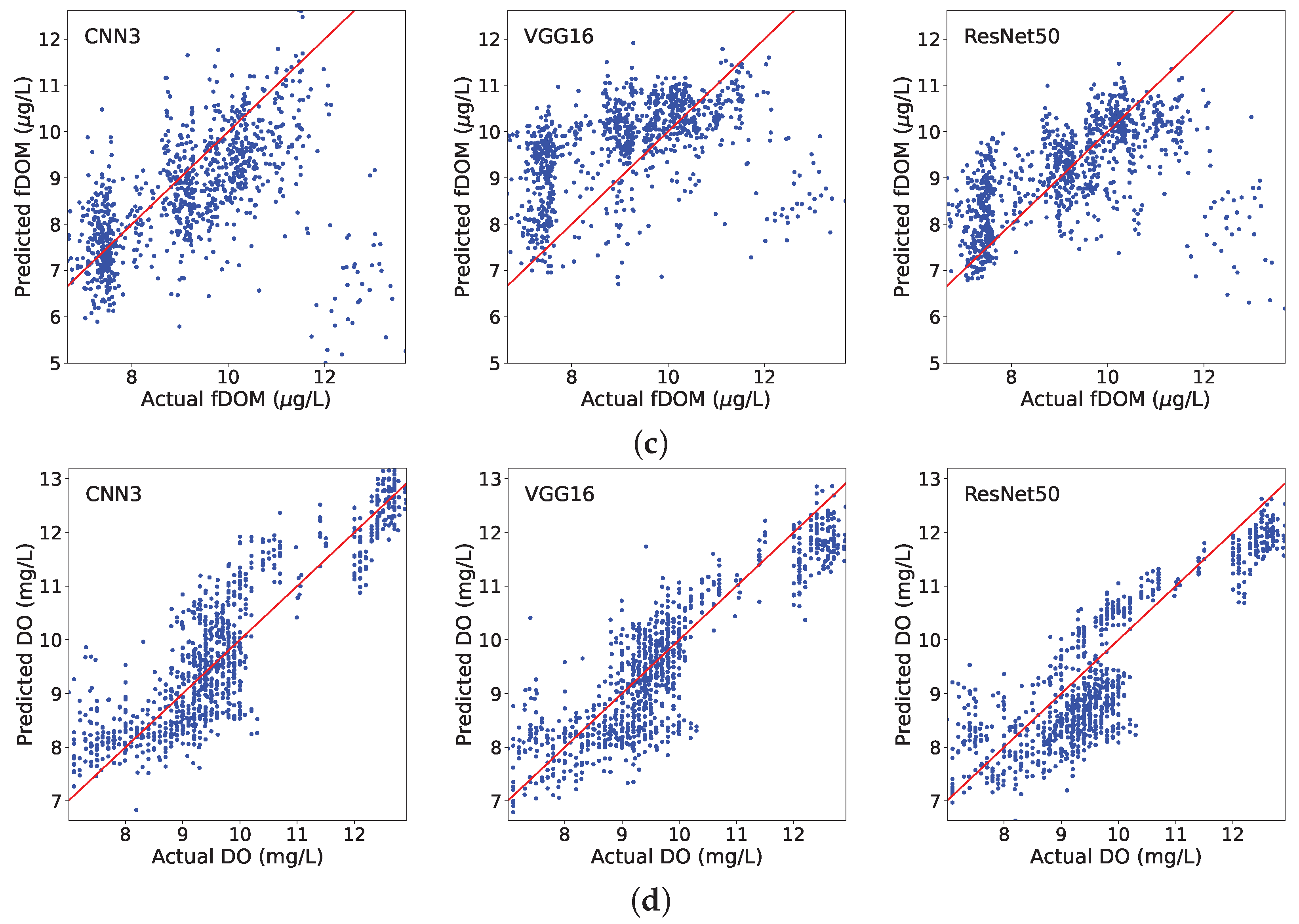
3.1. Modeling Training and Testing
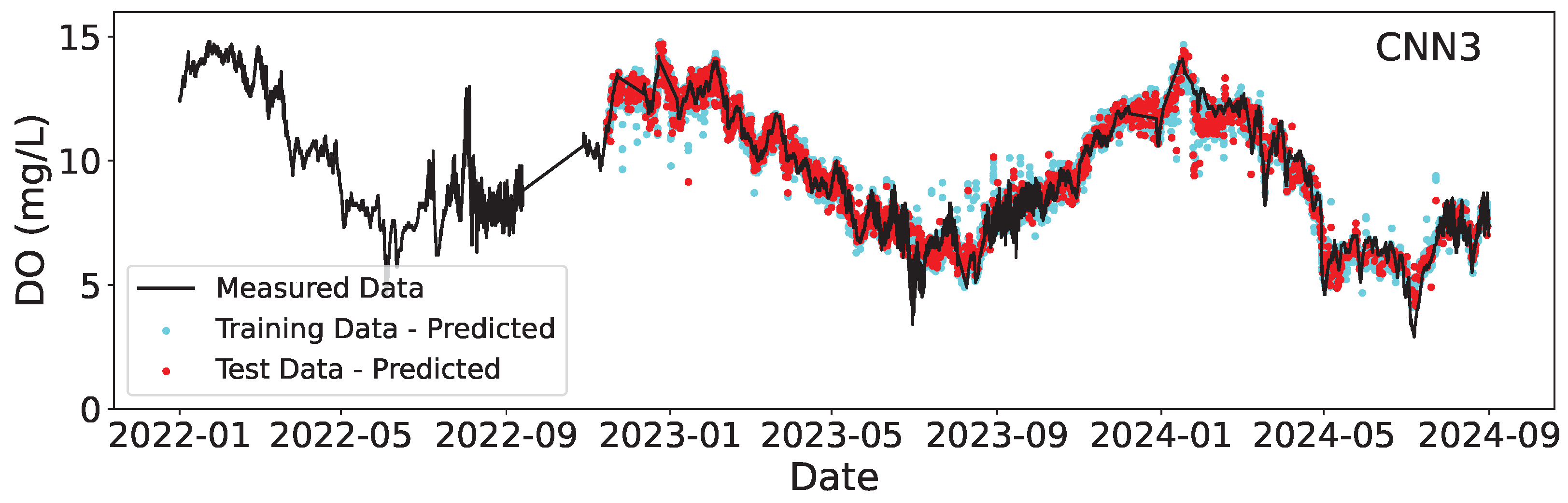
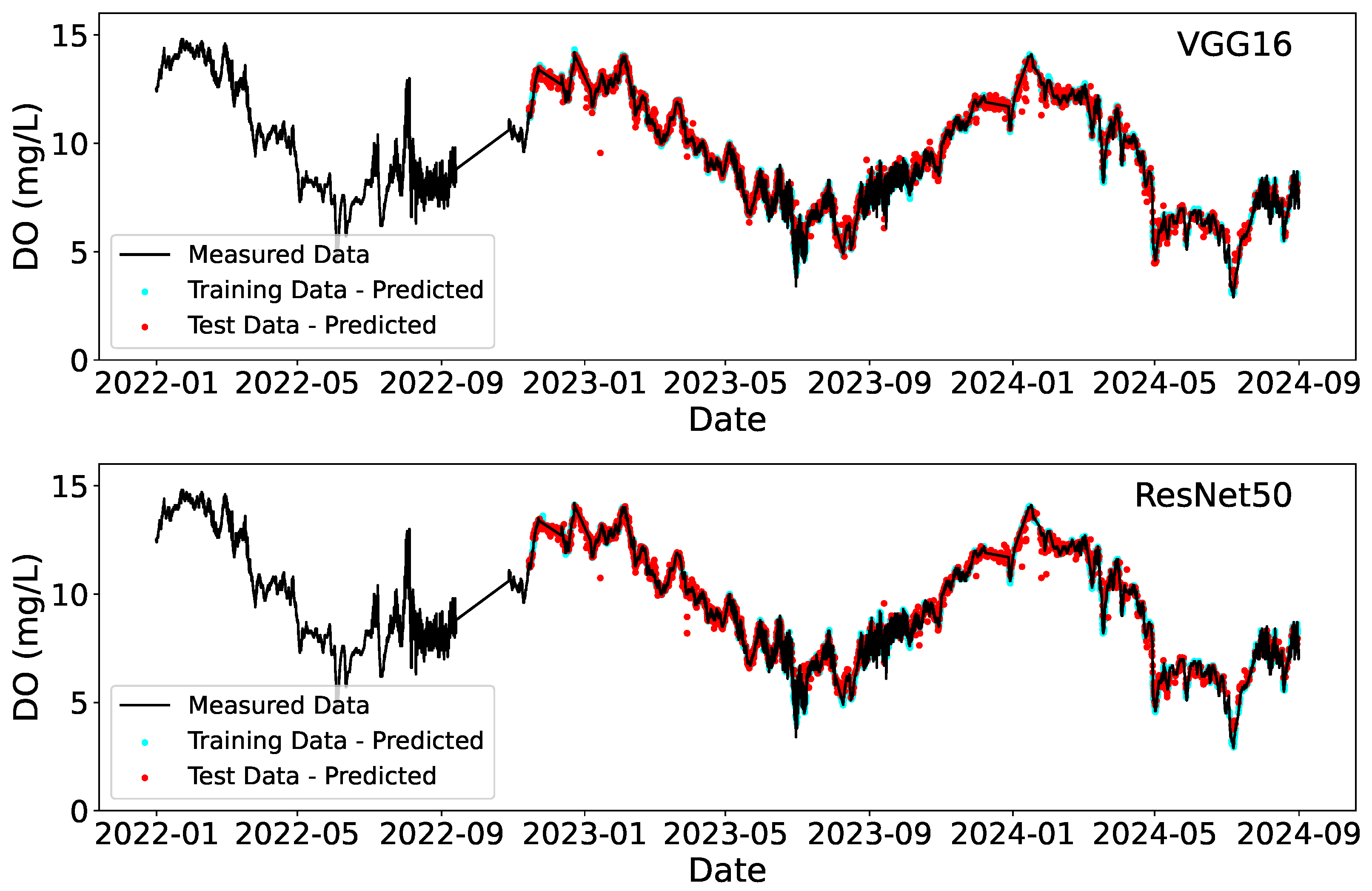
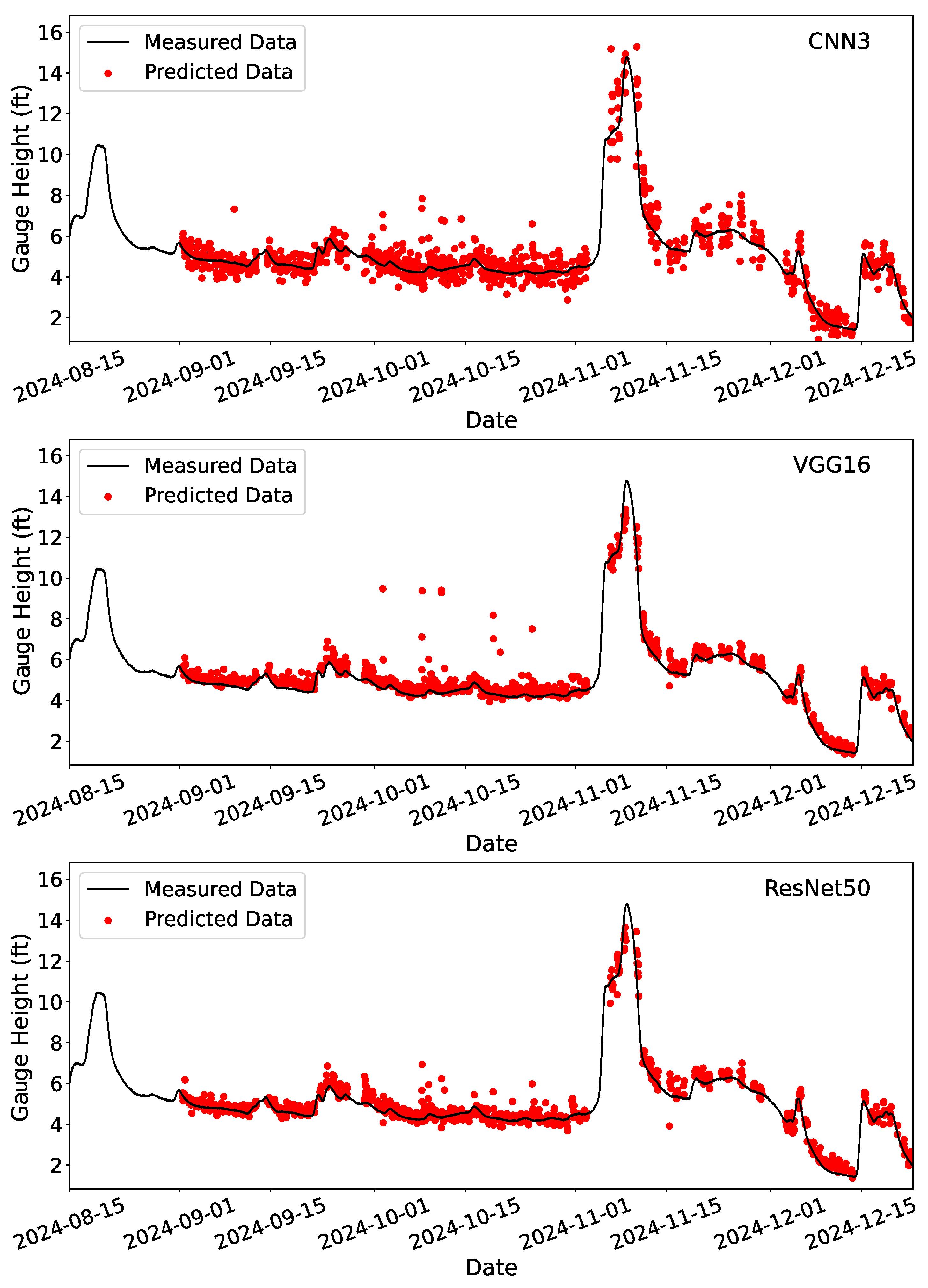
3.2. Deployment
4. Concluding Remarks
Author Contributions
Funding
Data Availability Statement
Conflicts of Interest
Abbreviations
| CNN | Convolutional neural network |
| DL | Deep learning |
| DO | Dissolved oxygen |
| fDOM | Fluorescent dissolved organic matter |
| FNU | Formazin nephelometric units |
| HIVIS | Hydrological Imagery Visualization and Information System |
| ML | Machine learning |
| QSE | Quinine sulfate equivalents |
| USGS | U.S. Geological Survey |
References
- Sutadian, A.; Muttil, N.; Yilmaz, A.; Perera, B.J.C. Development of river water quality indices—A review. Environ. Monit. Assess. 2016, 188, 58. [Google Scholar] [CrossRef]
- Nguyen, T.; Helm, B.; Hettiarachchi, H.; Caucci, S.; Krebs, P. The selection of design methods for river water quality monitoring networks: A review. Environ. Earth Sci. 2019, 78, 96. [Google Scholar] [CrossRef]
- Kuehne, L.; Dickens, C.; Tickner, D.; Messager, M.; Olden, J.; O’Brien, G.; Lehner, B.; Eriyagama, N. The future of global river health monitoring. PLoS Water 2023, 2, e0000101. [Google Scholar] [CrossRef]
- Falcone, J.A.; Carlisle, D.M.; Wolock, D.M.; Meador, M.R. GAGES: A stream gage database for evaluating natural and altered flow conditions in the conterminous United States. Ecology 2010, 91, 621. [Google Scholar] [CrossRef]
- Marti, M.; Heimann, D. Peak Streamflow Trends in Missouri and Their Relation to Changes in Climate, Water Years 1921–2020-F; U.S. Geological Survey Scientific Investigations Report 2023–5064, 50p; Chapter F of Peak Streamflow Trends and Their Relation to Changes in Climate in Illinois, Iowa, Michigan, Minnesota, Missouri, Montana, North Dakota, South Dakota, and Wisconsin; U.S. Geological Survey: Reston, VA, USA, 2024. [CrossRef]
- U.S. Geological Survey. A New Evaluation of the USGS Streamgaging Network; A Report to Congress; U.S. Geological Survey: Reston, VA, USA, 1998.
- Li, G.; Wang, B.; Elliott, C.M.; Call, B.C.; Chapman, D.C.; Jacobson, R.B. A three-dimensional Lagrangian particle tracking model for predicting transport of eggs of rheophilic-spawning carps in turbulent rivers. Ecol. Model. 2022, 470, 110035. [Google Scholar] [CrossRef]
- Li, G.; Elliott, C.M.; Call, B.C.; Chapman, D.C.; Jacobson, R.B.; Wang, B. Evaluations of Lagrangian egg drift models: From a laboratory flume to large channelized rivers. Ecol. Model. 2023, 475, 110200. [Google Scholar] [CrossRef]
- Xu, R.; Chapman, D.C.; Elliott, C.M.; Call, B.C.; Jacobson, R.B.; Wang, B. Ecological inferences on invasive carp survival using hydrodynamics and egg drift models. Sci. Rep. 2024, 14, 9556. [Google Scholar] [CrossRef]
- Tom, M.; Prabha, R.; Wu, T.; Baltsavias, E.; Leal-Taixé, L.; Schindler, K. Ice Monitoring in Swiss Lakes from Optical Satellites and Webcams Using Machine Learning. Remote Sens. 2020, 12, 3555. [Google Scholar] [CrossRef]
- Tedesco, M.; Radzikowski, J. Assessment of a Machine Learning Algorithm Using Web Images for Flood Detection and Water Level Estimates. GeoHazards 2023, 4, 437–452. [Google Scholar] [CrossRef]
- Bradley, E.S.; Toomey, M.P.; Still, C.J.; Roberts, D.A. Multi-scale sensor fusion with an online application: Integrating GOES, MODIS, and webcam imagery for environmental monitoring. IEEE J. Sel. Top. Appl. Earth Obs. Remote Sens. 2010, 3, 497–506. [Google Scholar] [CrossRef]
- Helmrich, A.M.; Ruddell, B.L.; Bessem, K.; Chester, M.V.; Chohan, N.; Doerry, E.; Eppinger, J.; Garcia, M.; Goodall, J.L.; Lowry, C.; et al. Opportunities for crowdsourcing in urban flood monitoring. Environ. Model. Softw. 2021, 143, 105124. [Google Scholar]
- Richardson, A.D.; Jenkins, J.P.; Braswell, B.H.; Hollinger, D.Y.; Ollinger, S.V.; Smith, M.L. Use of digital webcam images to track spring green-up in a deciduous broadleaf forest. Oecologia 2007, 152, 323–334. [Google Scholar]
- LeCun, Y.; Bengio, Y.; Hinton, G. Deep learning. Nature 2015, 521, 436–444. [Google Scholar]
- Tripathy, K.P.; Mishra, A.K. Deep learning in hydrology and water resources disciplines: Concepts, methods, applications, and research directions. J. Hydrol. 2024, 628, 130458. [Google Scholar]
- Pouyanfar, S.; Sadiq, S.; Yan, Y.; Tian, H.; Tao, Y.; Reyes, M.P.; Shyu, M.L.; Chen, S.C.; Iyengar, S.S. A survey on deep learning: Algorithms, techniques, and applications. ACM Comput. Surv. (CSUR) 2018, 51, 1–36. [Google Scholar]
- Sharifani, K.; Amini, M. Machine learning and deep learning: A review of methods and applications. World Inf. Technol. Eng. J. 2023, 10, 3897–3904. [Google Scholar]
- Janiesch, C.; Zschech, P.; Heinrich, K. Machine learning and deep learning. Electron. Mark. 2021, 31, 685–695. [Google Scholar]
- Maier, H.R.; Jain, A.; Dandy, G.C.; Sudheer, K. Methods used for the development of neural networks for the prediction of water resource variables in river systems: Current status and future directions. Environ. Model. Softw. 2010, 25, 891–909. [Google Scholar] [CrossRef]
- Kimura, N.; Yoshinaga, I.; Sekijima, K.; Azechi, I.; Baba, D. Convolutional Neural Network Coupled with a Transfer-Learning Approach for Time-Series Flood Predictions. Water 2020, 12, 96. [Google Scholar] [CrossRef]
- Kim, H.I.; Kim, D.; Mahdian, M.; Salamattalab, M.M.; Bateni, S.M.; Noori, R. Incorporation of water quality index models with machine learning-based techniques for real-time assessment of aquatic ecosystems. Environ. Pollut. 2024, 355, 124242. [Google Scholar] [CrossRef]
- Saravani, M.J.; Noori, R.; Jun, C.; Kim, D.; Bateni, S.M.; Kianmehr, P.; Woolway, R.I. Predicting Chlorophyll-a Concentrations in the World’s Largest Lakes Using Kolmogorov-Arnold Networks. Environ. Sci. Technol. 2025, 59, 1801–1810. [Google Scholar] [CrossRef]
- Eltner, A.; Bressan, P.O.; Akiyama, T.; Gonçalves, W.N.; Junior, J.M. Using Deep Learning for Automatic Water Stage Measurements. Water Resour. Res. 2021, 57, e2020WR027608. [Google Scholar] [CrossRef]
- Vandaele, R.; Dance, S.L.; Ojha, V. Deep learning for automated river-level monitoring through river-camera images: An approach based on water segmentation and transfer learning. Hydrol. Earth Syst. Sci. 2021, 25, 4435–4453. [Google Scholar] [CrossRef]
- Vanden Boomen, R.L.; Yu, Z.Y.; Liao, Q. Application of Deep Learning for Imaging-Based Stream Gaging. Water Resour. Res. 2021, 57, e2021WR029980. [Google Scholar] [CrossRef]
- Simonya, K.; Zisserman, A. Very deep convolutional networks for large-scale image recognition. In Proceedings of the International Conference on Learning Representations, San Diego, CA, USA, 7–9 May 2015. [Google Scholar]
- Ansari, S.; Rennie, C.D.; Jamieson, E.C.; Seidou, O.; Clark, S.P. RivQNet: Deep Learning Based River Discharge Estimation Using Close-Range Water Surface Imagery. Water Resour. Res. 2023, 59, e2021WR031841. [Google Scholar] [CrossRef]
- Dosovitskiy, A.; Fischer, P.; Ilg, E.; Häusser, P.; Hazırbaş, C.; Golkov, V.; Smagt, P.v.d.; Cremers, D.; Brox, T. FlowNet: Learning Optical Flow with Convolutional Networks. In Proceedings of the 2015 IEEE International Conference on Computer Vision, Santiago, Chile, 7–13 December 2015; pp. 2758–2766. [Google Scholar]
- Lopez-Fuentes, L.; Rossi, C.; Skinnemoen, H. River segmentation for flood monitoring. In Proceedings of the IEEE International Conference on Big Data (Big Data), Boston, MA, USA, 11–14 December 2017; pp. 3746–3749. [Google Scholar] [CrossRef]
- Moy de Vitry, M.; Kramer, S.; Wegner, J.D.; Leitão, J.P. Scalable flood level trend monitoring with surveillance cameras using a deep convolutional neural network. Hydrol. Earth Syst. Sci. 2019, 23, 4621–4634. [Google Scholar] [CrossRef]
- Pally, R.; Samadi, S. Application of image processing and convolutional neural networks for flood image classification and semantic segmentation. Environ. Model. Softw. 2022, 148, 105285. [Google Scholar] [CrossRef]
- Doerffer, R.; Schiller, H. The MERIS Case 2 water algorithm. Int. J. Remote Sens. 2007, 28, 517–535. [Google Scholar] [CrossRef]
- Gupta, A.; Ruebush, E. AquaSight: Automatic Water Impurity Detection Utilizing Convolutional Neural Networks. arXiv 2019, arXiv:1907.07573. [Google Scholar]
- Chen, J.; Zhang, D.; Yang, S.; Nanehkaran, Y.A. Intelligent monitoring method of water quality based on image processing and RVFL-GMDH model. IET Image Process. 2020, 14, 4646–4656. [Google Scholar] [CrossRef]
- Anand, V.; Oinam, B.; Wieprecht, S. Machine learning approach for water quality predictions based on multispectral satellite imageries. Ecol. Inform. 2024, 84, 102868. [Google Scholar] [CrossRef]
- He, K.M.; Zhang, X.Y.; Ren, S.Q.; Sun, J. Deep Residual Learning for Image Recognition. In Proceedings of the 2016 IEEE Conference on Computer Vision and Pattern Recognition (CVPR), Las Vegas, NV, USA, 27–30 June 2016; pp. 770–778. [Google Scholar] [CrossRef]
- Li, G.; Elliott, C.M.; Call, B.C.; Sansom, B.J.; Jacobson, R.B.; Wang, B. Turbulence near a sandbar island in the lower Missouri River. River Res. Appl. 2023, 39, 1857–1874. [Google Scholar] [CrossRef]
- Booth, A.; Fleck, J.; Pellerin, B.A.; Hansen, A.; Etheridge, A.; Foster, G.M.; Graham, J.L.; Bergamaschi, B.A.; Carpenter, K.D.; Downing, B.D.; et al. Field Techniques for Fluorescence Measurements Targeting Dissolved Organic Matter, Hydrocarbons, and Wastewater in Environmental Waters: Principles and Guidelines for Instrument Selection, Operation and Maintenance, Quality Assurance, and Data Reporting; U.S. Geological Survey Techniques and Methods, Book 1, Chap. D11, 41p; U.S. Geological Survey: Reston, VA, USA, 2023; 41p. [CrossRef]
- Dai, D. An introduction of cnn: Models and training on neural network models. In Proceedings of the 2021 International Conference on Big Data, Artificial Intelligence and Risk Management (ICBAR), Shanghai, China, 5–7 November 2021; pp. 135–138. [Google Scholar]
- Jing, Y.; Zhang, L.; Hao, W.; Huang, L. Numerical study of a CNN-based model for regional wave prediction. Ocean. Eng. 2022, 255, 111400. [Google Scholar] [CrossRef]
- Trang, N.T.H.; Long, K.Q.; An, P.L.; Dang, T.N. Development of an artificial intelligence-based breast cancer detection model by combining mammograms and medical health records. Diagnostics 2023, 13, 346. [Google Scholar] [CrossRef] [PubMed]
- Tammina, S. Transfer learning using vgg-16 with deep convolutional neural network for classifying images. Int. J. Sci. Res. Publ. (IJSRP) 2019, 9, 143–150. [Google Scholar] [CrossRef]
- Khan, M.A.; Ahmed, N.; Padela, J.; Raza, M.S.; Gangopadhyay, A.; Wang, J.; Foulds, J.; Busart, C.; Erbacher, R.F. Flood-ResNet50: Optimized Deep Learning Model for Efficient Flood Detection on Edge Device. In Proceedings of the 2023 International Conference on Machine Learning and Applications (ICMLA), Jacksonville, FL, USA, 15–17 December 2023; pp. 512–519. [Google Scholar]
- Prakash, S.; Sharma, A.; Sahu, S.S. Soil moisture prediction using machine learning. In Proceedings of the 2018 Second International Conference on Inventive Communication and Computational Technologies (ICICCT), Coimbatore, India, 20–21 April 2018; pp. 1–6. [Google Scholar]
- Luan, H.; Tsai, C.C. A review of using machine learning approaches for precision education. Educ. Technol. Soc. 2021, 24, 250–266. [Google Scholar]
- Lange, H.; Sippel, S. Machine learning applications in hydrology. In Forest-Water Interactions; Springer: Cham, Switzerland, 2020; pp. 233–257. [Google Scholar]


| CNN3 | VGG16 | ResNet50 | |||
|---|---|---|---|---|---|
| Gauge height (ft) | R2 | Training | 0.981 | 0.998 | 0.998 |
| R2 | Testing | 0.959 | 0.986 | 0.982 | |
| RMSE | Training | 0.58 | 0.18 | 0.20 | |
| RMSE | Testing | 0.86 | 0.50 | 0.57 | |
| Turbidity (FNU) | R2 | Training | 0.791 | 0.986 | 0.986 |
| R2 | Testing | 0.627 | 0.728 | 0.743 | |
| RMSE | Training | 41.06 | 10.65 | 10.47 | |
| RMSE | Testing | 56.57 | 48.31 | 48.99 | |
| fDOM (μg/L in QSE) | R2 | Training | 0.890 | 0.997 | 1.000 |
| R2 | Testing | 0.675 | 0.886 | 0.890 | |
| RMSE | Training | 0.68 | 0.12 | 0.02 | |
| RMSE | Testing | 1.14 | 0.68 | 0.66 | |
| DO (mg/L) | R2 | Training | 0.954 | 0.999 | 1.000 |
| R2 | Testing | 0.944 | 0.986 | 0.987 | |
| RMSE | Training | 0.51 | 0.07 | 0.03 | |
| RMSE | Testing | 0.57 | 0.28 | 0.28 |
| CNN3 | VGG16 | ResNet50 | ||
|---|---|---|---|---|
| Gauge height (ft) | R2 | 0.843 | 0.892 | 0.945 |
| RMSE | 0.67 | 0.56 | 0.40 | |
| Turbidity (FNU) | R2 | −0.371 | −0.077 | 0.315 |
| RMSE | 34.09 | 30.22 | 24.11 | |
| fDOM (μg/L in QSE) | R2 | −0.050 | −0.015 | 0.227 |
| RMSE | 1.52 | 1.49 | 1.30 | |
| DO (mg/L) | R2 | 0.752 | 0.759 | 0.703 |
| RMSE | 0.72 | 0.71 | 0.79 |
Disclaimer/Publisher’s Note: The statements, opinions and data contained in all publications are solely those of the individual author(s) and contributor(s) and not of MDPI and/or the editor(s). MDPI and/or the editor(s) disclaim responsibility for any injury to people or property resulting from any ideas, methods, instructions or products referred to in the content. |
© 2025 by the authors. Licensee MDPI, Basel, Switzerland. This article is an open access article distributed under the terms and conditions of the Creative Commons Attribution (CC BY) license (https://creativecommons.org/licenses/by/4.0/).
Share and Cite
Xu, R.; Wang, B. Assessing Deep Learning Techniques for Remote Gauging and Water Quality Monitoring Using Webcam Images. Hydrology 2025, 12, 65. https://doi.org/10.3390/hydrology12040065
Xu R, Wang B. Assessing Deep Learning Techniques for Remote Gauging and Water Quality Monitoring Using Webcam Images. Hydrology. 2025; 12(4):65. https://doi.org/10.3390/hydrology12040065
Chicago/Turabian StyleXu, Ruichen, and Binbin Wang. 2025. "Assessing Deep Learning Techniques for Remote Gauging and Water Quality Monitoring Using Webcam Images" Hydrology 12, no. 4: 65. https://doi.org/10.3390/hydrology12040065
APA StyleXu, R., & Wang, B. (2025). Assessing Deep Learning Techniques for Remote Gauging and Water Quality Monitoring Using Webcam Images. Hydrology, 12(4), 65. https://doi.org/10.3390/hydrology12040065