Article

Dependence of Soil Moisture and Strength on Topography and Vegetation Varies Within a SMAP Grid Cell

by
Joseph R. Bindner
1,
Holly Proulx
1,
Kevin Wickham
1,
Jeffrey D. Niemann
1,*,
Joseph Scalia IV
1,
Timothy R. Green
2 and
Peter J. Grazaitis
3
1
Department of Civil and Environmental Engineering, Campus Delivery 1372, Colorado State University, Fort Collins, CO 80523, USA
2
Water Management & Systems Research Unit, Agricultural Research Service, USDA, 2150-D Center Ave., Fort Collins, CO 80526, USA
3
U.S. Army DEVCOM Analysis Center, Complex Ground Systems Branch (FCDD-DAS-LHC), 7101 Mulberry Point Road, BLDG 459, Aberdeen Proving Ground, Aberdeen, MD 21005, USA
*
Author to whom correspondence should be addressed.
Hydrology 2025, 12(2), 34; https://doi.org/10.3390/hydrology12020034
Submission received: 9 January 2025 / Revised: 6 February 2025 / Accepted: 11 February 2025 / Published: 15 February 2025
(This article belongs to the Section Soil and Hydrology)

Abstract

:
Off-road vehicle mobility assessments rely on fine-resolution (~10 m) estimates of soil moisture and strength across the region of interest. Such estimates are often produced by downscaling soil moisture from a microwave satellite like SMAP, then using the soil moisture in a soil strength model. Soil moisture downscaling methods typically assume consistent relationships between the moisture and topographic, vegetation, and soil composition characteristics within the microwave satellite grid cells. The objective of this study is to examine whether soil moisture and strength exhibit heterogenous dependencies on topography, vegetation, and soil composition characteristics within a SMAP grid cell. Soil moisture and strength data were collected at four geographically separated regions within a 9 km SMAP grid cell in the Front Range foothills of northern Colorado. Laboratory methods and pedotransfer functions were used to characterize soil attributes, and remote sensing data were used to determine topographic and vegetation attributes. Pearson correlation analyses were used to quantify the direction, strength, and significance of the relationships of both soil moisture and strength with topography, vegetation, and soil composition. Contrary to the common assumption, spatial variations in the slope and correlation of the relationships are observed for both soil moisture and strength. The findings indicate that improved predictions of soil moisture and soil strength may be achievable by soil moisture downscaling procedures that use spatially variable parameters across the downscaling extent.

1. Introduction

Understanding surficial soil strength across a landscape is important for assessing vehicle mobility for agricultural, recreational, land management, and other purposes [1,2,3,4]. Soil strength can be highly variable due to fine-resolution (5 to 30 m) variations in soil moisture and soil texture (percentage of gravel, sand, silt, and clay) [5]. Therefore, fine-resolution soil strength estimates are required to capture spatial variations and adequately characterize vehicle mobility.
For vehicle mobility applications, surficial soil strength is commonly quantified using the rating cone index (RCI), which is calculated by multiplying the cone index (CI) by the remold index (RI) (The Abbreviations section provides a complete list of acronyms) [6]. The cone index can be measured in the field by pressing a cone penetrometer into the soil profile at a constant rate and measuring the pressure required to advance the cone. The remold index quantifies the tendency of a soil to lose strength under vehicle loading and is determined on a remolded soil sample [6]. For coarse grained soils, the RI is one, so RCI and CI are interchangeable.
Field measurement of RCI is impractical across large spatial extents, so the RCI is often inferred from soil composition and moisture information. For example, the Strength of Surface Soils (STRESS) model uses average soil strength and soil–water retention characteristics from texture classifications to estimate fine-resolution surficial soil strength [7]. Other soil strength modeling procedures include the North Atlantic Treaty Organization Reference Mobility Model (NRMM), which empirically estimates vehicle mobility based on vehicle, terrain, and environmental factors [8,9,10]. McCollough et al. [11] introduced the Next Generation NRMM (NG-NRMM), which implements complex terramechanics models [12] and requires a comprehensive understanding of soil properties. However, obtaining high-fidelity, fine-resolution soil moisture and soil composition data can be difficult.
Soil moisture products are available nearly globally from microwave satellites with grid cells ranging from 9 to 60 km. Such products are generated by the Tropical Rainfall Measuring Mission (TRMM) [13], Advanced Scatterometer (ASCAT) [14], Advanced Microwave Scanning Radiometer 2 (AMSR2) [15], Soil Moisture Ocean Salinity (SMOS) [16], and Soil Moisture Active Passive (SMAP) [17] satellites. However, these datasets do not have the fine spatial resolution needed for soil strength and vehicle mobility modeling. Various methods have been proposed to downscale coarse-resolution soil moisture data. Coarse-resolution microwave data have been downscaled to 1 km grid cells based on fine-resolution soil temperature and land–atmosphere interaction parameters [18]. Optical/thermal data are available at fine resolutions (tens of meters) and can be used to directly estimate fine-resolution soil moisture based on vegetation indices from optical data and land-surface temperatures from thermal data [19]. Data from optical/thermal sources have also been used for soil moisture downscaling procedures [20,21]. Other approaches for downscaling soil moisture rely on relationships between soil moisture and topographic, vegetation, and soil attributes. Some of these methods have used machine learning approaches [22,23], while others have used mechanistic models [24]. For example, the Equilibrium Moisture from Topography, Vegetation, and Soil (EMT+VS) model [25,26,27,28] can be used to downscale soil moisture to 10 to 30 m grid cells using fine-resolution topographic, vegetation, and soil data.
Soil moisture downscaling methods that are informed by soil and landscape attributes typically assume that the relationships between soil moisture and topography, vegetation, and soil composition are constant throughout a coarse-resolution grid cell [27]. Ali et al. [29] studied the spatial relationships between soil moisture and topographic variables at different scales in a humid, forested environment and found that for larger extents (0.54 ha–1.4 ha), the dependence of soil moisture on topography is significant, but for smaller extents (0.02 ha–0.54 ha), topography does not have strong correlations to soil moisture. Furthermore, soil moisture estimates can be inaccurate when model parameters are adjusted uniformly for the entire modeling extent [30], which indicates non-uniform relationships between soil moisture and soil and landscape attributes. Yu et al. [31] conducted statistical analyses on the effects of micro-topography and vegetation type on soil moisture in a large semiarid gully (49 ha) and found that soil moisture has varying dependence on topographic attributes, depending on the location within the catchment. Additionally, Liang et al. [32] studied the dependence of soil moisture on topographic, soil, and vegetation features at a site (0.16 ha) within a small headwater catchment and determined that soil moisture is most strongly correlated with different topographic, soil, and vegetation features within various portions of the catchment. While such studies have highlighted the variability in soil moisture dependencies within small spatial extents [33,34,35,36,37], there is less understanding of how soil moisture dependence varies within the spatial extent of a microwave remote sensing grid cell. Fatholoumi et al. [38] examined soil moisture heterogeneity using soil moisture observations at 148 locations within a 567 km2 watershed with complex mountainous topography and diverse landcover types. They found that soil moisture’s correlation with regional characteristics varied as the data were binned in different ways (e.g., based on aspect or slope). No study has examined the possible dependence of soil strength (viz. RCI) on topographic, soil, and vegetation characteristics across a large region. An improved understanding of how these dependencies vary within such extents may better inform soil moisture and associated soil strength modeling procedures.
The objective of this study is to examine the spatial variability in the dependence of both soil moisture and soil strength on topographic, vegetation, and soil composition attributes across a 9 km SMAP grid cell. SMAP was used to define the spatial extent because it has a higher spatial resolution than other passive microwave products, and its accuracy has been demonstrated for this region [39]. Four geographically separated regions with varying soil, topography, and vegetation were selected within a 9 km region. Soil moisture and soil strength were measured at 86 sampling locations on 10 dates between May and August of 2022. Soil samples were collected at each sampling location and used to determine soil texture, plasticity, and organic content. Landscape attributes were derived from a digital elevation model (DEM), and vegetation indices were determined from multispectral satellite products. The Pearson correlation coefficient (r) was used to quantify the dependence of soil moisture and soil strength on soil and landscape attributes within each sampling region, and Pearson p-values were used to assess the statistical significance of the correlations. To assess how the significant relationships deviate from the average behavior, the relationship slopes in each region were compared to the slopes for the entire dataset.

2. Materials and Methods

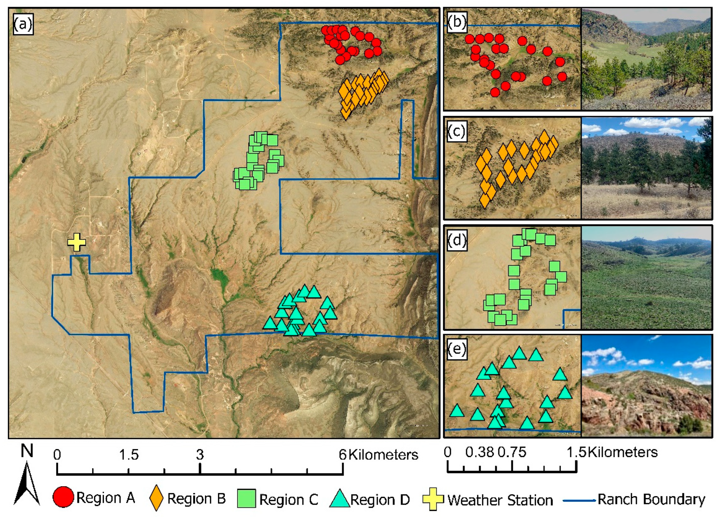
2.1. Study Site and Sampling Strategy

The study site (Maxwell Ranch) is approximately 50 km northwest of Fort Collins, Colorado, in the Laramie Foothills (located between the Great Plains and the Rocky Mountains). Maxwell Ranch includes 4000 ha of land and spans much of a single 9 km grid cell of the SMAP Enhanced Level 3 Radiometer product (Figure 1a) [40,41]. Elevations at the site range from 1964 m to 2286 m, with an average slope of 0.22 m/m. Soils are predominately coarse loams weathered from granite and (to a lesser extent) sandstone. Vegetation includes grasses, shrubs (primarily Antelope Bitterbrush and Mountain Mahogany), and pine forests (primarily Ponderosa and Piñon pine) [39].
Four sampling regions (A, B, C, and D) were selected to observe the varying topography, vegetation, and soil conditions at the study site (Figure 1a). Region A is in the northernmost portion of the study site and has forested hillslopes and a grassy valley bottom with a stream (Figure 1b). Region B consists of hills with open-canopy Ponderosa pine forests (Figure 1c). Region C is comprised of grassy hills around a grassy valley bottom containing a stream (Figure 1d). Region D is located near the southern boundary of the study site. It is predominately vegetated by Mountain Mahagony shrubs and has several rock outcrops (Figure 1e). Within each region, sampling locations were selected to observe the range of soil, topography, and vegetation conditions in the region. The topographic, vegetation, and soil characteristics considered have been shown to be important to soil moisture variability and downscaling in prior studies (see further discussion below) [26,27,42,43,44,45]. The range for each characteristic was divided into bins of equal probability of occurrence within the SMAP grid cell. Sampling locations within the bins were selected based on practical considerations such as accessibility. Regions A, B, C, and D contain 22, 22, 24, and 18 sampling locations, respectively.
The site is in a semi-arid continental climate and receives approximately 430 mm of annual precipitation, with most precipitation occurring during the winter as snowfall. Soil moisture and strength sampling were conducted between May and August of 2022 to avoid the frozen soil and snow cover that can occur during winter. A private weather station (KCOLIVER 12) is located immediately west of the ranch. Figure 2 shows the daily precipitation during the study period. The largest precipitation events occurred on 31 May and 28 July. Field dates were selected to span a wide range of moisture conditions. Thus, sampling was primarily performed immediately after these precipitation events and on subsequent dates as the soil dried (Figure 2).

2.2. Data Collection

2.2.1. Topography and Vegetation

Remote sensing products were used to characterize topography and vegetation at the sampling locations and across the 9 km SMAP grid cell. The 10 m DEM was obtained from the National Elevation Dataset [46] and processed via Terrain Analysis Using DEM tools in ArcGIS Pro version 3 (TauDEM) [47]. Topographic attributes considered include elevation, log of specific contributing area (log SCA), slope, cosine of aspect, and potential solar radiation index (PSRI) for the summer solstice, which is calculated using slope, aspect, latitude, and date of the summer solstice [48,49,50].
The density of green vegetation cover was characterized using 10 m multispectral imagery from the Sentinel 2 satellite [51]. Due to cloud cover on multiple dates during the study period, a single image from 26 May was used to calculate the normalized difference vegetation index (NDVI) [52] and enhanced vegetation index (EVI) [53,54]. NDVI uses only the red and near-infrared bands, while EVI also uses the blue band.
The Soil Survey Geographic (SSURGO) database was used to obtain percentage of sand, silt, and clay using the U.S. Department of Agriculture (USDA) definitions [55].

2.2.2. Soil Moisture

Surface soil moisture (θ; cm3/cm3) was measured at each sampling location and date using a Stevens HydraProbe Soil Sensor [56]. On some dates, thunderstorms prevented data collection at some locations. The HydraProbe has four 5.7 cm long, 0.3 cm diameter measurement tines and uses dielectric impedance to determine soil moisture with an accuracy of ±0.03 cm3/cm3 and precision of ±0.001 cm3/cm3 [56]. At each sampling location, leaf litter was temporarily removed, and three HydraProbe measurements were collected (with the probe inserted vertically) within approximately 1 m of the sampling location and averaged to determine the soil moisture of the sampling location.

2.2.3. Soil Strength

Soil strength was measured using a cone penetrometer with a 6.45 cm2 cone and load cell with 0.7 kPa accuracy [57]. The penetrometer cone tip was advanced into the soil at a constant rate until the cone base reached 2.5 cm below the soil surface. The cone penetrometer measures the force required to advance the cone into the soil, which can be divided by the cone area to produce CI. The RI was not measured for fine-grained soils at the site (which are rare), so the CI (kPa) is used to characterize soil strength. Three cone penetrometer measurements were collected within approximately 1 m of each sampling location and averaged to determine the soil strength for that sampling location.

2.2.4. Soil Composition

Soil samples were collected at each sampling location for laboratory analysis. Three soil samples were collected within approximately 1 m of each sampling location and within approximately the top 5 cm of the soil surface. Vegetation and leaf litter were removed from the soil surface prior to sampling. The three soil samples were collected at each sampling location and combined for laboratory analyses.
Sedimentation analysis was completed using the PARIO Soil Particle Analyzer to characterize the distribution of particles ranging in size from 2 to 63 µm according to the PARIO classic procedure (mass fraction detection error is ±0.03 g/g) [58]. Representative sedimentation specimens were obtained according to the moist specimen procurement procedure in ASTM D7928 [59]. PARIO data evaluation was based on the integral suspension pressure method [60]. The distribution of soil particle sizes greater than 75 µm was characterized using mechanical sieve analysis, which was performed following ASTM D6913 [61]. Representative sieve specimens were obtained according to the moist specimen procurement procedure, and the 25.4 mm, 19.0 mm, 9.5 mm, No. 4, No. 10, No. 20, No. 40, No. 60, No. 100, and No. 200 sieves were used.
The laboratory results were used to determine percentage of sand, silt, and clay (after removal of gravel) based on the USDA particle size ranges. Porosity and saturated hydraulic conductivity Ks were estimated using percentage of sand and clay in pedotransfer functions [62]. Percentage of sand, silt, and clay were also used to determine the USDA soil classification [63]. Particle-size distributions were used to determine the particle diameter corresponding to 10% mass finer (D10), 30% mass finer (D30), 60% mass finer (D60), and coefficient of uniformity (Cu). The parameter Cu is the ratio of D60 to D10 and provides information about the soil gradation (i.e., sorting) where greater values correspond to more well-graded (poorly sorted) soils.
Soil plasticity testing is used to inform soil classification in the Unified Soil Classification System (USCS) for soils with more than 5% fines. Soil plasticity testing was conducted to obtain soil liquid limit (LL), plastic limit (PL), and plasticity index (PI) following ASTM D4318 [64]. Samples were prepared using the dry preparation procedure. The LL was determined using the multipoint method, which typically has greater precision than the one-point method [64]. The PL was determined using the hand rolling procedure [64]. The USCS classification was determined following ASTM D2487 [65] and based on the particle size distribution, as well as the LL and PI.
Soil organic content was also determined. Organic content was calculated using ASTM D2974 Method A [66] to the nearest percentage of total dry mass.

2.3. Correlation and Slope Analyses

Pearson correlation analyses were used to examine the strength of linear relationships between different variables in the dataset, including relationships between topographic, vegetation, and soil attributes. Variations in the correlations between the different sub-regions are used to examine whether the strengths of the relationships vary within the SMAP grid cell. Relationships are considered statistically significant if the Pearson p-value is less than 0.05. Pearson correlations are used because prior studies have demonstrated linear correlations between many of these variables [26,27,42,43,44]. The analyses were also repeated using Spearman rank correlations and similar qualitative results occurred. We then utilize the slope of each relationship to characterize the form of the relationship. Variations in the slopes between sub-regions would indicate that the forms of the relationships vary within the SMAP grid cell.

3. Results

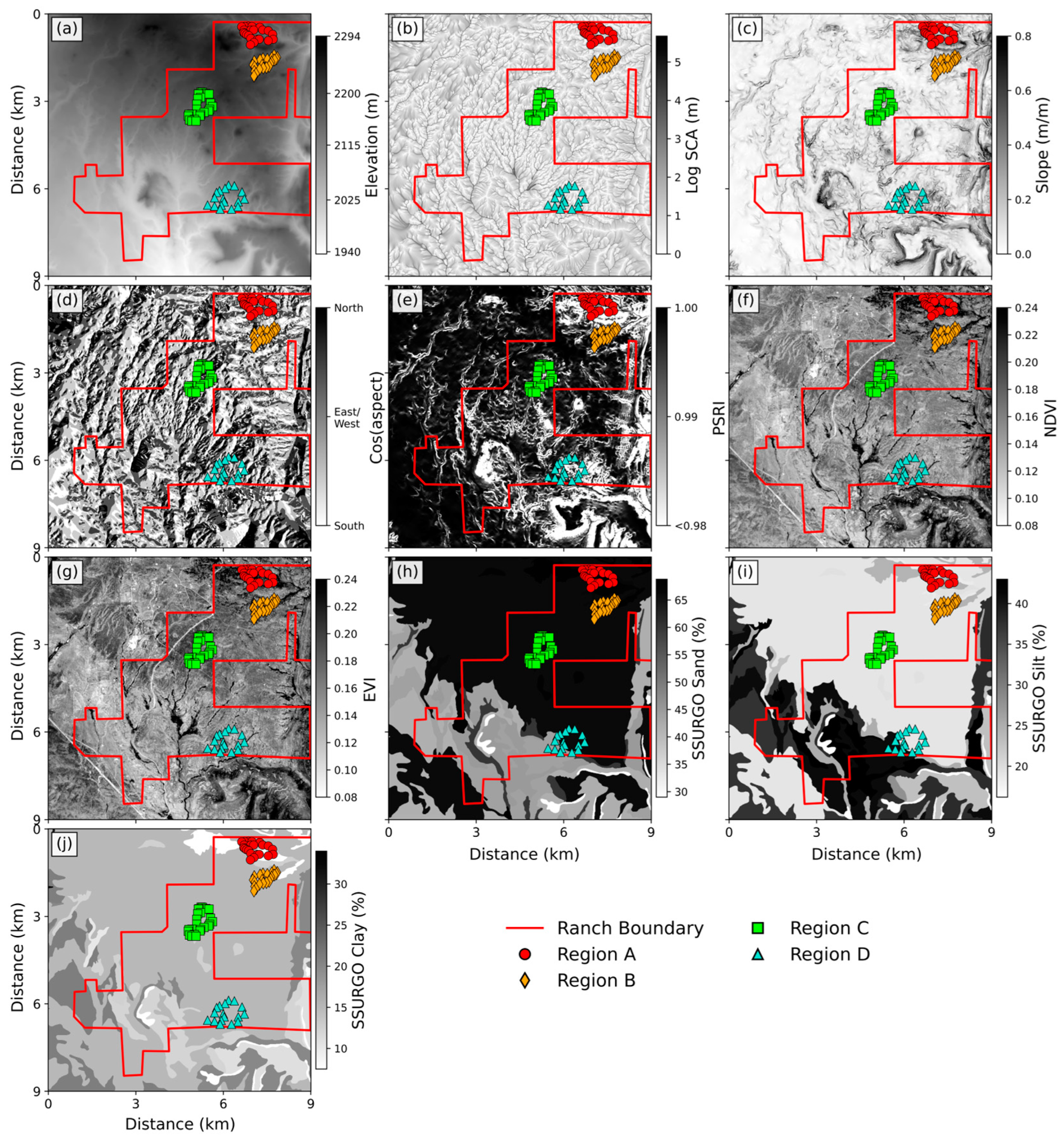
3.1. Topography, Vegetation, and SSURGO

Figure 3 shows maps of the topographic attributes, vegetation indices, and the USDA percentage of sand, silt, and clay from SSURGO. Elevation generally increases from south to north on the ranch (Figure 3a). The sampling points in Region D have the lowest average elevation (2067 m), while the points in Regions A, B, and C have similar average elevations (2163, 2172, and 2171 m, respectively). The topography is more variable at the north and south ends of the ranch (Figure 3c). The sampling points in Regions A and D have steeper slopes (averages of 0.28 and 0.20 m/m, respectively) than points in Regions B and C (averages of 0.17 and 0.16 m/m, respectively). Vegetation cover is greater on the north side of the ranch due to greater forest cover (Figure 3f,g). The NDVI is greater for the points in Regions A and B (averages of 0.22 and 0.22, respectively) than the points in Regions C and D (averages of 0.20 and 0.18, respectively). The EVI values follow similar patterns to the NDVI values. According to SSURGO, the soil is relatively uniform across the ranch, and only a few distinct soil types occur (Figure 3h–j). SSURGO suggests that Regions B and C have typical soil texture for the ranch. SSURGO also suggests that Region A has more silt and less clay than Regions B and C, and Region D has less sand and more silt than Regions B and C.
Figure 4 compares the histograms of the topographic, vegetation, and SSURGO soil composition attributes for the sampling locations and the entire SMAP grid cell. For most attributes, the histogram for the sampling locations resembles the histogram for the SMAP grid cell. However, the sampling locations have more points at high elevations (Figure 4a) and steeper slopes (Figure 4c) than the larger SMAP grid cell. Nonetheless, the similarity of the histograms for the topographic, vegetation, and soil characteristics suggests that the collection of sampling locations is representative of the larger SMAP region.

3.2. Laboratory Soil Composition

Figure 5a displays the USDA texture classifications of the soils collected at the sampling locations. Most soils are classified as sand, loamy sand, sandy loam, sandy clay loam, and loam. Contrary to SSURGO, the soils from Region D have the highest average USDA percentage of sand (75%), which is approximately 10% higher than Regions A, B, and C (averages of 66%, 66%, and 65%, respectively). Regions B and C do not contain any soil classified as USDA sand. The soils from Regions A, B, C, and D have a similar average USDA percentage of silt (20%, 20%, 23%, and 19%, respectively). The soils from Regions A and B have a higher average clay content (13% and 14%, respectively) than Regions C and D (8% and 5%, respectively). The higher clay content in Region A again conflicts with SSURGO.
As displayed in the soil plasticity chart (Figure 5b), the soils generally have a LL below 50 and plot below the A-line, which distinguishes silts and clays. The predominant fines classifications are low-plasticity silt and low-plasticity organic (ML or OL). Soils in Regions A and C have the highest average soil plasticity (LL ≈ 50%; PL ≈ 42%) compared to LL ≈ 44% and PL ≈ 39% in Regions B and D. Using the USCS soil classification system, 67% of the soils at sampling locations are classified as silty sand (SM), and 16% are classified as gravels. A few sampling locations are classified as high plasticity silt (MH), poorly graded sand (SP), and silty clayey sand (SC-SM). Several samples were classified as peat according to the ASTM D2487 standard [65]. Soil organic content ranges from 1% to 70% at the sampling locations. Regions B and C contain greater average soil organic content (14% and 15%, respectively) compared to Regions A and D (9% and 8%, respectively).

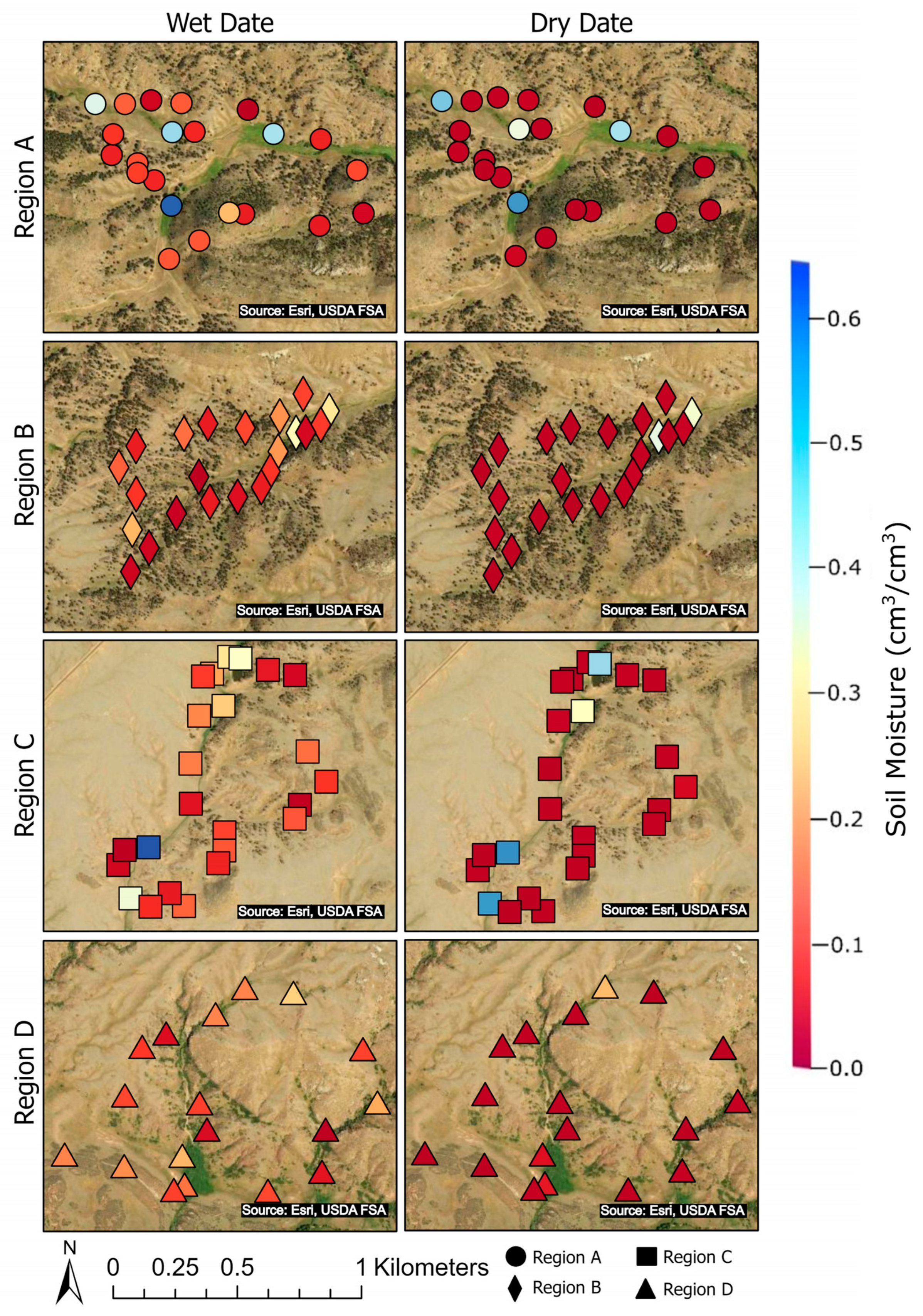
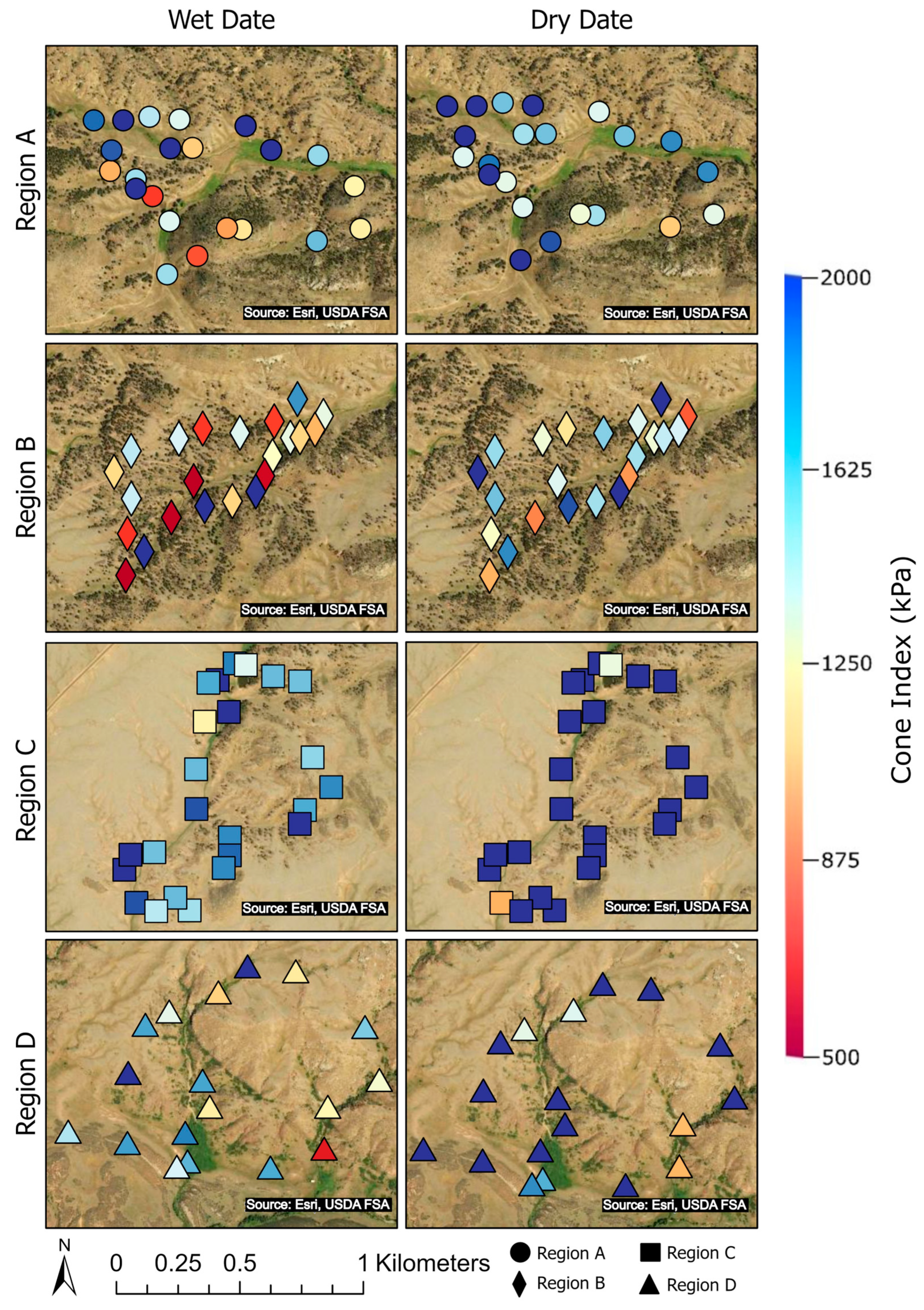
3.3. Soil Moisture and Strength

Figure 2 compares the average soil moisture ( θ ¯ ) from the field measurements and SMAP on each sampling date. The difference between the average soil moisture from the field measurements and SMAP was usually less than 0.05 cm3/cm3. The greatest difference is observed on 5 July because a precipitation event occurred within the SMAP grid cell but not in the sampling regions (based on visual observations and precipitation data in Figure 2). Nonetheless, these results suggest that the collection of field measurements is consistent with the SMAP grid cell as a whole.
Figure 6 shows the soil moisture observations from a representative wet date and dry date. The wet locations tend to occur in the valley bottoms, and their moisture remains consistent between dates. The drier locations on the hillslopes vary more between the dates. Figure 7 shows the histogram of soil moisture for each sampling region and date. Most soil moisture measurements are less than 0.25 cm3/cm3, with only a few measurements exceeding that value. Regions A and C have more sampling locations with soil moisture greater than 0.25 cm3/cm3 than the other regions. These locations often occur near the streams in Regions A and C, and they produce greater average soil moisture for Regions A and C (Regions B and D do not have streams). Region D contains very few wet observations. Sampling locations with the highest soil moisture are generally classified as USCS peat, which can have high porosity [67]. Maps of soil moisture for all sampling dates can be found in the Supplemental Material (Figure S1).
Soil strength (CI) maps for a representative wet and dry date are shown in Figure 8. CI is highly variable among sampling locations and among dates at a given sampling location. Figure 9 shows the histograms of CI for each region and sampling date. Regions A and B typically have similar distributions of soil strength, while Regions C and D are more dissimilar. On every date, the distribution of at least one region differs notably from the distributions in the other regions. On 2 August, for example, Region D’s cone index is approximately uniformly distributed between about 800 kPa and 2000 kPa, while the other regions have a clear peak in their distributions between 1500 kPa and 2000 kPa. Maps of soil strength for all sampling dates can be found in the Supplemental Material (Figure S2).

3.4. Relationships Between Soil Moisture/Strength and Regional Attributes

Figure 10a displays the Pearson correlations between the vegetation indices (NDVI and EVI) and the topographic attributes for each region. In Region A, the vegetation indices are significantly correlated with log(SCA), slope, and cos(aspect). The correlations indicate that thicker vegetation occurs in valley bottoms, flatter slopes, and north-facing aspects. In Region C, the vegetation indices are again significantly correlated with slope but also with PSRI (thicker vegetation occurs at locations receiving more summer sun). The vegetation indices in Regions B and D generally have weak correlations with the topographic attributes. Overall, these results suggest that the vegetation patterns differ between all four sampling regions.
Figure 10b displays the correlations between the soil composition attributes and the topographic and vegetation attributes for each sampling region. Overall, the soil attributes are better predicted by the vegetation indices than the topographic indices. The correlations between the soil attributes and vegetation indices are stronger in Regions A and C and weaker in Regions B and D. The soil attributes have similar correlations to EVI and NDVI. The correlations between the soil attributes and the topographic attributes vary among regions. Overall, they are strongest in Region A and weakest in Region C. In Region A, log SCA and cos(aspect) are the best predictors (among the topographic attributes) of soil composition. The correlations imply that finer soils tend to occur in valley bottoms and on north-facing slopes. In Regions B and D, the soil attributes are best predicted by slope and PSRI, with finer soils occurring on flatter slopes and slopes that receive more summer insolation.
Figure 11a displays the Pearson correlations between the soil moisture on different dates and the topographic, vegetation, and soil composition attributes. Overall, soil moisture is predicted better by vegetation and soil composition than topography. However, the correlations between soil moisture and the vegetation indices vary among regions. They are stronger for Regions A and C and weaker for Regions B and D (similar to the previously noted correlations between soil composition and vegetation). Soil moisture has similar correlations to NDVI and EVI, which again mimics the soil composition results and suggests that wetter conditions occur where vegetation is thicker.
The correlations between soil moisture and topography also vary between the sampling regions (Figure 11a). These correlations are strongest in Region A, moderate in Region B, and weak in Regions C and D. The most important topographic attributes for predicting soil moisture vary among regions. In Region A, soil moisture is most correlated with log SCA, slope, and cos(aspect) (again, similar to the earlier soil composition results). These correlations suggest that wetter conditions occur in valley bottoms, on flatter slopes, and on north-facing aspects. In Region B, soil moisture is most correlated with log SCA and elevation.
The correlations between soil moisture and soil composition also vary substantially between the regions (Figure 11a). They are generally stronger in Regions A and C and weaker in Regions B and D. The most important composition variables for predicting soil moisture vary among the regions. Soil moisture is strongly correlated with the USDA percentage of sand and USCS fines in all regions except Region D, suggesting that wetter conditions occur in soils with a high percentage of fines (silt and clay). Soil moisture is strongly correlated with the USDA percentage of clay only in Regions A and C, indicating that clayey soils (which correspond with denser green vegetation in Regions A and C, as noted earlier) are generally wetter. Soil moisture is strongly correlated with LL, PL, and organic content for all regions except Region B which, again, supports the interdependence between soil moisture, vegetation, and soil composition characteristics.
Figure 11b also shows the correlations between soil strength (viz. CI) and the topographic, vegetation, and soil attributes. Overall, soil strength has weak correlations with the explanatory variables, and the correlations are weaker for the topographic and vegetation attributes than the soil composition characteristics. In Region A, CI has significant negative correlations with elevation on several dates, but significant correlations with elevation are not observed in other regions. In Regions B and D, CI is negatively correlated with slope and positively correlated with PSRI on several dates, but CI has weak and inconsistent correlations with these variables in the other regions. In Region C, CI has the most frequent significant correlations with cos(aspect), but this tendency is not observed elsewhere. CI has weak correlations with the vegetation indices in all regions. CI generally has the strongest correlations with the soil attributes in Region D and the weakest correlations in Region A. In Region D, CI on multiple dates has significant correlations with USDA sand, USDA silt, USCS gravel, USCS fines, D60, D30, D10, PI, porosity, and Ks. The results suggest that CI is higher for finer and more plastic soils.
Figure 12a examines the slopes of the relationships (i.e., regression slopes) between soil moisture and each explanatory variable. More specifically, the figure shows the ratio of the slope calculated in each region to the slope calculated for the complete dataset. Calculating the ratios in this manner makes the slopes dimensionless and facilitates comparisons. For clarity, the figure only shows cases where a significant correlation occurs in more than one region. The relationships between soil moisture and the predictor variables change between the sampling regions. For example, the slopes of the relationships between soil moisture and the vegetation indices (NDVI and EVI) are noticeably higher in Regions A and C than in Regions B and D. Region A and C generally have greater slopes for the relationships between soil moisture and the soil composition attributes compared to Regions B and D.
Figure 12b carries out a similar analysis for the slopes of the soil strength relationships. Although the significant cases are much fewer, inconsistency is once again observed between the sampling regions.

4. Discussion

The correlation analyses for both soil moisture and strength suggest that the strengths of the correlations, and their respective slopes, vary by region. However, the signs of the significant correlations are generally consistent between regions. When the dependence of soil moisture on topographic and soil attributes was studied at a smaller scale in a prior study, similar observations were made [32].
In general, inconsistencies between regions could occur because unobserved properties differ between regions and affect the relationships. For example, differences in vegetation types between regions could impact the role that the vegetation indices play. The range of variation in observed characteristics can also impact the relationships. For example, if a vegetation index varies little within a region, its role may not be visible due to the confounding effect of measurement errors.
The attributes that are most strongly correlated with soil moisture vary by region. Soil moisture in Region A has strong correlations with topographic, vegetation, and soil attributes. Soil moisture in Region B is somewhat correlated with topography and has weak correlations with vegetation and soil attributes. Soil moisture in Region C is most strongly associated with vegetation and attributes describing the quantity and behavior of fine-grained soils. In Region D, soil moisture is somewhat strongly correlated with vegetation and soil.
Soil moisture in Region A likely has strong correlations with topography due to the highly variable topography in the region. This region has the largest relief and steepest slopes. Similarly, the strong relationship between soil moisture and vegetation in Regions A and C is attributed to the diverse vegetation conditions in these regions. Regions A and C both have substantially greater standard deviations of NDVI and EVI than Regions B and D (the vegetation cover in Regions A and C ranges from moderately dense forests to open grasslands, while the other two regions have more consistent vegetation cover). Additionally, soil attributes in Regions A and C are strongly correlated with vegetation, which may reinforce soil moisture’s correlation with vegetation in those regions. In particular, the soils in Regions A and C have relatively high fines content and have high mean LL, PL, and PI. Based on soil-water retention and soil plasticity frameworks, soils with more fines and higher plasticity have higher affinity for water [68,69,70], which may result in denser vegetation [71]. In Region D, the correlations of soil moisture with vegetation and soil attributes are again attributed to the relationships of soil fines content and plasticity with soil moisture and increased vegetation cover. Higher surficial moisture content in the presence of fines has also been observed by others [35].
The heterogeneity between regions at Maxwell Ranch is also consistent with a soil moisture downscaling experiment conducted for this study region [39]. In that experiment, the parameters of the EMT+VS model were calibrated separately for Regions A, B, C, and D. The resulting soil moisture estimates were more accurate when the parameters varied spatially than when they were assumed to be spatially constant [39].
Soil strength (viz. CI) generally has weaker correlations with topography, vegetation, and soil attributes than the correlations observed for soil moisture. The weak correlations between soil strength and topography may occur in part because topography has weak correlations with soil composition attributes, which are related to soil strength based on unsaturated soil strength frameworks [72,73]. Correlations between soil strength and vegetation are mostly insignificant in all regions. Aside from a few sampling locations in grassy valley bottoms, root interference was not observed during sampling with the cone penetrometer. Soil strength is more strongly correlated with soil composition characteristics than topographic and vegetation characteristics. Dependence on soil composition is expected from unsaturated soil mechanics [5,9]. However, the soil composition attributes only have consistent significant correlations with soil strength in Region D. Region D is characterized by low plasticity, coarse grained soils, and low moisture content, so the CI may be governed by non-cohesive materials with little to no strength contributions from suction stress [72,73]. The low contribution of suction stress may also explain why Region D has the lowest average CI. The cone penetrometer has a maximum reading of 2070 kPa. For many sampling locations in Regions A, B, and C, the maximum reading was reached before the cone penetrometer was fully inserted into the soil, resulting in incomplete distributions of CI, especially for dry sampling dates. Because Region D has the lowest average CI and the highest standard deviation, results from this region may better capture the variations in soil strength. While correlations of soil strength to topography, vegetation, and soil attributes are generally weak, the correlation strengths are observed to vary by region, and the most influential attributes vary by region. The cone penetrometer operator sometimes varied by date and by region. While all cone penetrometer operators were trained, some inherent variability is expected. Additionally, field observations indicate that the cone penetrometer can produce anomalously high readings if gravel and rocks are encountered during penetration.

5. Conclusions

The primary objective of this study was to examine spatial variability in the dependence of soil moisture and soil strength on topography, vegetation, and soil within a SMAP grid cell. Soil moisture and soil strength were measured on ten sampling dates in four geographically separated regions within a SMAP grid cell. The dependence of soil moisture and soil strength on topographic, vegetation, and soil characteristics was quantified using Pearson correlation coefficients, and the statistical significance of each correlation was assessed using the Pearson p-value. Assessed topographic attributes include elevation, log SCA, slope, cos(aspect), and PSRI. Vegetation indices include EVI and NDVI, and soil attributes include the USDA percentage of sand, silt, and clay; USCS percentage of gravel, sand, and fines; D60; D30; D10; Cu; LL; PL; PI; organic content; porosity; and Ks. Based on the results of this study, the following conclusions were made:
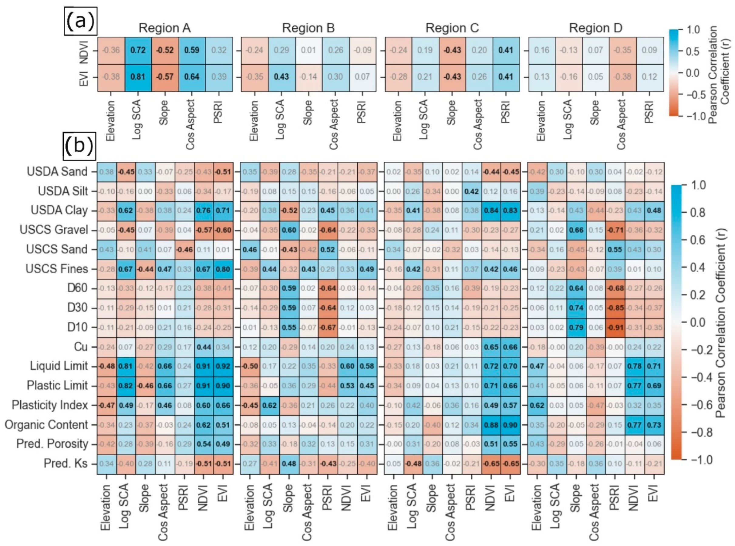
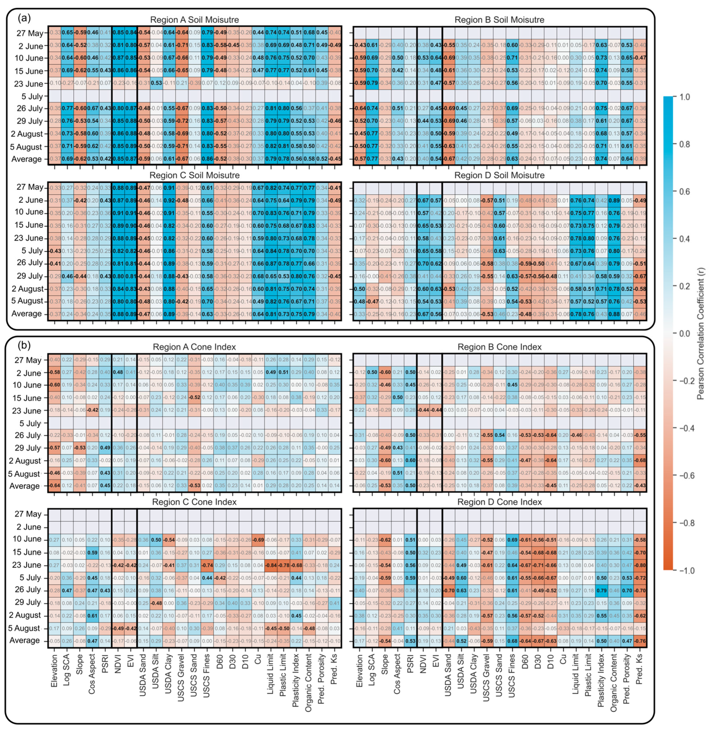
  • The strength of the relationships between soil moisture and topographic, vegetation, and soil composition attributes can vary substantially within a SMAP grid cell. Soil moisture is strongly correlated to topography in Region A and weakly correlated to topography in Region B but has few significant correlations with topography in Regions C and D. Soil moisture is strongly correlated to vegetation in Regions A and C, less correlated in Region D, and poorly correlated in Region B. Soil moisture is most correlated with soil attributes in Region A, followed by Regions C and D, with Region B having weak correlations.
  • The slopes of the relationships between soil moisture and topographic, vegetation, and soil composition attributes can also vary substantially within a SMAP grid cell. Region A has the greatest slopes for relationships between soil moisture and topography. Regions A and C have greater slopes for relationships of soil moisture with vegetation and soil than Regions B and D.
  • The strength of the relationships between soil strength and topographic, vegetation, and soil composition attributes can vary within a SMAP grid cell. Regions A, B, and D have weak correlations between soil strength and topography, while Region C has few significant correlations. Region D is the only region with consistent significant correlations between soil strength and compositional attributes.
Overall, the results contradict the assumption of homogeneous relationships that is typically applied when downscaling soil moisture. Thus, using constant parameters for soil moisture downscaling across the extent of a coarse-resolution grid cell may lead to suboptimal performance. Furthermore, because soil strength is influenced by soil moisture in unsaturated strength modeling procedures [3,7,72,73], modeled soil strength predictions may improve when soil moisture estimates from downscaling procedures consider the variability in the underlying relationships. Such improvements will be greater in cases where soil strength depends more strongly on soil moisture. Methods should be explored that cluster locations and infer separate parameters for those clusters. Machine learning methods that identify such clustering as part of their methodology are expected to outperform methods that implicitly assume consistent relationships across a coarse-resolution grid cell.
The degree of heterogeneity observed in this study region may not occur in other regions. For example, the study region has relatively homogeneous soils. Regions with more soil heterogeneity (e.g., diverse bedrock) may exhibit more heterogeneity in the soil moisture and strength relationships. Regions with more diverse landcover types may also demonstrate greater heterogeneity. The study also focused on summer conditions, when snow and frozen ground were absent. Spatial patterns of frozen ground, as well as snow redistribution, could produce different effects. Different summer seasons may also exhibit different behaviors due to alterations in space–time patterns of precipitation. Future studies should consider what combinations of factors (e.g., geology, soil parent material, soil depth, rockiness, vegetation type, vegetation density, topographic variability) determine the number and extent of clusters needed to characterize a given SMAP grid cell.

Supplementary Materials

The following supporting information can be downloaded at: https://www.mdpi.com/article/10.3390/hydrology12020034/s1, Figure S1: Maps of soil moisture for each sampling date; Figure S2: Maps of soil strength for each sampling date.

Author Contributions

Conceptualization, J.R.B., H.P., K.W., J.D.N., J.S.IV, and T.R.G.; methodology, J.R.B., H.P., K.W., J.D.N., J.S.IV, and T.R.G.; software, J.R.B. and H.P.; validation, J.R.B. and H.P.; formal analysis, J.R.B. and H.P.; investigation, J.R.B. and H.P.; resources, J.R.B., H.P., and K.W.; data curation, J.R.B. and H.P.; writing—original draft preparation, J.R.B. and H.P.; writing—review and editing, J.D.N., J.S.IV, and T.R.G.; visualization, J.R.B. and H.P.; supervision, J.D.N. and J.S.IV; project administration, J.D.N. and J.S.IV; funding acquisition, J.D.N., J.S.IV, and P.J.G. All authors have read and agreed to the published version of the manuscript.

Funding

This research was funded by the Army Research Laboratory and was accomplished under Cooperative Agreement Number W911NF-21-2-0252. The views and conclusions contained in this document are those of the authors and should not be interpreted as representing the official policies, either expressed or implied, of the Army Research Office or the U.S. Government. The U.S. Government is authorized to reproduce and distribute reprints for government purposes notwithstanding any copyright notation herein. Additional funding was provided by the National Science Foundation (2312319).

Data Availability Statement

Dataset available on request from the authors.

Acknowledgments

The authors gratefully acknowledge CSU STRATA and Joel Vaad for facilitating use of Maxwell Ranch for this research. The authors thank Sami Fischer, Matt Bullock, and Sam Jacob for their field data collection and Katie Ascough, Celie Brockett, Holly Ho, Kaylee Romero, and Alec Shields for their support in laboratory testing.

Conflicts of Interest

The authors declare no conflicts of interest.

Abbreviations

List of acronyms: AMSR-E, Advanced Microwave Scanning Radiometer for EOS; CH, high-plasticity clay; CL, low-plasticity clay; CI, cone index; Cu, coefficient of uniformity; D10, diameter at 10% mass finer; D30, diameter at 30% mass finer; D60, diameter at 60% mass finer; DEM, digital elevation model; EVI, enhanced vegetation index; Ks, saturated hydraulic conductivity; LL, liquid limit; MH, high-plasticity silt; ML, low-plasticity silt; NDVI, normalized difference vegetation index; OH, high-plasticity organic material; OL, low-plasticity organic material; p, Pearson statistical significance; PL, plastic limit; PI, plasticity index; PSRI, potential solar radiation index; RCI, rating cone index; RI, remold index; r, Pearson correlation coefficient; SCA, specific contributing area; SC-SM, silty clayey sand; SM, silty sand; SMAP, Soil Moisture Active Passive; SMOS, Soil Moisture Ocean Salinity; SP, poorly graded sand; SSURGO, Soil Survey Geographic Database; TauDEM, terrain analysis using digital elevation model; USCS, Unified Soil Classification System; USDA, United States Department of Agriculture; θ, surface soil moisture (cm3/cm3).

References

  1. Wulfsohn, D.; Adams, B.; Fredlund, D. Application of unsaturated soil mechanics for agricultural conditions. Can. Agric. Eng. 1996, 38, 173–181. [Google Scholar]
  2. Priddy, J.; Berney, E.; Peters, J. Effects of near-surface hydrology on soil strength and mobility. Geol. Soc. Lond. Spec. Publ. 2012, 362, 301–320. [Google Scholar] [CrossRef]
  3. Uusitalo, J.; Ala-Ilomäki, J.; Lindeman, H.; Toivio, J.; Siren, M. Modelling soil moisture–soil strength relationship of fine-grained upland forest soils. Silva Fenn. 2019, 53. [Google Scholar] [CrossRef]
  4. Schönauer, M.; Prinz, R.; Väätäinen, K.; Astrup, R.; Pszenny, D.; Lindeman, H.; Jaeger, D. Spatio-temporal prediction of soil moisture using soil maps, topographic indices, and SMAP retrievals. Int. J. Appl. Earth Obs. Geoinf. 2022, 108, 102730. [Google Scholar] [CrossRef]
  5. Fredlung, D. Unsaturated soil mechanics in engineering practice. J. Geotech. Geoenviron. Eng. 2006, 132, 286–321. [Google Scholar] [CrossRef]
  6. Stevens, M.; Towne, B.; Mason, G.; Priddy, J.; Osorio, J.; Barella, C. Procedure for One-Pass Vehicle Cone Index Determination for Acquisition Support; ERDC/GSL SR-13-2; US Army Corps of Engineers: Washington, DC, USA, 2013.
  7. Pauly, M.J. Modeling and Field Evaluation of Unsaturated Soil Strength for Vehicle Mobility. Master’s Thesis, Colorado State University, Fort Collins, CO, USA, 2019. [Google Scholar]
  8. Jurkat, M.P.; Nuttall, P.W.; Haley, P.W. The U.S. Army mobility model (AMM-75). In WES Papers from 5th International Conference International Society for Terrain-Vehicle Systems; Waterways Experiment Station: Vicksburg, MS, USA, 1975; pp. 5–52. [Google Scholar]
  9. Haley, P.W.; Jurkat, M.P.; Brady, P.M. NATO Reference Mobility Model, Edition I User’s Guide; Technical Report 12503; Tank-Automotive Research and Development Command: Warren, MI, USA, 1979. [Google Scholar]
  10. Ahlvin, R.B.; Haley, P.W. NATO Reference Mobility Model, Edition II User’s Guide; GL-92-19; Waterways Experiment Station: Vicksburg, MS, USA, 1992. [Google Scholar]
  11. McCoullough, M.; Jayakumar, P.; Dasch, J.; Gorsich, D. The next generation NATO reference mobility model development. J. Terramech. 2017, 73, 49–60. [Google Scholar] [CrossRef]
  12. Choi, K.K.; Gaul, N.; Jayakumar, P.; Wasfy, T.M. Framework of reliability-based stochastic mobility map for next generation NATO reference mobility model. J. Comput. Nonlinear Dynam. 2019, 14, 021012. [Google Scholar] [CrossRef]
  13. Gao, H.; Wood, E.F.; Jackson, T.J.; Drusch, M.; Bindlish, R. Using TRMM/TMI to retrieve surface soil moisture over the southern United States from 1998 to 2002. J. Hydrometeorol. 2006, 7, 23–38. [Google Scholar] [CrossRef]
  14. Wagner, W.; Hahn, S.; Kidd, R.; Melzer, T.; Bartalis, Z.; Hasenauer, S.; Figa-Saldaña, J.; de Rosnay, P.; Jann, A.; Schneider, S.; et al. The ASCAT soil moisture product: A review of its specifications, validation results, and emerging applications. Meteorol. Z. 2013, 22, 5–33. [Google Scholar] [CrossRef]
  15. Kachi, M.; Naoki, K.; Hori, M.; Imaoka, K. AMSR2 validation results. In Proceedings of the 2013 IEEE International Geoscience and Remote Sensing Symposium—IGARSS, Melbourne, VIC, Australia, 21–26 July 2013; pp. 831–834. [Google Scholar] [CrossRef]
  16. Kerr, Y.; Wigneron, J.; Delwart, S.; Cabot, F.; Boutin, J.; Escorihuela, M.; Font, J.; Reul, N.; Gruhier, C.; Juglea, S.; et al. The SMOS mission: New tool for monitoring key elements of the global water cycle. Proc. IEEE 2010, 98, 666–687. [Google Scholar] [CrossRef]
  17. O’Neill, P.; Entekhabi, D.; Njoku, E.; Kellogg, K. The NASA soil moisture active passive (SMAP) mission: Overview. In Proceedings of the 2010 IEEE International Geoscience and Remote Sensing Symposium, Honolulu, HI, USA, 25–30 July 2010; pp. 3236–3239. [Google Scholar] [CrossRef]
  18. Merlin, O.; Chebouni, A.G.; Kerr, Y.H.; Goodrich, D.C. A downscaling method for distributing surface soil moisture within a microwave pixel: Application to the monsoon ’90 data. Remote Sens. Environ. 2006, 101, 379–389. [Google Scholar] [CrossRef]
  19. Sadeghi, M.; Babaeian, E.; Tuller, M.; Jones, S.B. The optical trapezoid model: A novel approach to remote sensing of soil moisture applied to Sentinel-2 and Landsat-8 observations. Remote Sens. Environ. 2017, 198, 52–68. [Google Scholar] [CrossRef]
  20. Peng, J.; Loew, A.; Zhang, S.; Wang, J.; Niesel, J. Spatial downscaling of satellite soil moisture data using a vegetation temperature condition index. IEEE Trans. Geosci. Remote Sens. 2016, 54, 558–566. [Google Scholar] [CrossRef]
  21. Fang, B.; Lakshmi, V.; Bindlish, R.; Jackson, T. AMSR2 soil moisture downscaling using temperature and vegetation data. Remote Sens. 2018, 10, 1575. [Google Scholar] [CrossRef]
  22. Singh, A.; Gaurav, K. Deep Learning and Data Fusion to Estimate Surface Soil Moisture from Multi-Sensor Satellite Images. Sci. Rep. 2023, 13, 2251. [Google Scholar] [CrossRef] [PubMed]
  23. Fuentes, I.; Padarian, J.; Vervoort, R.W. Towards near Real-Time National-Scale Soil Water Content Monitoring Using Data Fusion as a Downscaling Alternative. J. Hydrol. 2022, 609, 127705. [Google Scholar] [CrossRef]
  24. Vergopolan, N.; Chaney, N.W.; Beck, H.E.; Pan, M.; Sheffield, J.; Chan, S.; Wood, E.F. Combining Hyper-Resolution Land Surface Modeling with SMAP Brightness Temperatures to Obtain 30-m Soil Moisture Estimates. Remote Sens. Environ. 2020, 242, 111740. [Google Scholar] [CrossRef]
  25. Coleman, M.L.; Niemann, J.D. Controls on topographic dependence and time-instability in catchment-scale soil moisture patterns. Water Resour. Res. 2013, 49, 1625–1642. [Google Scholar] [CrossRef]
  26. Ranney, K.J.; Niemann, J.D.; Lehman, B.M.; Green, T.R.; Jones, A.S. A method to downscale soil moisture to fine resolutions using topographic, vegetation and soil data. Adv. Water Resour. 2015, 76, 81–96. [Google Scholar] [CrossRef]
  27. Cowley, G.S.; Niemann, J.D.; Green, T.R.; Seyfried, M.S.; Jones, A.S.; Grazaitis, P.J. Impacts of precipitation and potential evapotranspiration patterns on downscaling soil moisture in regions with large topographic relief. Water Resour. Res. 2017, 53, 1553–1574. [Google Scholar] [CrossRef]
  28. Deshon, J.P.; Niemann, J.D.; Green, T.R.; Jones, A.S.; Grazaitis, P.J. Stochastic analysis and probabilistic downscaling of soil moisture in small catchments. J. Hydrol. 2020, 585, 124711. [Google Scholar] [CrossRef]
  29. Ali, G.; Roy, A.; Legendre, P. Spatial relationships between soil moisture patterns and topographic variables at multiple scales in a humid temperate forested catchment. Water Resour. Res. 2010, 46. [Google Scholar] [CrossRef]
  30. Mascaro, G.; Vivoni, E.; Deidda, R. Soil moisture downscaling across climate regions and its emergent properties. J. Geophys. Res. 2011, 116, 3128–3142. [Google Scholar] [CrossRef]
  31. Yu, B.; Liu, G.; Liu, Q.; Feng, J.; Wang, X.; Han, G.; Haung, C. Effects of micro-topography and vegetation type on soil moisture in a large gully on the Loess Plateau of China. Hydrol. Res. 2018, 46, 1255–1270. [Google Scholar] [CrossRef]
  32. Liang, W.; Li, S.; Hung, F. Analysis of the contributions of topographic, soil, and vegetation features on the spatial distributions of surface soil moisture in a steep natural forested headwater catchment. Hydrol. Process. 2017, 32, 3796–3809. [Google Scholar] [CrossRef]
  33. Mohanty, B.P.; Famiglietti, J.S.; Skaggs, T.H. Evolution of soil moisture spatial structure in a mixed vegetation pixel during the Southern Great Plains 1997 (SGP97) hydrology experiment. Water Resour. Res. 2000, 36, 3675–3686. [Google Scholar] [CrossRef]
  34. Western, A.; Zhou, S.; Grayson, R.; McMahon, T.; Bloschl, G.; Wilson, D. Spatial correlation of soil moisture in small catchments and its relationship to dominant spatial hydrological processes. J. Hydrol. 2004, 256, 113–134. [Google Scholar] [CrossRef]
  35. Lin, H.; Kogelmann, W.; Walker, C.; Burns, M. Soil moisture patterns in a forested catchment: A hydropedological perspective. Geoderma 2006, 131, 345–368. [Google Scholar] [CrossRef]
  36. Kim, S.; Heysun, L.; Woo, N.; Kim, J. Soil moisture monitoring on a steep hillside. Hydrol. Process. 2007, 21, 2823–2964. [Google Scholar] [CrossRef]
  37. Rosenbaum, U.; Bogena, H.R.; Herbst, M.; Huisman, J.A.; Peterson, T.J.; Weuthen, A.; Western, A.W.; Vereecken, H. Seasonal and event dynamics of spatial moisture patterns at the small catchment scale. Water Resour. Res. 2012, 48. [Google Scholar] [CrossRef]
  38. Fathololoumi, S.; Vaezi, A.R.; Firozjaei, M.K.; Biswas, A. Quantifying the effect of surface heterogeneity on soil moisture across regions and surface characteristic. J. Hydrol. 2021, 596, 126132. [Google Scholar] [CrossRef]
  39. Fischer, S.; Niemann, J.D.; Scalia, J.; Bullock, M.D.; Proulx, H.E.; Kim, B.; Green, T.R.; Grazaitis, P.J. Assessing the influence of model inputs on performance of the EMT+VS soil moisture downscaling model for a large foothills region in Northern Colorado. J. Hydrol. 2025, 650, 132397. [Google Scholar] [CrossRef]
  40. Chan, S.K.; Bindlish, R.; O’Neill, P.; Jackson, T.; Njoku, E.; Dunbar, S.; Kerr, Y. Development and assessment of the SMAP enhanced passive soil moisture product. Remote Sens. Environ. 2018, 204, 931–941. [Google Scholar] [CrossRef] [PubMed]
  41. O’Neill, P.E.; Chan, S.; Njoku, E.G.; Jackson, T.; Bindlish, R.; Chaubell, J.; Colliander, A. SMAP Enhanced L3 Radiometer Global and Polar Grid Daily 9 km EASE-Grid Soil Moisture, Version 5; NASA National Snow and Ice Data Center Distributed Active Archive Center: Boulder, CO, USA, 2021. [CrossRef]
  42. Western, A.W.; Grayson, R.B.; Blöschl, G.; Willgoose, G.R.; McMahon, T.A. Observed spatial organization of soil moisture and its relation to terrain indices. Water Resour. Res. 1999, 35, 797–810. [Google Scholar] [CrossRef]
  43. Wilson, D.J.; Western, A.W.; Grayson, R.B. A terrain and data-based method for generating the spatial distribution of soil moisture. Adv. Water Resour. 2005, 28, 43–54. [Google Scholar] [CrossRef]
  44. Perry, M.A.; Niemann, J.D. Generation of soil moisture patterns at the catchment scale by EOF interpolation. Hydrol. Earth Syst. Sci. 2008, 12, 39–53. [Google Scholar] [CrossRef]
  45. Eylander, J.; Bieszczad, J.; Ueckermann, M.; Peters, J.; Brooks, C.; Audette, W.; Ekegren, M. Geospatial weather affected terrain conditions and hazards (GeoWATCH) description and evaluation. Environ. Model. Softw. 2023, 160, 105606. [Google Scholar] [CrossRef]
  46. U.S. Geological Survey (USGS). USGS 1/3 Arc Second n41w106 20221118; U.S. Geological Survey: Reston, VA, USA, 2022.
  47. Tarboton, D.G. Terrain Analysis using Digital Elevation Models (TAUDEM). In Hydrology Research Group-Terrain Analysis Using Digital Elevation Models (Taudem); Utah State University: Logan, UT, USA, 2008. [Google Scholar]
  48. Lee, R. Potential insolation as a topoclimatic characteristic of drainage basins. Hydrol. Sci. J. 1964, 9, 27–41. [Google Scholar] [CrossRef]
  49. Swift, L.W., Jr. Algorithm for solar radiation on mountain slopes. Water Resour. Res. 1976, 12, 108–112. [Google Scholar] [CrossRef]
  50. Dingman, S.L. Physical Hydrology; Waveland Press: Long Grove, IL, USA, 1994; pp. 571–577. [Google Scholar]
  51. European Space Agency (ESA). Sentinel 2 MSI-Level 2A. Copernicus Open Access; European Space Agency: Paris, France, 2016. [Google Scholar]
  52. Kriegler, F.J.; Malila, W.A.; Nalepka, R.F.; Richardson, W. Preprocessing transformations and their effect on multispectral recognition. In Proceedings of the Sixth International Symposium on Remote Sensing of Environment, Ann Arbor, MI, USA, 13–16 October 1969; pp. 97–131. [Google Scholar]
  53. Liu, H.Q.; Huete, A. A Feedback based modification of the NDVI to minimize canopy background and atmospheric noise. IEEE Trans. Geosci. Remote Sens. 1995, 33, 457–465. [Google Scholar] [CrossRef]
  54. Huete, A.R.; Liu, H.Q.; Batchily, K.; van Leeuwen, W. A comparison of vegetation indices over a global set of TM images for EOS-MODIS. Remote Sens. Environ. 1997, 59, 440–451. [Google Scholar] [CrossRef]
  55. Soil Survey Staff, Natural Resources Conservation Service, United Stated Department of Agriculture. Web Soil Survey. Available online: http://websoilsurvey.nrcs.usda.gov/ (accessed on 1 July 2023).
  56. Stevens Water Monitoring System, Inc. Comprehensive Stevens HydraProbe User’s Manual; Stevens Water Monitoring System: Portland, OR, USA, 2018. [Google Scholar]
  57. Humboldt Mfg. Digital Proving Ring Penetrometer: Product Manual; Humboldt Mfg: Elgin, IL, USA, 2023. [Google Scholar]
  58. METER Group. PARIO User Manual V2017/12; METER Group AG: Munich, Germany, 2017. [Google Scholar]
  59. ASTM D7928-21; Standard Test Methods for Particle-Size Distribution (Gradation) of Soils Using the Sedimentation (Hydrometer) Analysis. American Society for Testing and Materials: West Conshohocken, PA, USA, 2021.
  60. Durner, W.; Iden, S.C.; von Unold, G. The integral suspension pressure method (ISP) for precise particle-size analysis by gravitational sedimentation. Water Resour. Res. 2017, 53, 33–48. [Google Scholar] [CrossRef]
  61. ASTM D6913/D6913M-17; Standard Test Methods for Particle-Size Distribution (Gradation) of Soils Using Sieve Analysis. American Society for Testing and Materials: West Conshohocken, PA, USA, 2017.
  62. Cosby, B.J.; Hornberger, G.M.; Clapp, R.B.; Ginn, T.R. A statistical exploration of the relationships of soil-moisture characteristics to the physical properties of soils. Water Resour. Res. 1984, 20, 682–690. [Google Scholar] [CrossRef]
  63. United States Department of Agriculture (USDA). Soil Taxonomy: A Basic System of Soil Classification for Making and Interpreting Soil Surveys; Government Printing Office: Washington, DC, USA, 1975.
  64. ASTM D4318-17e1; Standard Test Methods for Liquid Limit, Plastic Limit, and Plasticity Index of Soils. American Society for Testing and Materials: West Conshohocken, PA, USA, 2010.
  65. ASTM D2487-17e1; Standard Practice for Classification of Soils for Engineering Purposes (Unified Soil Classification System). American Society for Testing and Materials: West Conshohocken, PA, USA, 2017.
  66. ASTM D2974-20e1; Standard Test Methods for Determining the Water (Moisture) Content, Ash Content, and Organic Material of Peat and Other Organic Soils. American Society for Testing and Materials: West Conshohocken, PA, USA, 2020.
  67. Rezanezhad, F.; Price, J.S.; Quinton, W.L.; Lennartz, B.; Milojevic, T.; Van Cappellen, P. Structure of peat soils and implications for water storage, flow and solute transport: A review update for geochemists. Chem. Geol. 2016, 429, 75–84. [Google Scholar] [CrossRef]
  68. Casagrande, A. Classification and identification of soils. Trans. Am. Soc. Civil Eng. 1948, 113, 901–930. [Google Scholar] [CrossRef]
  69. Brooks, R.H.; Corey, A.T. Hydraulic Properties of Porous Media; Hydrology Papers; Colorado State University: Fort Collins, CO, USA, 1964. [Google Scholar]
  70. van Genuchten, M.T.; Leij, F.J.; Yates, S.R. The RETC Code for Quantifying the Hydraulic Functions of Unsaturated Soils; U.S. Salinity Laboratory, U.S. Department of Agriculture, Agricultural Research Service: Riverside, CA, USA, 1991. [Google Scholar]
  71. Moeslund, J.; Arge, L.; Bocher, P.; Dalgaard, T.; Odgaard, M.; Nygaard, B.; Svenning, J. Topographically controlled soil moisture is the primary driver of local vegetation patterns across a lowland region. Ecosphere 2013, 4, 1–26. [Google Scholar] [CrossRef]
  72. Fredlund, D.G.; Morgenstern, N.R.; Widger, R.A. The shear strength of unsaturated soils. Can. Geotech. J. 1978, 15, 313–321. [Google Scholar] [CrossRef]
  73. Lu, N.; Godt, J.; Wu, D. A closed-form equation for effective stress in variably saturated soil. Water Resour. Res. 2010, 46. [Google Scholar] [CrossRef]
Figure 1. (a) Map of Maxwell Ranch, including ranch boundary, study regions, weather station, and sampling locations (map extent corresponds to a SMAP 9 km grid cell); (be) maps of Regions A, B, C, and D with corresponding sampling locations and photos at each region.
Hydrology 12 00034 g001
Figure 2. Daily precipitation, average soil moisture from field measurements (labeled HydraProbe), and SMAP for sampling dates in 2022. SMAP soil moisture was determined using the Enhanced Level 3 Radiometer data product [40,41]. SMAP data were unavailable for 27 May. Precipitation data were recorded by the KCOLIVER 12 weather station.
Hydrology 12 00034 g002
Figure 3. Maps of (a) elevation, (b) cos(aspect), (c) slope, (d) log SCA, (e) PSRI, (f) NDVI, (g) EVI, (h) SSURGO percentage of sand, (i) SSURGO percentage of silt, and (j) SSURGO percentage of clay along with sampling locations and ranch boundary.
Hydrology 12 00034 g003
Figure 4. Histograms of the topographic, vegetation, and soil attributes for the SMAP grid cell (unhatched bars) and the sampling locations (hatched bars). Histograms include (a) elevation, (b) cos(aspect), (c) slope, (d) log SCA, (e) PSRI, (f) NDVI, (g) EVI, (h) SSURGO percentage of sand, (i) SSURGO percentage of silt, and (j) SSURGO percentage of clay.
Hydrology 12 00034 g004
Figure 5. (a) USDA soil texture classification for all sampling locations; (b) Atterberg limit summary for all sampling locations where CL is low-plasticity clay, ML is low-plasticity silt, CH is high-plasticity clay, MH is high-plasticity silt, OL is low-plasticity organic material, and OH is high-plasticity organic material.
Hydrology 12 00034 g005
Figure 6. Maps of soil moisture for each sampling region on a representative dry date (23 June) and a wet date (29 July). Symbols represent sampling locations, and infill colors indicate measured soil moisture.
Hydrology 12 00034 g006
Figure 7. Histograms of the soil moisture measurements collected in each sampling region on each sampling date including (a) 27 May, (b) 2 June, (c) 10 June, (d) 15 June, (e) 23 June, (f) 5 July, (g) 26 July, (h) 29 July, (i) 2 August, (j) 5 August. Spatial average soil moisture ( θ ¯ ; cm3/cm3) for entire site and each sampling study region are shown in the subplots. Soil moisture was not measured for all regions on 27 May and 5 July due to lightning hazard.
Hydrology 12 00034 g007
Figure 8. Maps of soil strength (viz. CI) for each region on a representative dry date (23 June) and a wet date (29 July). Symbols represent sampling locations, and infill color indicates measured CI.
Hydrology 12 00034 g008
Figure 9. Histograms of soil strength (viz. CI) measurements collected at each sampling location for each sampling date including (a) 27 May, (b) 2 June, (c) 10 June, (d) 15 June, (e) 23 June, (f) 5 July, (g) 26 July, (h) 29 July, (i) 2 August, (j) 5 August. Average CI for the entire study site and each study region are shown within the subplots. CI was not measured at all locations on 27 May, 2 June, and 5 July due to lightning hazard.
Hydrology 12 00034 g009
Figure 10. (a) Pearson correlations of vegetation indices with topographic attributes for each region and (b) Pearson correlations of soil attributes with topographic and vegetation indices for each region. Correlations displayed with bold black text represent statistically significant correlations based on the Pearson p-value (p < 0.05). Other correlations are displayed in grey text.
Hydrology 12 00034 g010
Figure 11. Pearson correlations of (a) soil moisture and (b) soil strength with topography, vegetation, and soil attributes for each region. Correlations displayed with bold black text represent statistically significant correlations based on the Pearson p-value (p < 0.05). Other correlations are displayed in grey text.
Hydrology 12 00034 g011
Figure 12. Ratio of the slope calculated in each sampling region to the slope calculated for the complete dataset for (a) soil moisture and (b) soil strength. Ratios are shown only for correlations that are significant in more than one region.
Hydrology 12 00034 g012
Disclaimer/Publisher’s Note: The statements, opinions and data contained in all publications are solely those of the individual author(s) and contributor(s) and not of MDPI and/or the editor(s). MDPI and/or the editor(s) disclaim responsibility for any injury to people or property resulting from any ideas, methods, instructions or products referred to in the content.

