Article

Spatiotemporal Modeling of Surface Water–Groundwater Interactions via Multi-Task Transformer-Based Learning

by
Hao Jing
1,2,
Yong Tian
2,3 and
Chunmiao Zheng
2,4,*
1
School of Environment, Harbin Institute of Technology, Harbin 150001, China
2
Guangdong-Hong Kong Joint Laboratory for Soil and Groundwater Pollution Control, School of Environmental Science & Engineering, Southern University of Science and Technology, Shenzhen 518055, China
3
State Key Laboratory of Soil Pollution Control and Safety, School of Environmental Science & Engineering, Southern University of Science and Technology, Shenzhen 518055, China
4
School of the Environment and Sustainable Engineering, Eastern Institute of Technology, Ningbo 315200, China
*
Author to whom correspondence should be addressed.
Hydrology 2025, 12(11), 291; https://doi.org/10.3390/hydrology12110291 (registering DOI)
Submission received: 21 September 2025 / Revised: 29 October 2025 / Accepted: 31 October 2025 / Published: 2 November 2025
(This article belongs to the Topic Advances in Groundwater Science and Engineering)

Abstract

A spatiotemporal, multi-task learning (MTL) model for simulating surface water–groundwater (SW-GW) dynamics is developed and applied to the Heihe River Basin, Northwest China. The Transformer-based model (MT-TFT) jointly forecasts surface runoff and groundwater levels, outperforming MTL models built on gated recurrent unit (GRU) and long short-term memory (LSTM) architectures. Compared with single-task learning, adding a coupled groundwater-level task markedly improves surface runoff prediction, achieving a Nash–Sutcliffe efficiency (NSE) of 0.73 and a coefficient of determination (R2) of 0.75. Attention-based interpretability shows that the model assigns the highest weights to time steps with elevated precipitation; as lead time shortens, attention further concentrates on these periods, improving the accuracy of near-term, multi-step forecasts. These results highlight the value of inductive transfer across hydrologic targets and demonstrate that MT-TFT provides an effective, interpretable framework for SW–GW coupling.

1. Introduction

As a critical component of the world’s water resources, groundwater serves as a major source of supply for domestic, industrial, and agricultural water use [1,2]. Statistics indicate that agricultural irrigation accounts for approximately 90% of global water consumption [3,4,5], of which about 40% is derived from groundwater [6]. Consequently, groundwater plays a pivotal role in ensuring global food security [2]. However, groundwater resources around the globe are exceedingly fragile, due to a variety of interconnected factors, such as climate change, anthropogenic and geogenic contamination, and overconsumption [7,8]. On the one hand, climate change alters groundwater system dynamics by modifying hydrological factors such as runoff and soil moisture. In turn, changes in groundwater dynamics affect terrestrial energy and moisture cycles through processes such as evapotranspiration, thereby contributing feedback to climate change [2,5]. On the other hand, rapid socioeconomic development and expanding populations have markedly increased groundwater demand, and large-scale extraction has directly reduced groundwater storage. A series of acute resource and environmental problems observed worldwide are closely associated with groundwater. Decades of intensive exploitation have cumulatively degraded both its quality and quantity, resulting in depletion and triggering severe environmental and geological consequences such as land subsidence, water quality deterioration, seawater intrusion, and ecosystem shrinkage [9,10,11,12].
Accurately characterizing changes in groundwater dynamics and forecasting groundwater conditions under various scenarios requires high-quality data support. In recent years, rapid advances in the Internet of Things (IoT)-based groundwater monitoring systems, sensor technology, 5G communications, and cloud computing have ushered groundwater sustainability management into the era of big data [13]. Despite the enormous potential of big data, the limitations of traditional groundwater management and analysis techniques in processing such data have created an urgent need for methodological and technological innovations. The recent surge of artificial intelligence—with machine learning and deep learning at the forefront—has demonstrated remarkable capabilities in processing and analyzing complex, high-dimensional datasets.
Previous studies on surrogate models for groundwater have largely concentrated on applying machine learning algorithms to simulate and forecast the spatiotemporal dynamics of groundwater systems [14,15,16,17,18,19]. Building on these findings, the present study focuses on the coupling simulation of surface water–groundwater systems. In integrated watershed water resource management, it is imperative to consider surface water and groundwater as a unified system and to accurately capture the interaction between them. Consequently, coupled surface water–groundwater models have emerged as a new trend in the development of watershed management models [20].
While process-based coupled surface water–groundwater models (exemplified by ParFlow and HeiFlow) have been extensively investigated, few studies have reported the use of machine learning algorithms as surrogate models for such coupling simulations. Previous research [21,22,23,24] has demonstrated that machine learning can achieve high accuracy in simulating and predicting the spatiotemporal dynamics of groundwater by effectively capturing latent relationships among hydrological, meteorological, and other driving factors. In the domain of surface runoff simulation, deep learning architectures such as long short-term memory (LSTM) and gated recurrent unit (GRU) networks have been applied within precipitation–runoff modeling systems (PRMSs) to model complex non-linear hydrological processes. For instance, Jiang et al. [25] employed a hybrid convolutional neural network–long short-term memory (CNN–LSTM) model to simulate the precipitation–runoff process in the Heihe River Basin (HRB), Northwestern China, achieving promising results. Building on the demonstrated capability of deep learning algorithms to independently model surface water and groundwater, the present study investigates their potential for application in the coupled simulation of surface water–groundwater systems.
The HRB, a typical inland river basin in China, exhibits pronounced water conflicts in its middle and lower streams and a more complex water cycle compared to the North China Plain [26], where surface runoff is relatively scarce. These characteristics result in intricate interactions between surface water and groundwater, making the HRB an exemplary region for investigating such processes. Unlike the work of Jing et al. (2023) [27], which focused on the North China Plain to evaluate deep learning approaches for simulating groundwater spatiotemporal dynamics, the present study selects the middle streams of the HRB as the research area. Here, the coupled simulation of surface water and groundwater is formulated as a multi-task modeling problem, where one task involves simulating precipitation–runoff processes (surface water) and the other addresses the spatiotemporal dynamics of groundwater. Building on the groundwater spatiotemporal dynamics model developed by Jing et al. (2023) [27] under a multi-task learning framework, this study constructs a coupled surface water–groundwater simulation model within the same paradigm. The specific objectives are to (a) compare the performance of different deep learning algorithms—gated recurrent unit (GRU), long short-term memory (LSTM), and Transformer architectures—as base models in a multi-task framework for coupled surface water–groundwater simulation; (b) contrast these results with those from single-task models (i.e., independent precipitation–runoff and groundwater models) to identify the optimal coupled model configuration under multi-task learning; and (c) improve model interpretability by analyzing influencing factors using techniques such as Self-Organizing Maps (SOMs) and self-attention mechanisms.

2. Materials and Methods

2.1. Study Area

The Heihe River Basin (HRB), located in the arid region of Northwest China, is the second-largest inland river basin in China, extending between 97.1–102.0° E and 37.7–42.7° N, and covering approximately 143,000 km2 (Figure 1). Topographically, the upstream is dominated by the Qilian Mountains, with rugged terrain and elevations ranging from 3000 m to 5500 m. The middle streams form a corridor between the Qilian Mountains and the Longshou Mountains, extending ~350 km east–west and 20–50 km north–south. Elevations here generally range from 1400 m to 1700 m, decreasing from south to north and from west to east, producing distinct vertical and horizontal gradients in climate and hydrology.
The hydrogeological setting of the basin shows clear spatial heterogeneity in both lithology and structure. In the middle oasis basin, located between the mountain front and the foreland of the alluvial fan, rivers have deposited large amounts of coarse-grained materials, creating favorable conditions for groundwater storage. The uplift of the Qilian Mountains led to the accumulation of alluvial fan and fluvial deposits, which mainly consist of unconsolidated Quaternary sediments. These deposits exhibit a south–north transition, with coarse gravels in the south gradually grading into medium- to fine-grained sands and silts toward the north [28,29,30].
In the mountainous upper streams of the HRB, the groundwater system is primarily recharged by rainfall infiltration. In the alluvial plain of the HRB’s middle streams, groundwater systems are closely connected with surface rivers. Under the combined influence of climate change and irrigation practices, the exchange fluxes between surface water and groundwater exhibit pronounced seasonal patterns, while these factors further modulate evapotranspiration processes. In the downstream desert region, groundwater levels constitute a critical factor influencing desert vegetation growth, as groundwater directly supports plant evapotranspiration, thereby sustaining the ecosystem of this arid river basin [31,32,33,34].

2.2. Simulation Target and Hydrological Inputs

(1) Groundwater-level and streamflow data
Historical groundwater-level (GWL) and streamflow data in HRB were obtained from the Water Resources Department of Gansu Province. The GWL dataset comprises 25 observation wells collected between 2001 and 2012 (Figure 1). The streamflow dataset contains the daily streamflow collected at the Yingluo gauging station between 2001 and 2012. A Self-Organizing Map (SOM) algorithm was used to cluster the spatiotemporal variations in groundwater dynamics in the middle streams of the HRB.
(2) China Meteorological Forcing Dataset
Meteorological inputs were sourced from the China Meteorological Forcing Dataset, which integrates multiple observational and reanalysis products. China Meteorological Forcing Data (CMFD) is a high-precision, high-resolution, and long-time-series dataset developed to support research in the fields of land surface, hydrology, and ecology over China. The CMFD dataset is created by integrating conventional meteorological observation data from the China Meteorological Administration with background fields from GLDAS, GEWEX-SRB, and TRMM [35,36,37]. The dataset spans 1979–2010, with a spatial resolution of 0.1° and a temporal resolution of 3 h. It is widely used in hydrological modeling, land surface modeling, land data assimilation, and other terrestrial applications. Since the simulation targets in this study (groundwater level and streamflow) are available only for the period 2001–2012, we selected the corresponding time range of the forcing data (temperature, wind speed, and precipitation). All detailed dataset information are summarized in Table 1.

2.3. Conceptual Model of Surface Water–Groundwater Coupling in the HRB

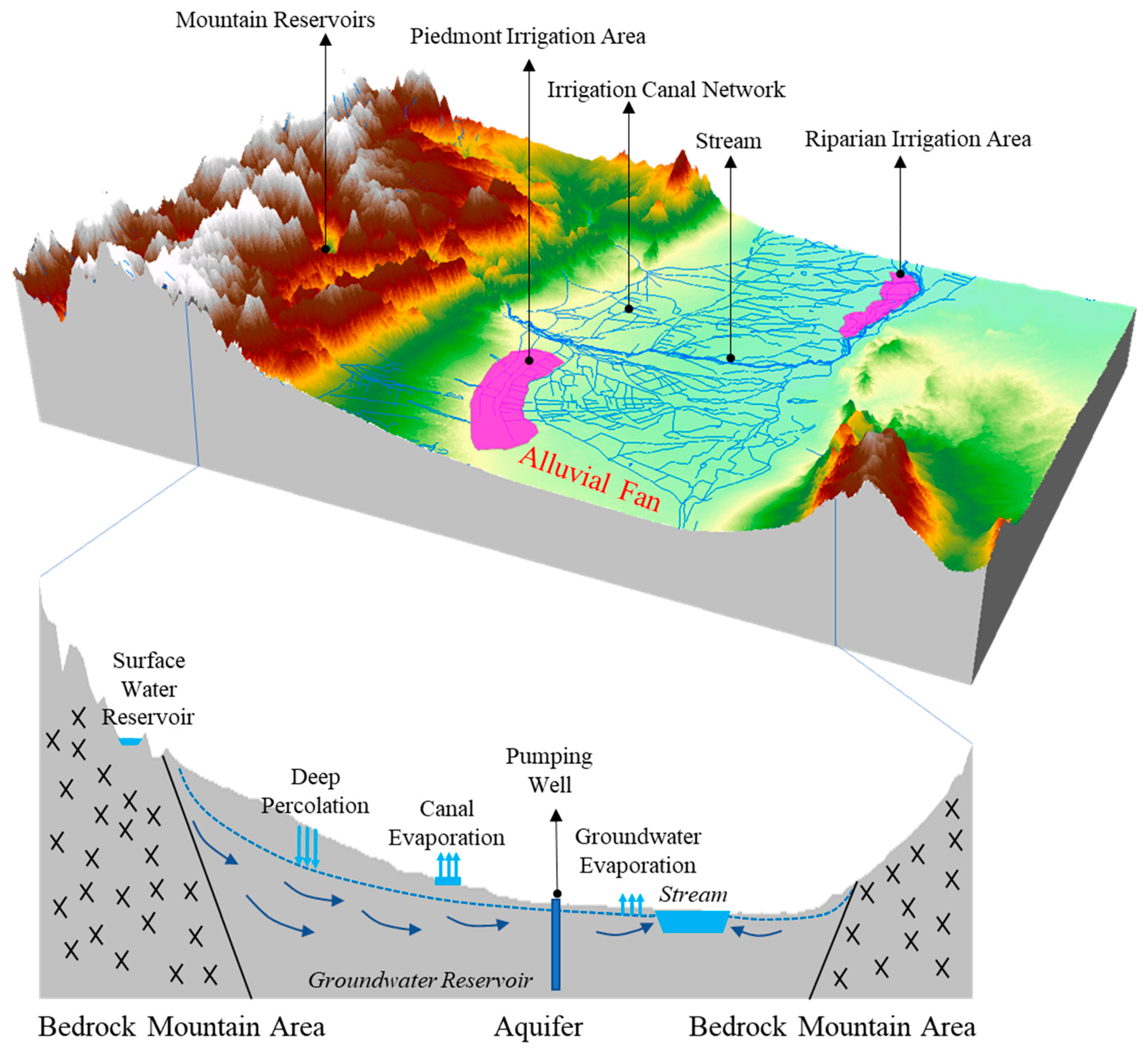
In the middle streams of the HRB, surface water–groundwater interactions are highly complex. Drawing on the work of Yao et al. (2015, 2018) [38,39], this study develops a conceptual framework (Figure 2) encompassing two primary subsystems—surface land processes and groundwater flow processes—linked through five core elements of the hydrological cycle: atmosphere, soil zone, surface runoff, vadose zone, and saturated zone.
The atmosphere represents the main climatic drivers, including precipitation, temperature, and solar radiation. The surface land processes are mainly based on the rainfall–runoff process model, including atmospheric precipitation, evapotranspiration, vegetation canopy interception, surface runoff, soil moisture movement, interflow, and groundwater infiltration recharge. The groundwater flow processes mainly include vertical water flow processes in the vadose zone, groundwater flow processes in the saturated zone, and the interaction processes between groundwater and surface water (river infiltration and groundwater discharge).
Many interaction components—such as interflow, river infiltration, and groundwater discharge—lack long-term direct measurements. Available multi-year datasets primarily include hydrometeorological variables (precipitation, temperature, solar radiation, and evapotranspiration) from remote sensing and reanalysis products, as well as surface runoff and groundwater-level dynamics from observation stations.
In this study’s supervised deep learning framework, long-term meteorological inputs and underlying surface characteristics (e.g., elevation and slope) derived from remote sensing serve as model drivers, while observed surface runoff and groundwater levels are used as target variables for coupled simulation of surface water–groundwater processes in the middle HRB.

2.4. Construction of a Coupled Surface Water–Groundwater Model Based on a Multi-Task Learning Framework

2.4.1. Multi-Task Learning Framework

Multi-task learning (MTL) is a deep learning strategy designed to improve overall model performance by simultaneously learning multiple related tasks. Unlike single-task learning (STL), MTL shares low-level features across tasks and exploits their mutual dependencies to enhance generalization and learning efficiency [40]. This approach improves data utilization, mitigates overfitting, and can accelerate convergence for related or downstream tasks. The central principle of MTL is to capture task correlations through shared representations, thereby improving generalizability across domains.
The MTL architecture typically comprises two components [41]: shared layers and task-specific layers. The shared layers, located at the lower levels of the network, are responsible for learning general, task-independent features through parameter sharing. By sharing parameters, these layers enable the model to better capture the overall characteristics of the input data. The task-specific layers, above the shared layers, are dedicated to extracting features pertinent to each individual task.
In MTL, there are generally two types of task sharing: (1) Hard Parameter Sharing is where hidden layers are shared across tasks, with separate output layers for each. This approach reduces model complexity and overfitting risk. (2) Soft Parameter Sharing is where each task has its own model, but parameters are regularized to encourage similarity.
In this study, the performance of different deep learning algorithms—namely the gated recurrent unit (GRU), long short-term memory (LSTM) network, and Transformer architecture—was compared when they were employed as backbone models within a multi-task learning framework for the simulation of coupled surface water–groundwater processes. All three models are well suited for time-series prediction tasks: GRU is computationally efficient and effective for shorter sequences, LSTM excels at capturing long-term dependencies, and the Transformer, through its attention mechanism, is particularly powerful in modeling complex, long-range interactions across multiple variables. The MTL models were further benchmarked against STL counterparts, including a standalone rainfall–runoff model and a groundwater spatiotemporal dynamics model, and their relative predictive capabilities were evaluated. Through this comparative analysis, optimal strategies for constructing high-performance coupled surface water–groundwater models under a multi-task learning paradigm were explored. In the following sections, detailed descriptions are provided for MTL architectures based on recurrent neural networks (represented by GRU and LSTM) and on the Transformer architecture.

2.4.2. Multi-Task Learning Framework Based on Recurrent Neural Networks

Recurrent neural networks (RNNs) have been widely adopted for hydrological and environmental modeling due to their capability to capture sequential dependencies and temporal dynamics in time-series data [42]. Within this family, the LSTM network [43] and GRU network [44] are two representative architectures that effectively address the vanishing gradient problem and enable the modeling of long-term temporal dependencies [45].
The LSTM is a prominent variant of the RNN architecture, designed to address sequence modeling tasks and capture temporal dynamics in data. Similar to conventional RNNs, LSTM networks are capable of processing sequential information; however, their specialized gating mechanisms enable the retention and propagation of long-term dependencies across time steps. This design effectively mitigates the vanishing gradient problem commonly encountered in traditional RNNs and enhances the model’s ability to learn long-range temporal correlations. Originally proposed by Hochreiter and Schmidhuber in 1997 [35], LSTM has since become a foundational technique in various domains, including natural language processing, speech recognition, and time-series forecasting.
The GRU is a variant of the RNN architecture, introduced by Cho et al. in 2014 [36], designed to address the vanishing gradient problem and the challenges of modeling long-term dependencies in sequential data. The core mechanism of GRU involves two gating components—the update gate and the reset gate—which regulate the flow of information and enable the network to learn and retain long-range temporal dependencies more effectively. Specifically, the update gate determines the extent to which the hidden state from the previous time step is preserved, while the reset gate controls whether the previous hidden state should be reset. One of GRU’s key advantages over the traditional LSTM network lies in its simplified structure, with fewer gating units and parameters, resulting in reduced computational complexity. The detailed mathematical equations about LSTM and GRU are reported in the Supplementary Materials.
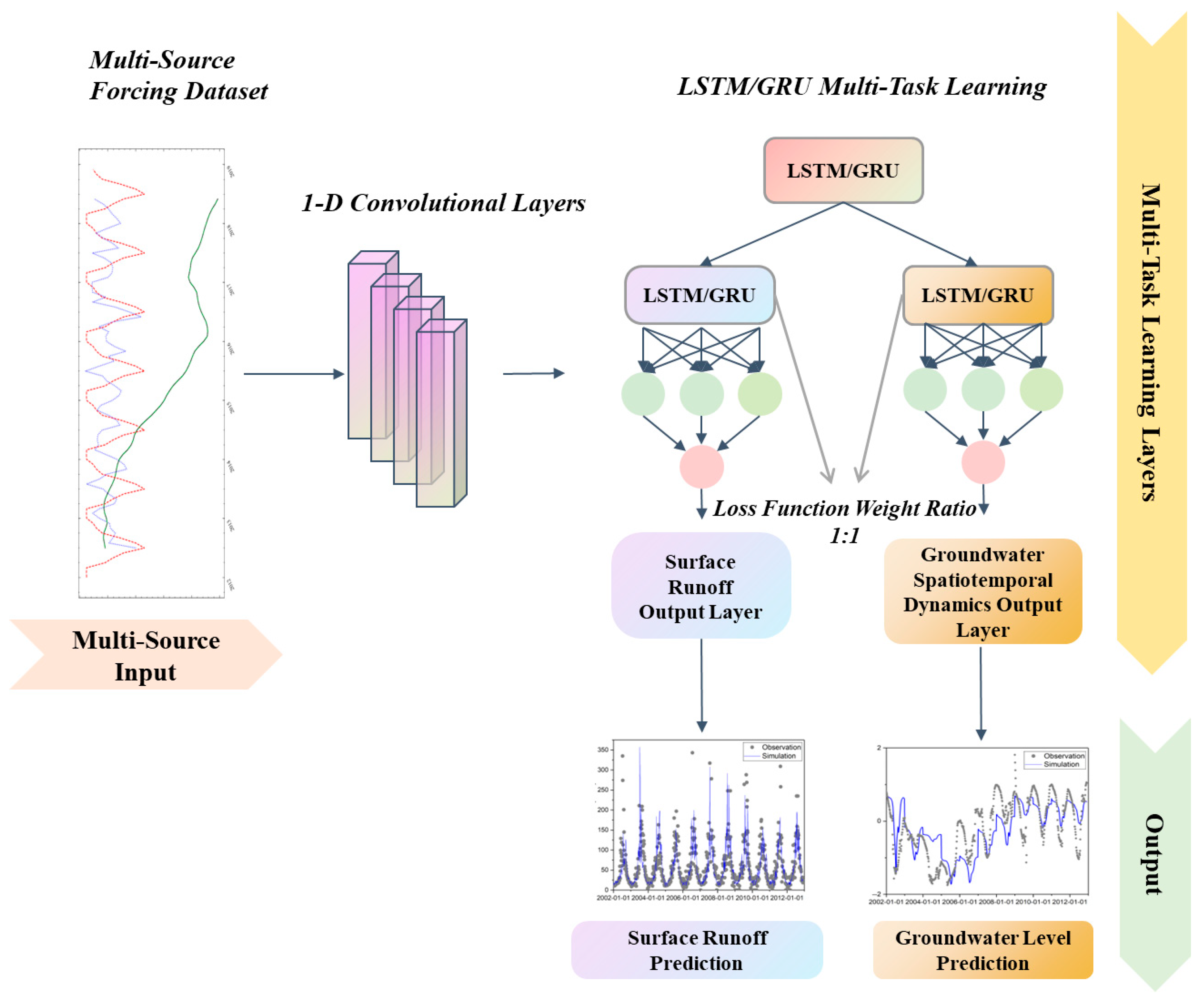
In the proposed MTL framework, these RNN-based architectures were selected as the temporal modeling components. The MTL framework proposed here integrates three deep learning architectures: convolutional neural networks (CNNs) [46], LSTM, and GRU. The model design (Figure 3) combines one-dimensional CNNs (1D-CNNs) with LSTM or GRUs to exploit their complementary strengths—CNNs for hierarchical spatial feature extraction and recurrent units for capturing long-range temporal dependencies in hydrological processes.
Meteorological, runoff, and groundwater spatiotemporal data are first processed by a shared 1D-CNN layer, in which high-dimensional spatial features are hierarchically extracted. These features are then passed to a second shared layer composed of either LSTM or GRU networks, where coupled temporal variation patterns between groundwater dynamics and river runoff are captured. Subsequently, two task-specific recurrent modules (LSTM or GRU) further refine temporal representations for groundwater-level dynamics and surface runoff, respectively, before fully connected layers generate the final predictions.
Model training is guided by the coefficient of determination (R2) as the loss function for both tasks, with equal weighting (1:1) applied during backpropagation to ensure balanced optimization. Through this design, CNNs provide robust spatial feature extraction, while LSTM and GRU networks effectively model long-term temporal dependencies—capabilities essential for accurately representing the dynamic interactions within coupled surface water–groundwater systems.

2.4.3. Multi-Task Learning Framework Based on Temporal Fusion Transformer

In this study, the Temporal Fusion Transformer (TFT) model developed by Lim et al. (2021) [47] is adopted as an interpretable, multivariate time-series forecasting approach within a multi-task learning framework for regional surface water–groundwater coupling simulation. TFT combines the representational capacity of the Transformer architecture with components specifically designed for time-series analysis, enabling the explicit integration of temporal variations and contextual information from historical observations to produce multi-horizon forecasts [48,49,50,51,52]. Its key advantages include (1) a Transformer-based self-attention mechanism that captures long-range dependencies in the input sequence—an approach widely used in natural language processing and increasingly in time-series analysis, yet rarely explored in hydrology and groundwater studies; (2) an interpretable fusion mechanism that integrates diverse temporal and contextual features to enhance model transparency; (3) a multi-step forecasting design optimized for simultaneous prediction of multiple future time points; and (4) the generation of probabilistic forecasts alongside point estimates, allowing uncertainty quantification and improving the reliability of simulation outputs.
The overall TFT architecture (Figure 4) comprises a Gated Residual Network (GRN), Variable Selection Network (VSN), Static Covariate Encoders (SCEs), Temporal Fusion Decoder (TFD), Static Enrichment Layer (SEL), Temporal Self-Attention Layer (TSL), and Position-wise Feed-forward Layer (PFL). The detailed mathematical information can be found at [47].
The GRN module regulates the contribution of each driving input variable to the model’s predictions. In regional surface water–groundwater simulations, complex, potentially non-linear relationships often exist between heterogeneous drivers—such as precipitation, temperature, and wind speed—and target variables, including groundwater-level dynamics and surface runoff. The degree of non-linear transformation required is generally unknown a priori. For instance, in basins with simple rainfall–runoff regimes, meteorological variables (e.g., precipitation) may exhibit near-linear relationships with runoff. Conversely, in catchments with intricate land–surface and groundwater interactions, the model’s capacity to represent non-linear dependencies critically affects predictive performance. The GRN addresses this by adaptively modulating non-linear processing through gating mechanisms. The governing equations are given as follows [47]:
G L U ( X ) = σ ( W 1 X + b 1 ) ( W 2 X + b 2 )
G R N ( a , c ) = L a y e r N o r m ( a + G L U ( η 1 ) )
η 1 = W 3 η 2 + b 3
η 2 = E L U ( W 4 a + W 5 c + b 4 )
where E L U is the Exponential Linear Unit activation function, G L U denotes the gated linear units, X is the input to the gated linear unit, W 1 , W 2 , W 3 , W 4 , and W 5 are the learnable weight matrix parameters, b 1 , b 2 , b 3 ,   a n d   b 4 are the corresponding bias parameters, σ is the Sigmoid activation function, a and c are the inputs to the G R N , with a considered as the main input and c as the optional input vector, η 1   and   η 2 are the intermediate layers, represents the element-wise (Hadamard) product, and L a y e r N o r m is the standard layer normalization.
The VSN assigns a dedicated variable selection unit to each category of input—namely, static covariates, historical observations, and known future inputs. Through end-to-end training, it learns a set of importance weights that quantify the predictive contribution of each feature, thereby performing an initial screening of input variables before further processing by downstream modules. Formally, the variable selection operation can be expressed as follows [47]:
VS ( x ) = softmax ( W s x + b s ) x
where VS ( x ) is the Variable Selection Network, W s denotes the learnable weight matrix parameters, b s denotes the corresponding bias parameters, x is the input to the Variable Selection Network, represents the element-wise (Hadamard) product, and softmax is the activation function.
The Temporal Fusion mechanism uses an interpretable self-attention layer to learn long-term dependencies. The attention weights in the TFT are central to its ability to perform interpretable multi-horizon time-series forecasting. They allow the model to adaptively select relevant time steps, input features, and temporal patterns across different prediction horizons. The formula for self-attention can be expressed as follows [47]:
Attention ( Q , K , V ) = softmax ( Q K T d k ) V
where Q , K , and V are the query, key, and value, respectively, and d k represents the dimension of the key.

2.5. Self-Organizing Map (SOMs)

The Self-Organizing Map (SOM), also known as the Kohonen network, is an unsupervised artificial neural network designed to project high-dimensional data onto a lower-dimensional space (typically two-dimensional) while preserving the topological relationships of the input data. Proposed by Teuvo Kohonen in 1982 [53], SOM emulates the self-organizing properties of the biological brain to achieve feature mapping and pattern recognition. Its core principle is to cluster similar input patterns onto adjacent nodes in the network through a self-organizing learning process. The network architecture consists of a two-dimensional (or higher-dimensional) grid, where each node represents a weight vector, collectively forming the SOM output layer. During training, input patterns are processed through competitive learning and weight adaptation, whereby the node most similar to the input—termed the Best Matching Unit (BMU)—is identified, and the weights of both the BMU and its neighboring nodes are updated, progressively forming a topological mapping of the data.
SOM training comprises two stages: initialization and iterative adaptation. In the initialization stage, each neuron in the competitive layer is assigned a weight vector with small random values, representing a point in the input space. In the iterative stage, node weights are progressively adjusted based on input patterns to establish topological relationships. This process involves four key steps: (1) initialization—weight vectors of competitive layer neurons are initialized with small random values; (2) competition—for each input vector, distances to all neuron weight vectors are computed, and the neuron with the smallest distance is selected as the BMU; (3) cooperation—the neighborhood of the BMU is determined, and the weights of neurons within this neighborhood are updated; and (4) adaptation—the weights of the BMU and its neighbors are adjusted according to the learning rate and neighborhood function, moving them closer to the current input vector.
A distinctive feature of SOM is its ability to preserve the topological structure of the input space while mapping it to a low-dimensional output space. This capability enables SOM to perform both clustering analysis and visualization of high-dimensional data. Similar input patterns are mapped to adjacent positions in the output layer, forming clusters that reveal intrinsic data structures. The method requires no labeled data, allowing for automatic clustering and pattern recognition, and is well suited for exploratory data analysis. Moreover, SOM exhibits strong generalization ability, enabling the recognition of previously unseen input samples.
In this study, given the high temporal complexity of groundwater observation data, the SOM was employed to perform unsupervised clustering analysis of groundwater observations in the HRB, providing a data foundation for subsequent result interpretation.

2.6. Experimental Design

For model input, meteorological drivers include precipitation, air temperature, and wind speed. Simulation targets consist of groundwater dynamics (five-day interval records from 25 monitoring stations) and surface runoff (daily discharge series). The dataset from 2001 to 2008 was used for model training, from 2009 for validation and hyperparameter tuning, and from 2010 to 2012 for independent testing. Model performance was assessed using Nash–Sutcliffe efficiency (NSE), coefficient of determination (R2), and root mean square error (RMSE) for both prediction tasks.
Given the sparsity of groundwater observations, a unified modeling strategy was adopted: a single model was trained on combined groundwater data from all stations, rather than fitting independent models per site. This approach leverages shared hydrological patterns across diverse irrigation districts, captures cross-station dependencies, and improves generalization in coupled simulations.
To compare modeling strategies, nine architectures were developed (Table 2): Single-task learning (ST) consists of ST-GRU, ST-LSTM, and ST-TFT, each trained separately for surface runoff or groundwater dynamics. Multi-task learning (MT) consists of MT-GRU, MT-LSTM, and MT-TFT, jointly predicting runoff and groundwater.
These configurations allow assessment of (1) multi- vs. single-task learning in coupled hydrological prediction and (2) the relative suitability of recurrent (GRU and LSTM) vs. Transformer-based (TFT) architectures for modeling rainfall–runoff processes and groundwater spatiotemporal dynamics.

2.7. Hyperparameter Optimization

In machine learning, hyperparameters are critical configuration settings that control the training process and are pivotal for achieving optimal model performance [54].
For the deep learning architectures (LSTM and GRU) developed in this study, we conducted an automated hyperparameter search to identify the most effective combinations. This was accomplished using the Bayesian optimization capabilities integrated into KerasTuner [55], which efficiently explored the search space for critical parameters: the learning rate, the dropout rate for regularization, and the number of units in each hidden layer. This data-driven optimization procedure is instrumental in building robust predictive models for hydrological processes while maintaining strict reproducibility standards.

2.8. Model Evaluation Metrics

The root mean square error (RMSE), coefficient of determination (R2), and Nash–Sutcliffe efficiency (NSE) are used to objectively evaluate the model performance. RMSE provides a measure of the magnitude of prediction error in the units of the original data, where a lower value indicates higher precision. R2 is defined as the squared value of the coefficient of correlation, which is calculated as the squared ratio of the covariance between observed and predicted values to the product of their standard deviations. It quantifies the proportion of the total variance in the observed data that is explained by the model. R2 values range from 0 to 1, where 0 indicates that the model explains none of the observed variance, and 1 indicates that the model perfectly accounts for all of it. NSE is a statistical measure that represents the goodness of fit, with a range of [−∞, 1], where, for optimal model prediction, NSE close to 1 is preferred [56]. The R2, NSE, and RMSE equations are defined as follows [57]:
R 2 = ( i = 1 N o i o ¯ i y i y ¯ i i = 1 N o i o ¯ i 2 i = 1 N y i y ¯ i 2 ) 2
N S E = 1 i = 1 N y i o i 2 i = 1 N o i o ¯ i 2
R M S E = 1 N v i = 1 N y i o i 2 1 2
where y i   and o i are the predicted and observed values, respectively, o ¯ i is the mean of the observed data, and N v is the number of target data points used for testing.

3. Results

3.1. Analysis of HRB Runoff Simulation Results

This section evaluates the performance of coupled surface water–groundwater models—implemented within an MTL framework using GRU, LSTM, and Transformer architectures—and compares them with corresponding STL models for simulating hydrological processes in the HRB.
For surface runoff prediction, the results of the six models are summarized in Table 3. Within the STL framework, the TFT markedly outperformed the RNN models. The ST-TFT achieved an NSE of 0.66, an R2 of 0.68, and an RMSE of 28.76 m3/d on the 2010–2012 test set (5-day runoff series). By comparison, the ST-GRU attained an NSE of 0.51, an R2 = 0.52, and an RMSE = 39.53 m3/d, while the ST-LSTM yielded NSE = 0.40, R2 = 0.42, and RMSE = 45.66 m3/d. Among RNNs, GRU showed moderately better accuracy than LSTM.
All three algorithms demonstrated improved performance under the MTL architecture relative to their STL counterparts, with the exception of ST-GRU outperforming MT-GRU. The MT-TFT achieved the highest accuracy overall, with NSE = 0.73, R2 = 0.75, and RMSE = 28.43 m3/d, followed by MT-LSTM (NSE = 0.48; R2= 0.49; RMSE = 40.38 m3/d) and MT-GRU (NSE = 0.45; R2= 0.49; RMSE = 41.69 m3/d). These results confirm two consistent trends: (1) the Transformer-based TFT surpasses RNN-based models in runoff simulation accuracy and (2) incorporating groundwater dynamics via MTL provides systematic improvements over STL for all architectures.
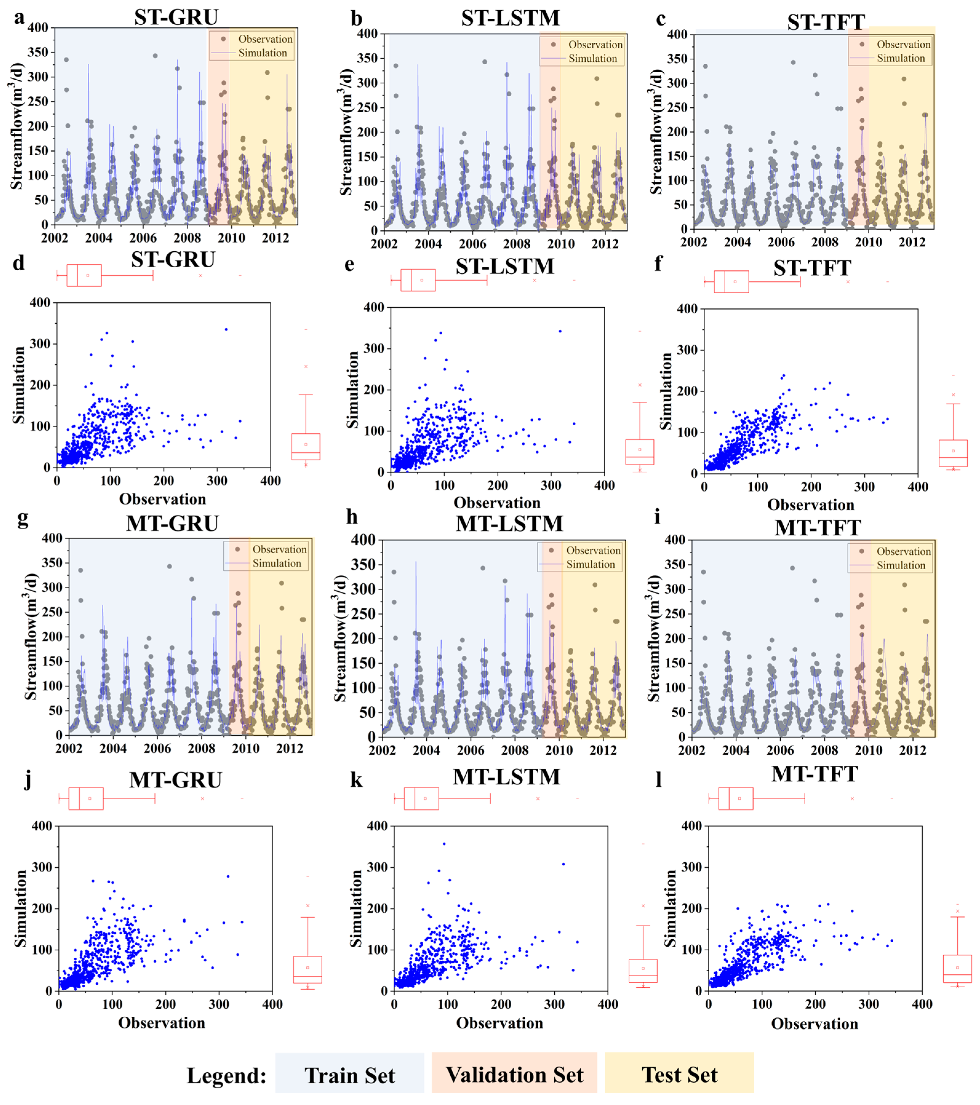
Figure 5 shows the simulated runoff discharge in the middle streams of the HRB for all six models. All models reproduce the periodic runoff variations; however, their skill in capturing peak values varies. As seen in Figure 5d–f,j–l), both GRU- and LSTM-based models consistently underestimate peak flows and slightly overestimate low flows under both STL and MTL frameworks.
By contrast, the Transformer-based TFT exhibits more robust performance in reproducing both peaks and troughs, though peak magnitudes remain slightly underestimated. When comparing frameworks, the MTL approach improves accuracy for all models relative to STL. The MT-TFT achieves the clearest gains, reflecting its capacity to capture complex surface–groundwater interactions in the HRB. Incorporating groundwater-level dynamics as an auxiliary task within the Transformer framework not only enhances surface runoff simulation but also demonstrates potential for representing intricate coupled hydrological processes.

3.2. Cluster Analysis of Groundwater Observation and Analysis of Simulation Results

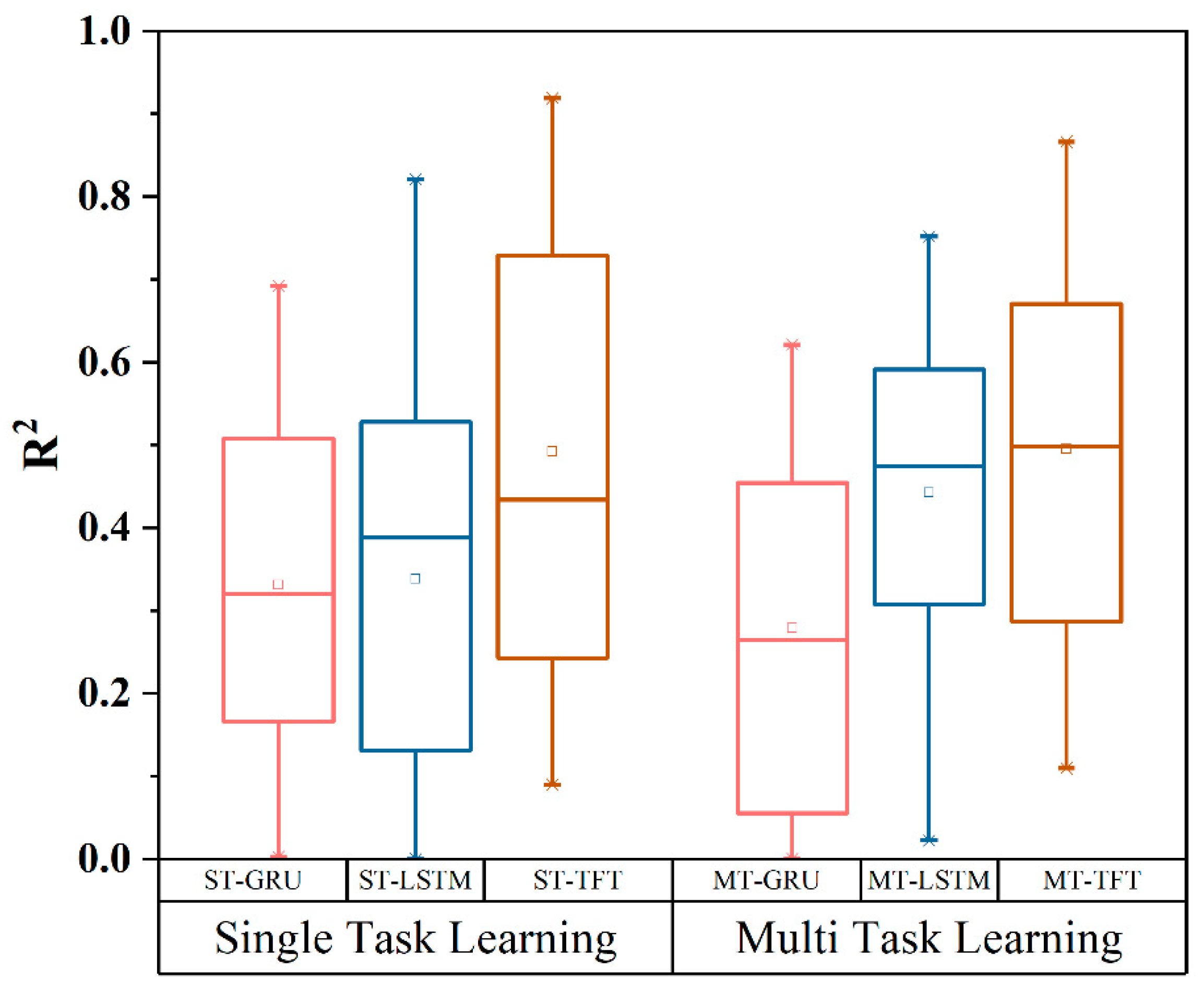
Figure 6 presents the boxplot distributions of the coefficient of determination ( R 2 ) for groundwater-level dynamic simulations at all observation wells in the HRB, obtained from six models under two architectures: single-task learning and multi-task learning. Within the STL framework, the Transformer-based TFT achieved the best performance (median R2 = 0.43; mean R2 = 0.49), outperforming both RNN-based models. The ST-LSTM ranked second (median 0.39; mean 0.33), followed by the ST-GRU (median 0.31; mean 0.32). Despite the ranking, overall accuracy for groundwater simulation under STL was modest, with LSTM showing only a slight edge over GRU.
Under the MTL framework, accuracy improved for TFT and LSTM but declined for GRU. The MT-TFT reached median/mean R2 = 0.52, the MT-LSTM attained 0.49/0.43, and the MT-GRU fell to 0.29/0.30. These results highlight two consistent patterns: TFT consistently outperformed LSTM and GRU in both frameworks, reflecting its architectural advantage, and incorporating surface runoff as an auxiliary task enhanced TFT and LSTM performance, demonstrating MTL’s effectiveness in capturing surface–groundwater interactions in hydrologically complex basins.
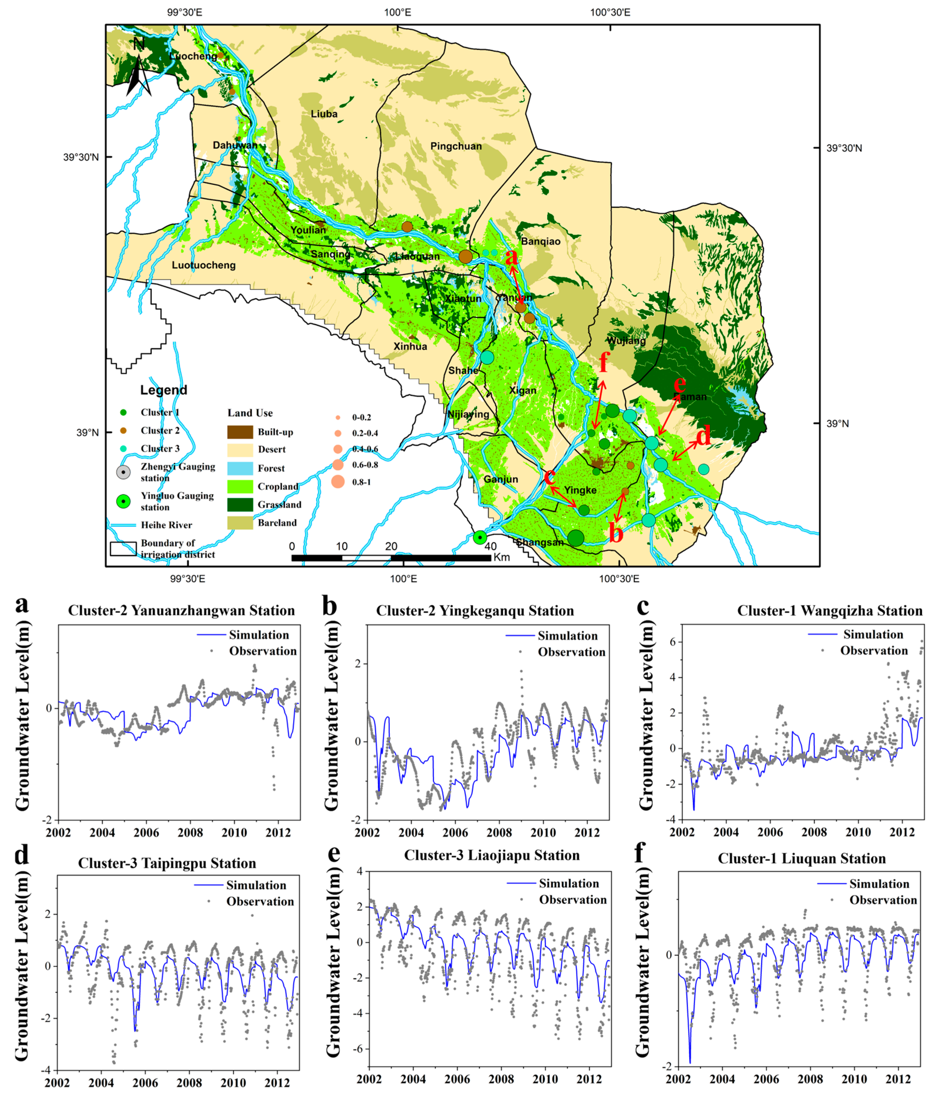
The SOM results (Figure 7) revealed clear spatial heterogeneity, effectively grouping observation stations by proximity to the main channel. Cluster-1 stations (green) are mainly in agricultural areas near the channel, where irrigation and land use strongly affect groundwater; Cluster-2 stations (red) lie along the channel and are influenced by surface water–groundwater interactions; and Cluster-3 stations (blue) are farther away, exhibiting distinctive temporal patterns.
MT-TFT performance varied by cluster (Figure 8a): highest at Cluster-3 stations (median R2 = 0.71; mean = 0.68), intermediate at Cluster-1 stations (median and mean = 0.50), and lowest at Cluster-2 stations (median = 0.45; mean = 0.39). Time-series analyses showed that Cluster-3 stations have greater temporal autocorrelation and more regular seasonal cycles, while Cluster-1 and Cluster-2 stations display higher variability, more complex fluctuations, and frequent outliers.
Permutation Entropy analysis (Figure 8b) confirmed these trends: lowest in Cluster 3 (median = 2.06), moderate in Cluster 2 (2.13), and highest in Cluster 1 (2.19). Permutation Entropy (PE) is a complexity measure for time-series data, based on comparing neighboring values and capturing the order relations between them. The core idea is to analyze the sequence of data points by looking at the ordinal patterns (i.e., the ranking of values) within short segments of the series. The more irregular and unpredictable the time series is, the higher its Permutation Entropy [58]. Higher entropy in clusters closer to the river suggests more complex and variable groundwater conditions, likely driven by land-use change, intricate surface water–groundwater interactions, and human activities such as irrigation and abstraction.
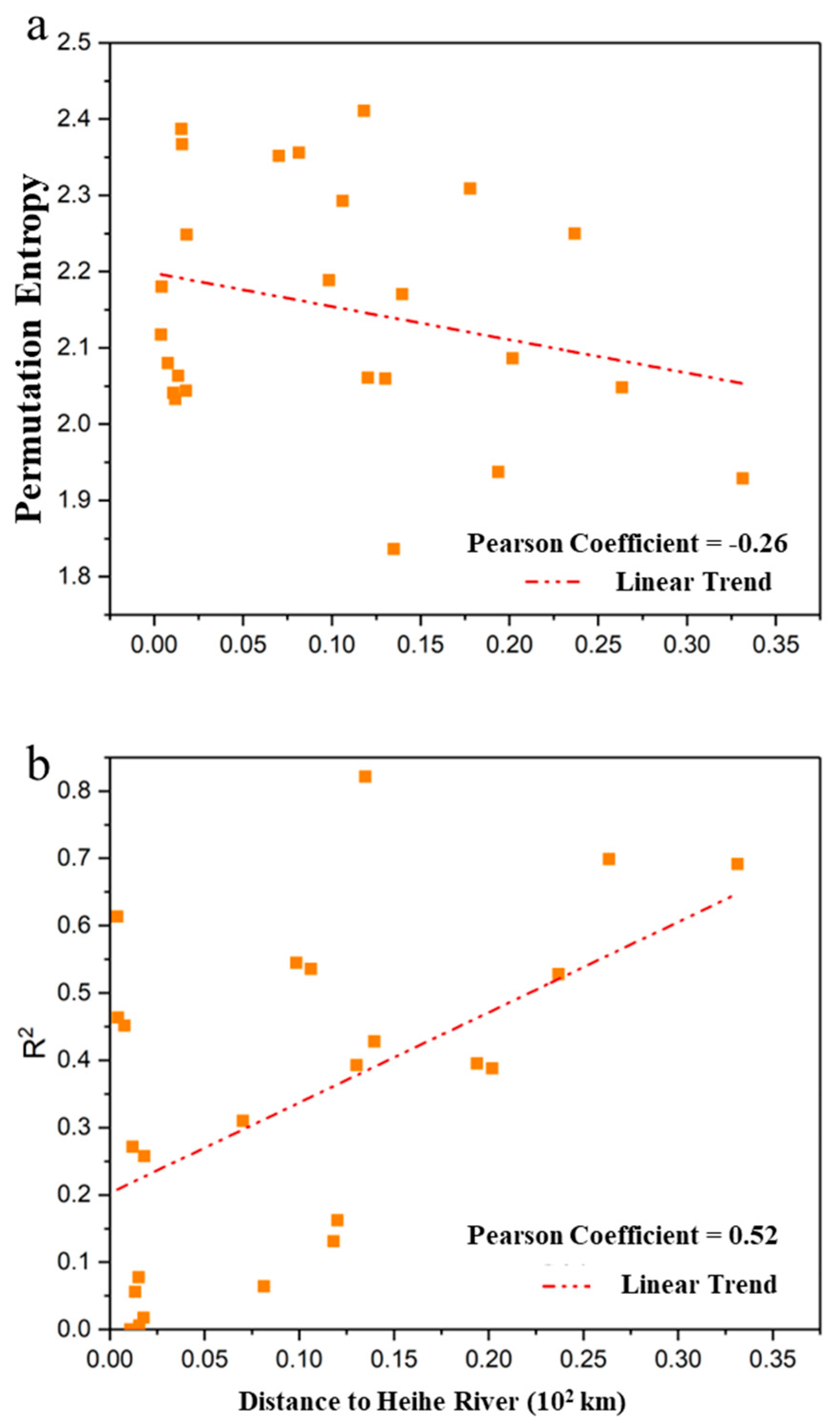
To further investigate the factors influencing the simulation of groundwater-level dynamics, a correlation analysis was performed between the perturbation entropy of groundwater levels, the model’s coefficient of determination (R2) across all monitoring stations, and the geometric distance from each station to the main channel of the HRB (Figure 9). The Pearson correlation coefficient between perturbation entropy and distance to the river was −0.26, indicating a weak negative relationship (Figure 9a). This suggests that stations located closer to the main channel (e.g., Cluster 1 and Cluster 2) tend to have higher perturbation entropy, reflecting greater temporal complexity in groundwater-level dynamics. In contrast, stations farther from the main channel (such as Cluster 3) exhibited lower perturbation entropy, with groundwater dynamics characterized by more regular trends and cyclical variations.
The underlying mechanism for this pattern lies in the role of river proximity in modulating surface water–groundwater interactions. Stations in Cluster 1 and Cluster 2, situated along the Heihe River, experience stronger interactions between groundwater and surface water, resulting in greater variability in groundwater-level fluctuations and, consequently, higher perturbation entropy. In contrast, stations in Cluster 3, located farther from the Heihe River, are less affected by these interactions. In such areas, groundwater dynamics are predominantly influenced by human activities—such as irrigation and pumping—which, particularly in mature irrigated regions, tend to be relatively stable and periodic. This stability contributes to lower perturbation entropy and more pronounced seasonal and trend-related cycles.
Furthermore, the Pearson correlation coefficient between the model’s R2 and the distance from the Heihe River was 0.52, indicating a moderate positive correlation (Figure 9b). This finding implies that the model attains higher simulation accuracy for stations located farther from the river, while performance is comparatively lower at stations nearer to the main channel. The likely reason is that increasing distance reduces the influence of surface water–groundwater interactions, thereby facilitating the model’s ability to capture groundwater-level dynamics. Conversely, near-river stations exhibit more complex and stochastic groundwater patterns, with frequent outliers, which increases simulation difficulty and reduces accuracy.

4. Discussion

4.1. Temporal Analysis of Attention Weights in Runoff Prediction

The Transformer architecture is noted for its powerful attention mechanism, which effectively captures temporal dependencies in spatiotemporal datasets. This section examines how temporal variations in attention weights influence runoff predictions in the HRB.
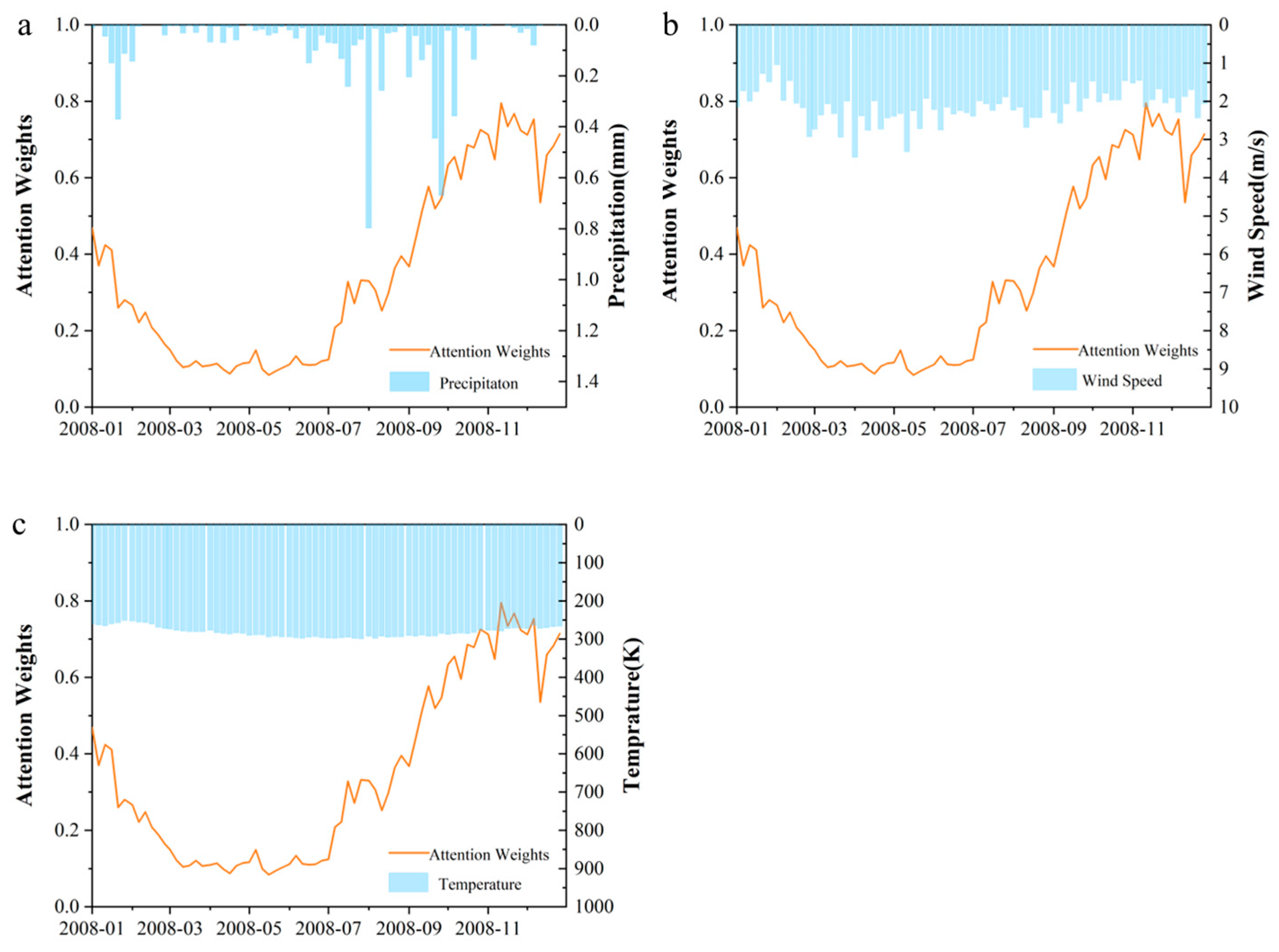
For this analysis, the temporal evolution of attention weights from the multi-task learning MT-TFT model was extracted. The calculation of attention weights can be found in Equation (6). A one-year period preceding the model’s validation phase (2009) was selected, and the evolution of these weights was compared with the corresponding meteorological driving variables—precipitation, air temperature, and wind speed (Figure 10). As shown in Figure 10a, the variation in attention weights closely tracks that of precipitation. In contrast, no consistent patterns were observed between the attention weights and variations in wind speed or air temperature (Figure 10b,c).
Specifically, from January to April, precipitation gradually decreases, and the model’s attention weights decline in parallel. From May to October, increasing precipitation is accompanied by elevated attention weights. As the forecast period approaches (October–December), the weights continue to rise. These fluctuations indicate that the model assigns greater importance to rainfall-related features during periods of high precipitation, effectively identifying and prioritizing predictors most closely associated with runoff generation.
From a hydrological perspective, precipitation is the dominant driver of both rainfall–runoff processes and groundwater recharge in the basin [59,60]. The temporal analysis of attention weights confirms that the MT-TFT model captures this dominant role, concentrating attention on high-precipitation time steps when performing coupled runoff and groundwater forecasts. Toward the end of the forecast horizon, the model further adjusts its weight distribution to enhance the accuracy of near-term, multi-step predictions.

4.2. Factors Influencing the Coupled Surface Water–Groundwater Model

Accurate simulation and prediction of the integrated spatiotemporal dynamics of surface water and groundwater require a detailed examination of the complex relationships between the hydrological processes governing surface runoff and the interactions between surface water and groundwater [61]. This study investigates the factors influencing the performance of the deep learning-based coupled surface water–groundwater spatiotemporal dynamics model by probing the intrinsic relationships among the driving datasets and analyzing the simulation outcomes through an interpretability assessment of the trained model.
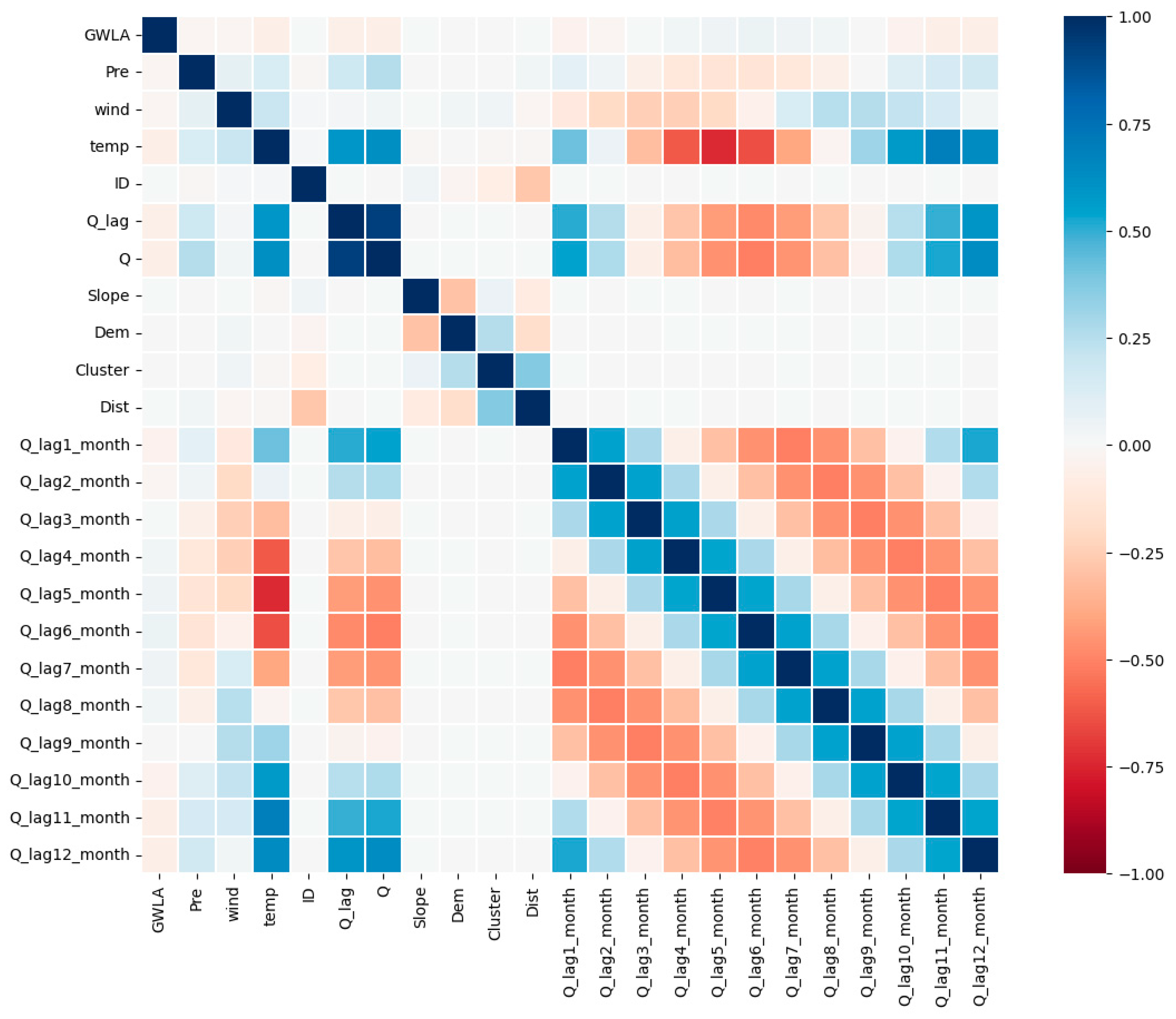
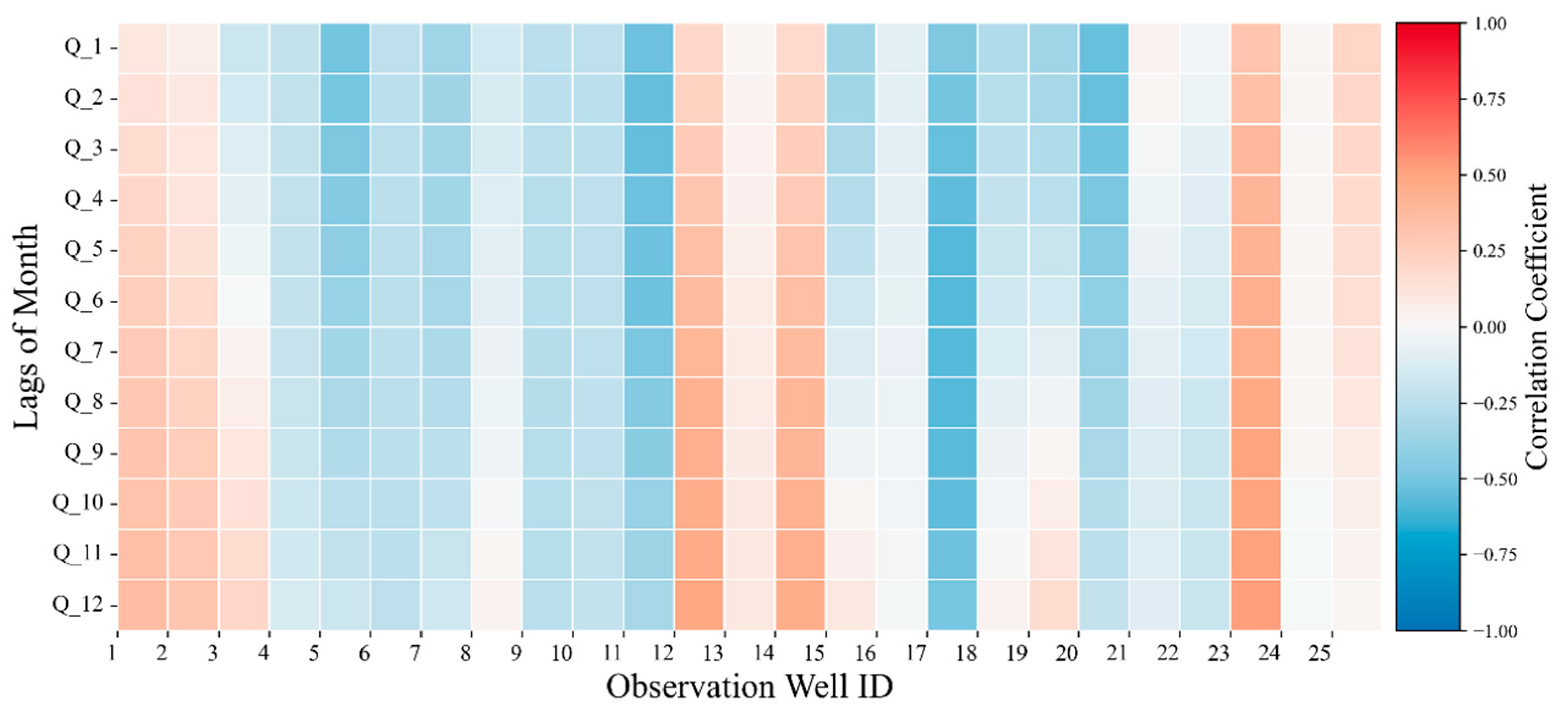
A linear correlation analysis was conducted between all driving variables and the entire set of groundwater observation data (Figure 11). For the groundwater-level time series in the middle streams of the HRB, no strong correlations were found with the full suite of driving variables. However, among all drivers, the correlation with runoff data—both at the current time and for lags of one to twelve months—was relatively higher. Overall, groundwater-level variations in this region were negatively correlated with main-channel runoff, with the strength of correlation varying across lag periods. By contrast, the main-channel runoff time series exhibited significant positive correlations with precipitation and air temperature.
Autocorrelation analysis of the runoff data, using natural months as the time step, revealed a distinct alternating pattern: significant positive correlation, followed by significant negative correlation, and then a return to significant positive correlation across lag periods from one to twelve months (Figure 12). This cyclical behavior reflects the seasonal hydrological regime of the basin and underlines the interconnected nature of runoff and climatic drivers.
In the alluvial plain of the middle streams of the HRB, the groundwater system is closely interconnected with the surface river [62]. Under the combined influences of climate change and irrigation, surface water–groundwater exchanges display pronounced seasonal characteristics. To further examine the relationship between groundwater-level dynamics and runoff from the main channel, a Pearson linear correlation analysis was performed between groundwater observations from all stations and runoff data across lag periods of one to twelve months. As shown in Figure 13, runoff with different lag periods did not exhibit a consistent pattern corresponding to contemporaneous groundwater-level variations at the various observation stations. This result indicates that spatiotemporal variations in groundwater levels in the middle streams of the basin are governed not only by fluctuations in main-channel runoff but also by substantial perturbations from other factors.
Based on the findings in Section 3.2, wells in Cluster 1 (green) are predominantly located in agricultural areas adjacent to the main channel, indicating that land use and human activities (e.g., irrigation) exert a measurable influence on groundwater dynamics. In contrast, wells in Cluster 2 (red) are distributed along the main channel and are primarily affected by surface water–groundwater interaction processes, whereas wells in Cluster 3 (blue) are situated farther from the main channel. In terms of proximity to the HRB, the order is as follows: Cluster-3 wells (furthest) > Cluster-1 wells > Cluster-2 wells (closest).
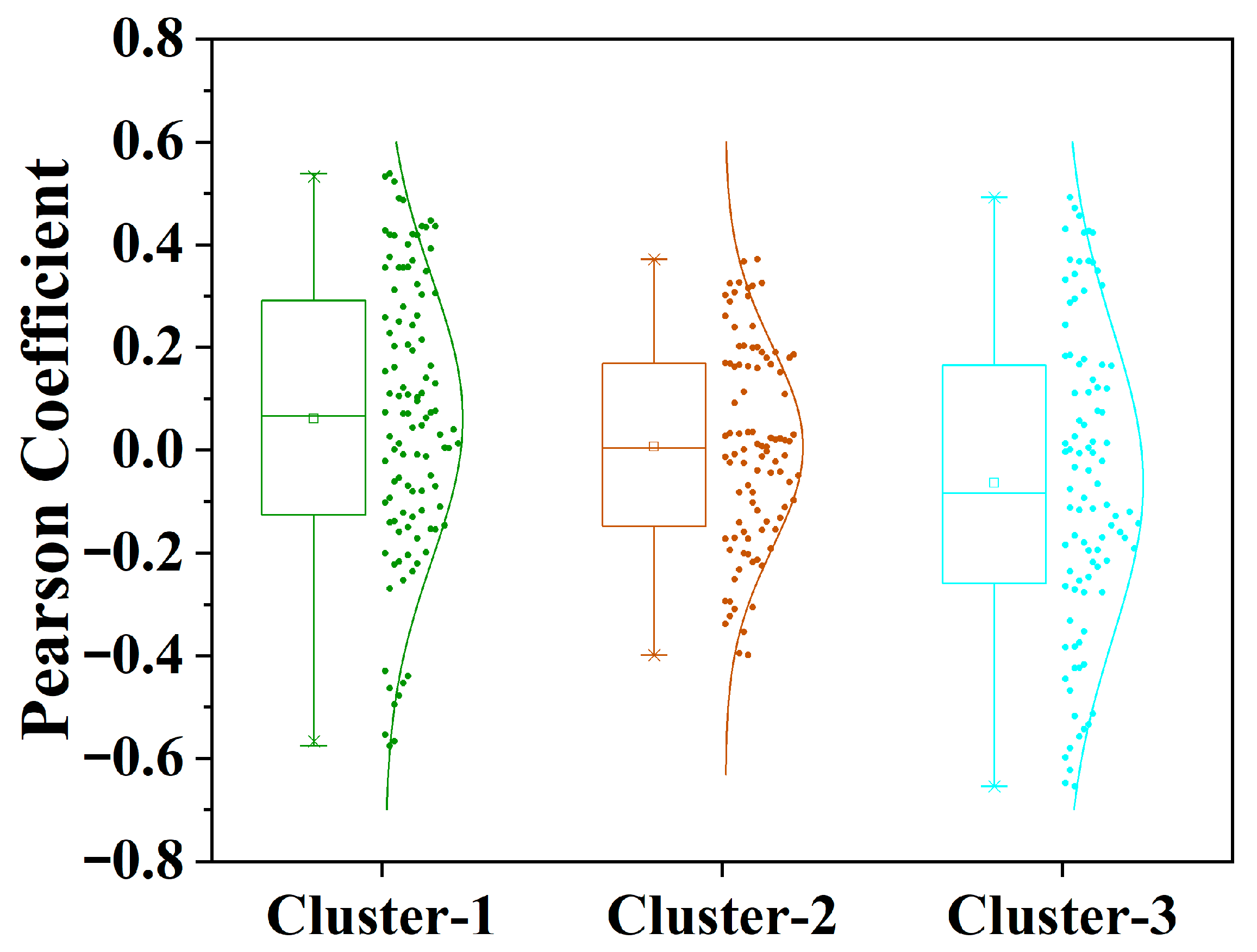
Figure 14 presents the boxplot distributions of the Pearson correlation coefficients between groundwater-level dynamics at all observation wells and the Heihe River runoff at different lag periods (1–12 months), under three SOM clustering results (Cluster 1, Cluster 2, and Cluster 3). As illustrated in Figure 14, the linear correlation between groundwater-level dynamics and surface runoff at different lag periods exhibits distinct patterns across clusters. Cluster 3, farthest from the main channel, shows the highest linear correlation with runoff discharge, followed by Cluster 1, while Cluster 2 displays the lowest correlation. This pattern indicates a negative relationship between the strength of the groundwater–runoff correlation and the proximity of wells to the main channel in the middle streams of the HRB.
Multiple factors contribute to this behavior. The mid-streams of the HRB are characterized by abundant solar and thermal resources, low precipitation, and high evaporation [63]. The creation of artificial oases and a dense canal network has led to extensive diversion of river water for irrigation, reducing downstream discharge [26]. This runoff-utilization zone encompasses key agricultural areas in Gansu Province (e.g., Ganzhou District, Shandan County, Minle County, Linze County, and Gaotai County) as well as parts of Jiuquan (Suzhou District) and Jiayuguan City. In these irrigated oasis basins, groundwater and surface water frequently interact, while climate variability and irrigation practices further influence evapotranspiration. As a result, anthropogenic activities such as irrigation water diversion are both frequent and complex.
Under the combined effects of surface water diversion and groundwater pumping for irrigation, wells in Cluster 2—being closest to the main channel—experience strong, dynamic surface water–groundwater interactions, leading to lower linear correlations between groundwater dynamics and surface runoff. Conversely, Cluster-3 wells, located farther from the main channel, are less affected by these disturbances and thus display higher correlations with runoff data across multiple lag periods.
In the alluvial plain of the middle streams of the HRB, river infiltration and groundwater exfiltration processes are controlled by local hydrogeological conditions, including topography, geology, and land use. As a result, the nature of surface water–groundwater interactions varies among different regional settings. Previous studies by Yao et al. (2015, 2018) [38,39] report that in the mid-to-lower streams of the basin, the magnitude of seasonal variation in surface water–groundwater exchange is substantial. In five river sections within this region, the ratio of groundwater infiltration to river runoff ranges from 5% to 27%. For example, in the Yingluoxia–Heihe 312 Bridge segment—characterized by a deep groundwater table and a thick unsaturated zone—more than 50% of river runoff during the dry season originates from infiltration, compared to only about 10% during the wet season. In contrast, in the mid-streams over the silt plain (Heihe 312 Bridge to Gaoya), groundwater discharge sustains more than 60% of river runoff during the dry season [38,39]. These findings underscore the importance of accurately identifying and quantifying interaction mechanisms and exchange volumes between surface water and groundwater to support the development of robust coupled models.
Given the ability of deep learning algorithms to uncover latent non-linear relationships, an interpretability analysis was conducted on the multi-task learning MT-TFT model based on the Transformer architecture. As shown in Figure 15, the analysis of static input variable importance reveals that the geometric distance from each observation station to the main channel, the SOM-based cluster classification of stations, and the surface slope derived from the digital elevation model (DEM) are the primary influencing factors. For dynamic input variables, runoff data at multiple lag periods receive the highest importance scores—particularly at a monthly resolution for lags of 1, 2, 4, and 11 months. This pattern is consistent with earlier correlation analyses, where the Heihe River’s runoff series exhibited significant positive autocorrelation at lags of 1–4 and 10–12 months (Figure 11 and Figure 12), and groundwater-level dynamics in the mid-streams showed correspondingly high correlations with runoff at lags of 1–3 and 11–12 months. These results highlight the necessity of including runoff lag terms in the simulation framework to capture the delayed aquifer response to meteorological forcing, as well as to account for the effects of water diversion and irrigation practices on surface water–groundwater interactions.

5. Conclusions

This study developed a novel multi-task learning (MTL) framework for coupled surface water–groundwater modeling in the Heihe River Basin (HRB), integrating Transformer architecture with hydrological process analysis. Comprehensive evaluation of model performance and interpretability yielded the following major findings:
(1)
The proposed MTL framework demonstrated significant advantages over single-task learning (STL) approaches in simulating coupled hydrological processes. By jointly optimizing surface runoff and groundwater-level prediction tasks, the MTL framework improved Nash–Sutcliffe efficiency (NSE) and coefficient of determination (R2) by 15–20% across all model configurations using the 2001–2012 HRB datasets.
(2)
The Transformer-based Temporal Fusion Transformer (TFT) algorithm outperformed both GRU and LSTM models in simulating surface runoff and groundwater-level dynamics under both STL and MTL frameworks. Notably, within the MTL setting, the MT-TFT model, which incorporates the groundwater-level simulation task, achieved superior performance in surface runoff prediction (NSE = 0.73; R2 = 0.75), substantially surpassing all STL models.
(3)
Analysis of the model’s attention mechanism revealed that higher attention weights were consistently assigned to time steps with greater precipitation. These weights further increased as the forecast horizon shortened, thereby enhancing the accuracy of near-term multi-step predictions.
(4)
The clustering results of the SOM revealed distinct spatial distribution characteristics and temporal variation patterns in groundwater time-series dynamics among different categories of observation wells. The SOM effectively distinguished observation wells based on their geometric proximity to the Heihe River. Wells located farther away exhibited lower Permutation Entropy in groundwater time-series dynamics, relatively lower temporal complexity, and higher simulation accuracy in the model, and vice versa.
(5)
Pearson linear correlation analysis between groundwater observations and runoff discharge under varying time lags indicates distinct lag-dependent relationships in the mid-stream HRB. Autocorrelation of monthly runoff data showed a cyclical pattern, with correlations shifting from significantly positive to negative and back to positive as lags increased from 1 to 12 months. Spatially, groundwater-level variations exhibited a negative correlation with river discharge in the main stem of the Heihe River, which became more pronounced with increasing geographic distance.

Supplementary Materials

The following supporting information can be downloaded at: https://www.mdpi.com/article/10.3390/hydrology12110291/s1, 1. Brief summary of the LSTM; 2. Brief summary of the GRU.

Author Contributions

H.J.: methodology, writing—original draft, and software. Y.T.: review and editing and supervision. C.Z.: supervision, funding acquisition, review and editing, and project administration. All authors have read and agreed to the published version of the manuscript.

Funding

This work was supported by the National Key R&D Program of China (2023YFC3708001 and 2023YFE0117000) and the National Natural Science Foundation of China (No. 42477053). Additional support was provided by the Guangdong-Hong Kong Joint Laboratory for Soil and Groundwater Pollution Control (No. 2023B1212120001) and the Center for Computational Science and Engineering of Southern University of Science and Technology.

Data Availability Statement

The data that support the findings of this study are available from the corresponding author upon reasonable request. The data are not publicly available due to privacy concerns.

Conflicts of Interest

The authors declare that they have no known competing financial interests or personal relationships that could have appeared to influence the work reported in this paper.

Abbreviations

The following abbreviations are used in this manuscript:
MTLMulti-Task Learning
STLStingle-Task Learning
SW-GWSurface Water–Groundwater
RNNsRecurrent Neural Networks
GRUGated Recurrent Unit
LSTMLong Short-Term Memory
CNNsConvolutional Neural Networks
TFTTemporal Fusion Transformer
GRNGated Residual Network
VSNVariable Selection Network
SCEsStatic Covariate Encoders
TFDTemporal Fusion Decoder
SELStatic Enrichment Layer
TSLTemporal Self-Attention Layer
PFLPosition-wise Feed-forward Layer
ELUExponential Linear Unit
GLUsGated Linear Units
RMSERoot Mean Square Error
NSENash–Sutcliffe Efficiency
R2Coefficient of Determination
HRBHeihe River Basin
IoTInternet of Things
PRMSsPrecipitation–Runoff Modeling Systems
SOMSelf-Organizing Map

References

  1. Aeschbach-Hertig, W.; Gleeson, T. Regional strategies for the accelerating global problem of groundwater depletion. Nat. Geosci. 2012, 5, 853–861. [Google Scholar] [CrossRef]
  2. Kuang, X.; Liu, J.; Scanlon, B.R.; Jiao, J.J.; Jasechko, S.; Lancia, M.; Biskaborn, B.K.; Wada, Y.; Li, H.; Zeng, Z.; et al. The changing nature of groundwater in the global water cycle. Science 2024, 383, eadf0630. [Google Scholar] [CrossRef] [PubMed]
  3. Scanlon, B.R.; Jolly, I.; Sophocleous, M.; Zhang, L. Global impacts of conversions from natural to agricultural ecosystems on water resources: Quantity versus quality. Water Resour. Res. 2007, 43, W03437. [Google Scholar] [CrossRef]
  4. Siebert, S.; Burke, J.; Faures, J.M.; Frenken, K.; Hoogeveen, J.; Döll, P.; Portmann, F.T. Groundwater use for irrigation–a global inventory. Hydrol. Earth Syst. Sci. 2010, 14, 1863–1880. [Google Scholar] [CrossRef]
  5. Scanlon, B.R.; Fakhreddine, S.; Rateb, A.; de Graaf, I.; Famiglietti, J.; Gleeson, T.; Grafton, R.Q.; Jobbagy, E.; Kebede, S.; Kolusu, S.R.; et al. Global water resources and the role of groundwater in a resilient water future. Nat. Rev. Earth Environ. 2023, 4, 87–101. [Google Scholar] [CrossRef]
  6. Döll, P.; Hoffmann-Dobrev, H.; Portmann, F.T.; Siebert, S.; Eicker, A.; Rodell, M.; Strassberg, G.; Scanlon, B.R. Impact of water withdrawals from groundwater and surface water on continental water storage variations. J. Geodyn. 2012, 59–60, 143–156. [Google Scholar] [CrossRef]
  7. Lancia, M.; Yao, Y.; Andrews, C.B.; Wang, X.; Kuang, X.; Ni, J.; Gorelick, S.M.; Scanlon, B.R.; Wang, Y.; Zheng, C. The China groundwater crisis: A mechanistic analysis with implications for global sustainability. Sustain. Horiz. 2022, 4, 100042. [Google Scholar] [CrossRef]
  8. Gorelick, S.M.; Zheng, C. Global change and the groundwater management challenge. Water Resour. Res. 2015, 51, 3031–3051. [Google Scholar] [CrossRef]
  9. Sophocleous, M. From safe yield to sustainable development of water resources—The Kansas experience. J. Hydrol. 2000, 235, 27–43. [Google Scholar] [CrossRef]
  10. Kendy, E.; Gérard-Marchant, P.; Todd Walter, M.; Zhang, Y.; Liu, C.; Steenhuis, T.S. A soil-water-balance approach to quantify groundwater recharge from irrigated cropland in the North China Plain. Hydrol. Process. 2003, 17, 2011–2031. [Google Scholar] [CrossRef]
  11. Kinzelbach, W.; Bauer, P.; Siegfried, T.; Brunner, P. Sustainable groundwater management--Problems and scientific tool. Epis. -Newsmag. Int. Union Geol. Sci. 2003, 26, 279–284. [Google Scholar] [CrossRef]
  12. He, Q.; Liu, W.; Li, Z. Land Subsidence Survey and Monitoringin the North China Plain. Geol. J. China Univ. 2006, 12, 195–209. [Google Scholar]
  13. Aderemi, B.A.; Olwal, T.O.; Ndambuki, J.M.; Rwanga, S.S. A Review of Groundwater Management Models with a Focus on IoT-Based Systems. Sustainability 2022, 14, 148. [Google Scholar] [CrossRef]
  14. Shen, C. A Transdisciplinary Review of Deep Learning Research and Its Relevance for Water Resources Scientists. Water Resour. Res. 2018, 54, 8558–8593. [Google Scholar] [CrossRef]
  15. Zhang, J.; Zhu, Y.; Zhang, X.; Ye, M.; Yang, J. Developing a Long Short-Term Memory (LSTM) based model for predicting water table depth in agricultural areas. J. Hydrol. 2018, 561, 918–929. [Google Scholar] [CrossRef]
  16. Rajaee, T.; Ebrahimi, H.; Nourani, V. A review of the artificial intelligence methods in groundwater level modeling. J. Hydrol. 2019, 572, 336–351. [Google Scholar] [CrossRef]
  17. Chen, C.; He, W.; Zhou, H.; Xue, Y.; Zhu, M. A comparative study among machine learning and numerical models for simulating groundwater dynamics in the Heihe River Basin, northwestern China. Sci. Rep. 2020, 10, 3904. [Google Scholar] [CrossRef]
  18. Xiang, Z.; Yan, J.; Demir, I. A Rainfall-Runoff Model With LSTM-Based Sequence-to-Sequence Learning. Water Resour. Res. 2020, 56, e2019WR025326. [Google Scholar] [CrossRef]
  19. Sun, J.; Hu, L.; Li, D.; Sun, K.; Yang, Z. Data-driven models for accurate groundwater level prediction and their practical significance in groundwater management. J. Hydrol. 2022, 608, 127630. [Google Scholar] [CrossRef]
  20. Tian, W.; Li, X.; Cheng, G.D.; Wang, X.S.; Hu, B.X. Coupling a groundwater model with a land surface model to improve water and energy cycle simulation. Hydrol. Earth Syst. Sci. 2012, 16, 4707–4723. [Google Scholar] [CrossRef]
  21. Kratzert, F.; Klotz, D.; Brenner, C.; Schulz, K.; Herrnegger, M. Rainfall–runoff modelling using Long Short-Term Memory (LSTM) networks. Hydrol. Earth Syst. Sci. 2018, 22, 6005–6022. [Google Scholar] [CrossRef]
  22. Kratzert, F.; Klotz, D.; Herrnegger, M.; Sampson, A.K.; Hochreiter, S.; Nearing, G.S. Toward Improved Predictions in Ungauged Basins: Exploiting the Power of Machine Learning. Water Resour. Res. 2019, 55, 11344–11354. [Google Scholar] [CrossRef]
  23. Kratzert, F.; Klotz, D.; Shalev, G.; Klambauer, G.; Hochreiter, S.; Nearing, G. Towards learning universal, regional, and local hydrological behaviors via machine learning applied to large-sample datasets. Hydrol. Earth Syst. Sci. 2019, 23, 5089–5110. [Google Scholar] [CrossRef]
  24. Ma, K.; Feng, D.; Lawson, K.; Tsai, W.P.; Liang, C.; Huang, X.; Sharma, A.; Shen, C. Transferring Hydrologic Data Across Continents–Leveraging Data-Rich Regions to Improve Hydrologic Prediction in Data-Sparse Regions. Water Resour. Res. 2021, 57, e2020WR028600. [Google Scholar] [CrossRef]
  25. Jiang, S.; Zheng, Y.; Babovic, V.; Tian, Y.; Han, F. A computer vision-based approach to fusing spatiotemporal data for hydrological modeling. J. Hydrol. 2018, 567, 25–40. [Google Scholar] [CrossRef]
  26. Li, X.; Cheng, G.; Ge, Y.; Li, H.; Han, F.; Hu, X.; Tian, W.; Tian, Y.; Pan, X.; Nian, Y.; et al. Hydrological Cycle in the Heihe River Basin and Its Implication for Water Resource Management in Endorheic Basins. J. Geophys. Res. Atmos. 2018, 123, 890–914. [Google Scholar] [CrossRef]
  27. Jing, H.; He, X.; Tian, Y.; Lancia, M.; Cao, G.; Crivellari, A.; Guo, Z.; Zheng, C. Comparison and interpretation of data-driven models for simulating site-specific human-impacted groundwater dynamics in the North China Plain. J. Hydrol. 2023, 616, 128751. [Google Scholar] [CrossRef]
  28. Wen, X.H.; Wu, Y.Q.; Lee, L.J.E.; Su, J.P.; Wu, J. Groundwater flow modeling in the Zhangye Basin, Northwestern China. Environ. Geol. 2007, 53, 77–84. [Google Scholar] [CrossRef]
  29. Mi, L.; Xiao, H.; Zhang, J.; Yin, Z.; Shen, Y. Evolution of the groundwater system under the impacts of human activities in middle reaches of Heihe River Basin (Northwest China) from 1985 to 2013. Hydrogeol. J. 2016, 24, 971–986. [Google Scholar] [CrossRef]
  30. Yao, Y.; Zheng, C.; Tian, Y.; Liu, J.; Zheng, Y. Numerical modeling of regional groundwater flow in the Heihe River Basin, China: Advances and new insights. Sci. China Earth Sci. 2015, 58, 3–15. [Google Scholar] [CrossRef]
  31. Jiang, X.-W.; Wan, L.; Wang, X.-S.; Ge, S.; Liu, J. Effect of exponential decay in hydraulic conductivity with depth on regional groundwater flow. Geophys. Res. Lett. 2009, 36, L24402. [Google Scholar] [CrossRef]
  32. Miguez-Macho, G.; Fan, Y. The role of groundwater in the Amazon water cycle: 2. Influence on seasonal soil moisture and evapotranspiration. J. Geophys. Res. Atmos. 2012, 117, D15114. [Google Scholar] [CrossRef]
  33. Pokhrel, Y.N.; Fan, Y.; Miguez-Macho, G.; Yeh, P.J.-F.; Han, S.-C. The role of groundwater in the Amazon water cycle: 3. Influence on terrestrial water storage computations and comparison with GRACE. J. Geophys. Res. Atmos. 2013, 118, 3233–3244. [Google Scholar] [CrossRef]
  34. Kuang, X.; Jiao, J.J. An integrated permeability-depth model for Earth’s crust. Geophys. Res. Lett. 2014, 41, 7539–7545. [Google Scholar] [CrossRef]
  35. Yang, K.; He, J.; Tang, W.; Lu, H.; Qin, J.; Chen, Y.; Li, X. China Meteorological Forcing Dataset V1.6 (1979–2018). National Tibetan Plateau / Third Pole Environment Data Center. 2019. Available online: https://data.tpdc.ac.cn/en/data/8028b944-daaa-4511-8769-965612652c49 (accessed on 29 October 2025).
  36. He, J.; Yang, K.; Tang, W.; Lu, H.; Qin, J.; Chen, Y.; Li, X. The first high-resolution meteorological forcing dataset for land process studies over China. Sci. Data 2020, 7, 25. [Google Scholar] [CrossRef]
  37. Yang, K.; He, J.; Tang, W.; Qin, J.; Cheng, C.C.K. On downward shortwave and longwave radiations over high altitude regions: Observation and modeling in the Tibetan Plateau. Agric. For. Meteorol. 2010, 150, 38–46. [Google Scholar] [CrossRef]
  38. Yao, Y.; Huang, X.; Liu, J.; Zheng, C.; He, X.; Liu, C. Spatiotemporal variation of river temperature as a predictor of groundwater/surface-water interactions in an arid watershed in China. Hydrogeol. J. 2015, 23, 999–1007. [Google Scholar] [CrossRef]
  39. Yao, Y.; Zheng, C.; Tian, Y.; Li, X.; Liu, J. Eco-hydrological effects associated with environmental flow management: A case study from the arid desert region of China. Ecohydrology 2018, 11, e1914. [Google Scholar] [CrossRef]
  40. Crawshaw, M. Multi-task learning with deep neural networks: A survey. arXiv 2020, arXiv:2009.09796. [Google Scholar] [CrossRef]
  41. Caruana, R. Multitask learning. Mach. Learn. 1997, 28, 41–75. [Google Scholar] [CrossRef]
  42. Medsker, L.R.; Jain, L. Recurrent neural networks. Des. Appl. 2001, 5, 2. [Google Scholar]
  43. Hochreiter, S.; Schmidhuber, J. Long short-term memory. Neural Comput. 1997, 9, 1735–1780. [Google Scholar] [CrossRef]
  44. Cho, K.; van Merriënboer, B.; Bahdanau, D.; Bengio, Y. On the Properties of Neural Machine Translation: Encoder–Decoder Approaches. Association for Computational Linguistics. 2014, pp. 103–111. Available online: https://aclanthology.org/W14-4012/ (accessed on 29 October 2025).
  45. Mienye, I.D.; Swart, T.G. A Comprehensive Review of Deep Learning: Architectures, Recent Advances, and Applications. Information 2024, 15, 755. [Google Scholar] [CrossRef]
  46. LeCun, Y.; Bengio, Y.; Hinton, G. Deep learning. Nature 2015, 521, 436–444. [Google Scholar] [CrossRef] [PubMed]
  47. Lim, B.; Arık, S.Ö.; Loeff, N.; Pfister, T. Temporal Fusion Transformers for interpretable multi-horizon time series forecasting. Int. J. Forecast. 2021, 37, 1748–1764. [Google Scholar] [CrossRef]
  48. Rasiya Koya, S.; Roy, T. Temporal Fusion Transformers for streamflow Prediction: Value of combining attention with recurrence. J. Hydrol. 2024, 637, 131301. [Google Scholar] [CrossRef]
  49. Fayer, G.; Lima, L.; Miranda, F.; Santos, J.; Campos, R.; Bignoto, V.; Andrade, M.; Moraes, M.; Ribeiro, C.; Capriles, P.; et al. A Temporal Fusion Transformer Deep Learning Model for Long-Term Streamflow Forecasting: A Case Study in the Funil Reservoir, Southeast Brazil. Knowl.-Based Eng. Sci. 2023, 4, 73–88. [Google Scholar]
  50. Francisco, R.; Matos, J.P.; Marinheiro, R.; Lopes, N.; Portela, M.M.; Barros, P. Application of Temporal Fusion Transformers to Run-Of-The-River Hydropower Scheduling. Hydrology 2025, 12, 81. [Google Scholar] [CrossRef]
  51. Zhou, R.; Wang, Q.; Jin, A.; Shi, W.; Liu, S. Interpretable multi-step hybrid deep learning model for karst spring discharge prediction: Integrating temporal fusion transformers with ensemble empirical mode decomposition. J. Hydrol. 2024, 645, 132235. [Google Scholar] [CrossRef]
  52. Jiang, M.; Weng, B.; Chen, J.; Huang, T.; Ye, F.; You, L. Transformer-enhanced spatiotemporal neural network for post-processing of precipitation forecasts. J. Hydrol. 2024, 630, 130720. [Google Scholar] [CrossRef]
  53. Kohonen, T. Self-organized formation of topologically correct feature maps. Biol. Cybern. 1982, 43, 59–69. [Google Scholar] [CrossRef]
  54. Probst, P.; Wright, M.N.; Boulesteix, A.-L. Hyperparameters and tuning strategies for random forest. WIREs Data Min. Knowl. Discov. 2019, 9, e1301. [Google Scholar] [CrossRef]
  55. O’Malley, T.; Bursztein, E.; Long, J.; Chollet, F.; Jin, H.; Invernizzi, L. KerasTuner. 2019. Available online: https://github.com/keras-team/keras-tuner (accessed on 2 March 2021).
  56. Onyutha, C. A hydrological model skill score and revised R-squared. Hydrol. Res. 2021, 53, 51–64. [Google Scholar] [CrossRef]
  57. Krause, P.; Boyle, D.P.; Bäse, F. Comparison of different efficiency criteria for hydrological model assessment. Adv. Geosci. 2005, 5, 89–97. [Google Scholar] [CrossRef]
  58. Bandt, C.; Pompe, B. Permutation Entropy: A Natural Complexity Measure for Time Series. Phys. Rev. Lett. 2002, 88, 174102. [Google Scholar] [CrossRef]
  59. Feng, Z.; Liu, S.; Guo, Y.; Liu, X. Runoff Responses of Various Driving Factors in a Typical Basin in Beijing-Tianjin-Hebei Area. Remote Sens. 2023, 15, 1027. [Google Scholar] [CrossRef]
  60. Wittenberg, H.; Aksoy, H.; Miegel, K. Fast response of groundwater to heavy rainfall. J. Hydrol. 2019, 571, 837–842. [Google Scholar] [CrossRef]
  61. Ntona, M.M.; Busico, G.; Mastrocicco, M.; Kazakis, N. Modeling groundwater and surface water interaction: An overview of current status and future challenges. Sci. Total Environ. 2022, 846, 157355. [Google Scholar] [CrossRef] [PubMed]
  62. Yao, Y.; Tian, Y.; Andrews, C.; Li, X.; Zheng, Y.; Zheng, C. Role of Groundwater in the Dryland Ecohydrological System: A Case Study of the Heihe River Basin. J. Geophys. Res. Atmos. 2018, 123, 6760–6776. [Google Scholar] [CrossRef]
  63. Wu, H.; Xue, H.; Dong, G.; Gao, J.; Lian, Y.; Li, Z. Runoff variation in midstream Hei River, northwest China: Characteristics and driving factors analysis. J. Hydrol. Reg. Stud. 2024, 53, 101764. [Google Scholar] [CrossRef]
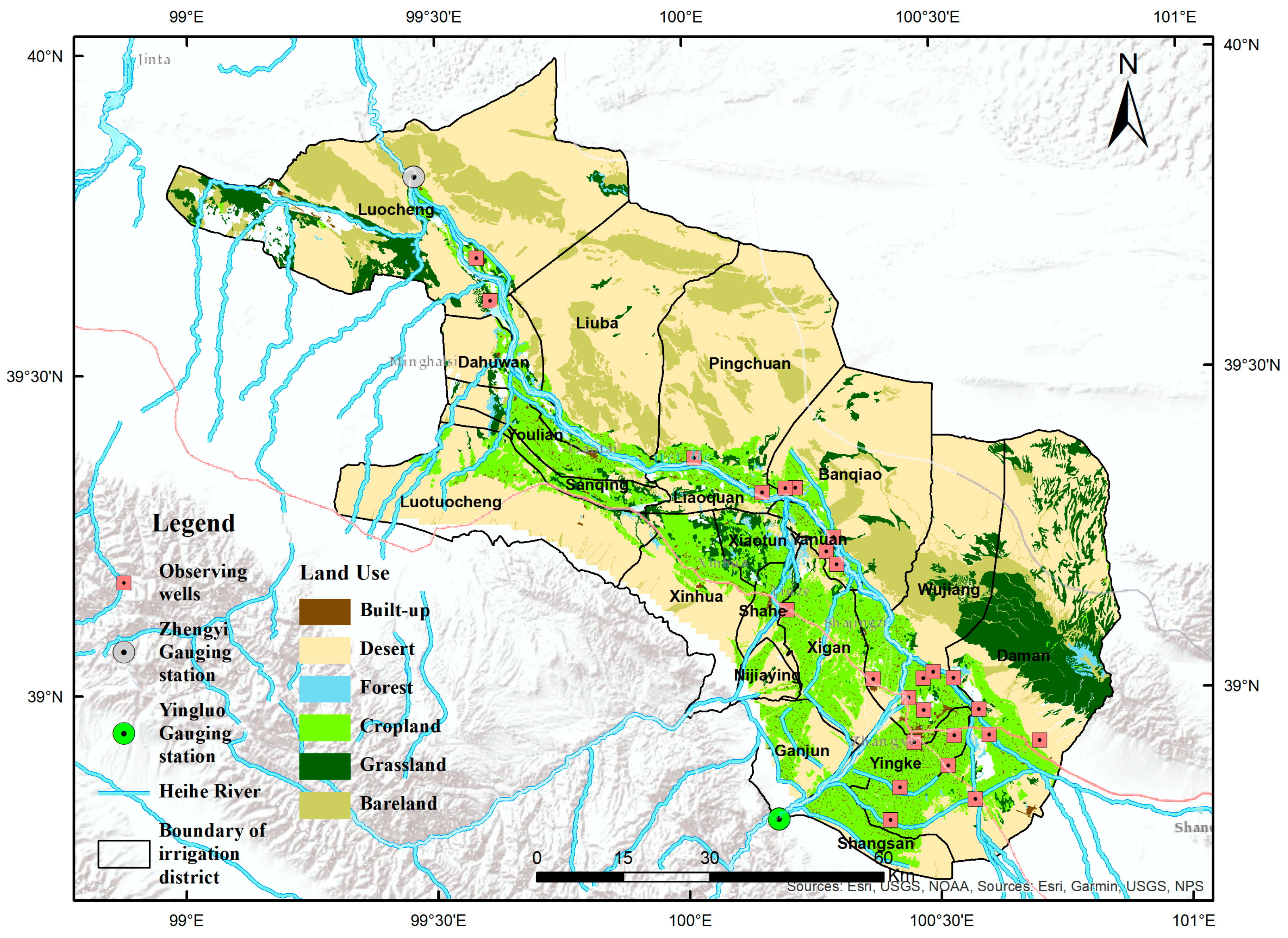
Figure 1. Location of the Heihe River Basin (HRB) and groundwater observation wells.
Hydrology 12 00291 g001
Figure 2. Conceptual model of surface water and groundwater coupling process in HRB.
Hydrology 12 00291 g002
Figure 3. Multi-task learning framework based on LSTM and GRU, designed for simulating coupled surface water–groundwater processes.
Hydrology 12 00291 g003
Figure 4. Multi-task learning framework based on TFT [47].
Hydrology 12 00291 g004
Figure 5. Six proposed models’ simulation results for runoff in HRB: Streamflow simulation results of (a) ST-GRU, (b) ST-LSTM, (c) ST-TFT, (g) MT-GRU, (h) MT-LSTM, and (i) MT-TFT; Scatter plot of observation and simulation results of (d) ST-GRU, (e) ST-LSTM, (f) ST-TFT, (j) MT-GRU, (k) MT-LSTM, (l) MT-TFT. TFT achieved the best overall performance in both STL and MTL.
Hydrology 12 00291 g005
Figure 6. Box–whisker plot of R2 for groundwater models.
Hydrology 12 00291 g006
Figure 7. Observation clustering results based on SOM and groundwater-level simulation results on selected wells: (a) Cluster-2 Yanuanzhangwan Station, (b) Cluster-2 Yingkeganqu Station, (c) Cluster-1 Wangqizha Station, (d) Cluster-3 Taipingpu Station, (e) Cluster-3 Liaojiapu Station and (f) Cluster-1 Liuquan Station, (different colors and sizes lead to different cluster results and R2 values).
Hydrology 12 00291 g007
Figure 8. Box–whisker plot of (a) R2 and (b) Permutation Entropy of MT-TFT at different observation clusters.
Hydrology 12 00291 g008
Figure 9. Relationship of the distance to HRB with the groundwater modeling performance: (a) Permutation Entropy and (b) R2.
Hydrology 12 00291 g009
Figure 10. Mismatch of the attention on time step: (a) precipitation, (b) wind speed, and (c) temperature.
Hydrology 12 00291 g010
Figure 11. Pearson correlation coefficient between groundwater levels and driving factors.
Hydrology 12 00291 g011
Figure 12. Autocorrelation of runoff in HRB.
Hydrology 12 00291 g012
Figure 13. Heatmap of Pearson correlation relationships between runoff flow and groundwater dynamic data at different lag periods.
Hydrology 12 00291 g013
Figure 14. Boxplot of Pearson correlation coefficient between runoff and groundwater-level data at different lag periods under clustering results of different observation stations.
Hydrology 12 00291 g014
Figure 15. Explanatory results of MT-TFT: (a) static features; (b) encoder features.
Hydrology 12 00291 g015
Table 1. Dataset summary, including source and resolution.
DatasetSourceVariablesSpatial
Resolution
Temporal
Resolution
Meteorological Driving ForceChina Meteorological Forcing DatasetWind0.1°Hourly
Precipitation0.1°Hourly
Temperature0.1°Hourly
GWLWater Resources Department of Gansu ProvinceGroundwater levelIn situ5 Days
StreamflowStreamflowIn situDaily
Land UseSentinel-2LULC30 mYearly
Table 2. Experiment design for model comparison.
Model ArchitectureModel AlgorithmSimulation Target
Single-Task LearningST-GRUSurface Runoff
ST-LSTM
ST-TFT
ST-GRUGroundwater Dynamics
ST-LSTM
ST-TFT
Multi-Task LearningMT-GRUSurface Runoff and Groundwater Dynamics
MT-LSTM
MT-TFT
Table 3. Simulated result metrics of six surface runoff models.
ModelNSER2RMSE (m3/d)
ST-GRU0.510.5239.53
MT-GRU0.450.4941.69
ST-LSTM0.400.4245.66
MT-LSTM0.480.4940.38
ST-TFT0.660.6828.76
MT-TFT0.730.7528.43
Disclaimer/Publisher’s Note: The statements, opinions and data contained in all publications are solely those of the individual author(s) and contributor(s) and not of MDPI and/or the editor(s). MDPI and/or the editor(s) disclaim responsibility for any injury to people or property resulting from any ideas, methods, instructions or products referred to in the content.