Improved Streamflow Forecasting Through SWE-Augmented Spatio-Temporal Graph Neural Networks

Abstract

Streamflow forecasting in snowmelt-dominated basins is essential for water resource planning, flood mitigation, and ecological sustainability. This study presents a comparative evaluation of statistical, machine learning (Random Forest), and deep learning models (Long Short-Term Memory (LSTM), Gated Recurrent Unit (GRU), and Spatio-Temporal Graph Neural Network (STGNN)) using 30 years of data from 20 monitoring stations across the Upper Colorado River Basin (UCRB). We assess the impact of integrating meteorological variables—particularly, the Snow Water Equivalent (SWE)—and spatial dependencies on predictive performance. Among all models, the Spatio-Temporal Graph Neural Network (STGNN) achieved the highest accuracy, with a Nash–Sutcliffe Efficiency (NSE) of 0.84 and Kling–Gupta Efficiency (KGE) of 0.84 in the multivariate setting at the critical downstream node, Lees Ferry. Compared to the univariate setup, SWE-enhanced predictions reduced Root Mean Square Error (RMSE) by 12.8%. Seasonal and spatial analyses showed the greatest improvements at high-elevation and mid-network stations, where snowmelt dynamics dominate runoff. These findings demonstrate that spatio-temporal learning frameworks, especially STGNNs, provide a scalable and physically consistent approach to streamflow forecasting under variable climatic conditions.

1. Introduction

Accurate prediction of streamflow in basins driven by snowmelt is essential for the sustainable management of water resources, mitigation of flood risks, operation of hydropower facilities, and maintenance of ecological resilience [1,2]. In regions characterized by mountainous terrain and high latitudes, snowmelt serves as the primary determinant of seasonal streamflow variability, significantly influencing downstream water supply and ecosystem services [3]. Streamflow forecasts are increasingly important under changing climate regimes, providing the basis for the allocation of water for agricultural, municipal, and industrial use [4] while also supporting early warning systems for extreme events [5]. However, predicting streamflow in such regions is challenged by the nonstationary and spatially complex dynamics of snowpack accumulation and melt [6], especially as warming temperatures intensify variability in hydrological response [7].

Early advances in streamflow prediction were driven by conceptual hydrological models such as the Soil Moisture Accounting model, the HBV (Hydrologiska Byråns Vattenbalansavdelning) model, and the Sacramento model [8,9]. These models introduced foundational principles of watershed-scale water balance, employing lumped or semi-distributed approaches to simulate runoff generation. While impactful, the reliance on extensive site-specific calibration and oversimplified spatial representations limited their predictive accuracy in snow-influenced basins characterized by complex topography and highly variable snowpack. Such models often struggle to represent snowmelt-driven processes that are inherently nonlinear and spatially variable [10].

To better represent snowpack processes, dedicated snowmelt runoff models emerged, such as the Snowmelt Runoff Model (SRM) using temperature-index methods [11]. Physically based models like SNOW-17 [12] further improved realism by simulating snow accumulation, metamorphism, and melt. However, limitations in spatial resolution and dependence on sparse in situ snow observations continued to hinder their widespread application and forecast accuracy [13].

The advent of remote sensing revolutionized snow hydrology by providing gridded and temporally continuous data on snow cover and the snow water equivalent (SWE) across remote terrain [14,15]. Satellite-derived SWE products such as those from AMSR-E, MODIS, and NASA’s SnowEx missions have significantly enhanced hydrological model initialization and updating, particularly to improve spring runoff forecasts in snow-dominated watersheds [16,17].

A paradigm shift occurred with the integration of machine learning (ML) techniques, which excel at learning nonlinear patterns from large, heterogeneous datasets [18,19,20,21,22]. Approaches such as Artificial Neural Networks (ANNs), Support Vector Regression (SVR), Random Forests (RFs), and hybrid ensemble models have been successfully applied in streamflow prediction tasks [23,24]. ML models have also been used to correct biases in physics-based forecasts and improve generalization across basins [25].

Deep learning (DL) architectures such as Long Short-Term Memory (LSTM) networks have further advanced temporal modeling by capturing long-range dependencies in hydrological time series [26,27,28]. LSTM models, along with convolutional neural networks (CNNs), have shown superior performance in handling the memory and dynamics of snow-influenced hydrological systems compared to both traditional and ML approaches [29,30].

While DL models model temporal dynamics effectively, they often neglect explicit spatial dependencies. Spatio-Temporal Graph Neural Networks (STGNNs) overcome this by encoding both spatial and temporal relationships [31]. In hydrology, this means treating gauging stations as graph nodes and connecting them based on hydrological flow paths, allowing upstream information to be propagated and learned within the network [32]. STGNNs have been shown to outperform site-based DL models by leveraging spatial dependencies across multiple basins [33].

The SWE is a key determinant of melt-season streamflow peaks in snow-dominated watersheds [34]. Its inclusion in forecasting models has consistently improved predictive accuracy, especially during spring and early summer [35]. Recent studies have made valuable progress toward improved streamflow prediction. Ensemble-based machine learning approaches have enhanced monthly runoff forecasts by leveraging complementary model strengths [36]. Similarly, spatio-temporal deep learning frameworks with multi-dimensional hidden structures have demonstrated the ability to capture complex flood dynamics [37]. These works underscore the importance of advanced fusion strategies and spatial–temporal representations in hydrological prediction.

Despite advances in deep learning and graph-based modeling, systematic integration of the SWE—particularly from remote sensing—into STGNN frameworks remains limited. Several challenges contribute to this gap. First, remote sensing SWE products often carry significant uncertainties in complex terrain, especially under forest canopies and steep slopes, and frequently require downscaling before use [6,34]. Second, aligning SWE dynamics with streamflow across heterogeneous basins is non-trivial due to spatial variability, elevation gradients, and time lags between snow accumulation and runoff generation [35]. Third, most existing DL and GNN-based hydrological studies emphasize short- to medium-term horizons (daily to seasonal), while reliable long-term forecasts remain underexplored [32,38]. These limitations highlight the need for approaches that can jointly represent spatial connectivity, incorporate physically meaningful predictors such as the SWE, and extend predictions over multi-year horizons.

To address this gap, the present study systematically integrates both remotely sensed SWE observations and those collected in situ into a state-of-the-art STGNN framework for streamflow forecasting. The main objectives are

• To quantify the effect of SWE integration on streamflow prediction accuracy within an STGNN framework;
• To compare the performance of the SWE-based STGNN with other models like LSTM, GRU, SARIMA, and Random Forest under both univariate and multivariate setups;
• To examine how model performance varies across different seasons, elevations, and river network positions in the Upper Colorado River Basin.

By advancing the use of the SWE within graph-based DL models, this study contributes to improved streamflow forecasting for snowmelt-dominated basins, supporting operational decision-making with respect to water resources and hazard management.

2. Study Site

The Upper Colorado River Basin (UCRB) is the main area of focus for this study. It covers a large area of 280,000 square kilometers and stretches across parts of Wyoming, Colorado, Utah, New Mexico, and Arizona. The UCRB is an important water source for the southwestern United States, providing water to over 40 million people and supporting various ecosystems, farming, and hydropower plants (Figure 1).

Figure 1. Colorado River Basin (https://www.usgs.gov/media/images/colorado-river-basin-map; accessed on 27 July 2025).

The landscape is diverse, with high mountain ranges like the Rocky Mountains, as well as dry plateaus and canyons. Elevations range from over 4300 m at the source to about 1000 m at Lake Powell. The UCRB has a continental climate with different weather patterns: higher areas receive a lot of snow, while lower areas are semi-arid. Yearly rainfall varies from 200 mm in dry areas to over 1000 mm in the mountains.

Snowmelt is the main factor affecting water flow in the UCRB, making up about 70–80% of the yearly runoff, with peak flows usually from late spring to early summer. The basin has many stream gauges, weather stations, and snow telemetry (SNOTEL) sites managed by groups such as the U.S. Geological Survey (USGS) and the Natural Resources Conservation Service (NRCS).

The UCRB has a wide range of plants, including alpine tundra, coniferous forests, shrublands, and desert ecosystems. Land uses include protected wilderness, farmland, and urban areas. The basin is heavily regulated by many reservoirs and water diversions for supply, flood control, and hydropower. Lake Powell, created by the Glen Canyon Dam, is the largest reservoir.

The UCRB is facing climate change, such as earlier snowmelt, less snow, and more frequent droughts. This area is ideal for studying how SWE data can be used in spatio-temporal graph neural network models to predict streamflow.

3. Data

This study used an integrated dataset of hydrological variables from the UCRB. Monthly streamflow records from 20 monitoring stations were obtained from the United States Bureau of Reclamation (USBR), covering the period from January 1991 to December 2020. These data are publicly available on the USBR website and were accessed on 9 August 2024 (https://www.usbr.gov/lc/region/g4000/NaturalFlow/current.html, accessed on 27 July 2025). The records provide multi-decadal, spatially distributed coverage across the basin, offering a robust foundation for analyzing hydrologic variability and temporal trends. To supplement the streamflow data, SWE values were extracted for each station using the high-resolution (1 km × 1 km) Daymet gridded dataset, accessed programmatically via the daymetr R package [39] on 2 March 2025. Daymet’s SWE data product, validated through comparisons with both ground-based and remote sensing observations, enables detailed month-by-month analysis at each gauging site, capturing the spatial and temporal nuances of snowpack variation.

The SWE quantifies the volume of water contained within the snowpack, representing the depth of water that would result if the snow were to melt. It is determined by integrating snow depth and snow density, thereby serving as a more precise predictor of water availability than snow depth alone. In hydrology, the SWE is a critical variable, as it establishes a direct connection between winter precipitation and spring/summer runoff, particularly in snowmelt-driven watersheds such as the UCRB. Variations in the SWE directly affect the timing and volume of streamflow, influencing water supply, flood risk, and ecosystem health throughout the year.

In hydrologic modeling, the SWE is essential for simulating and predicting streamflow in basins where seasonal snowmelt predominantly controls river discharge. Models that rely on accurate SWE estimates can effectively forecast the onset, magnitude, and duration of spring runoff, which is crucial for water resource planning, reservoir operations, drought assessment, and flood risk management. The utilization of high-resolution, validated SWE datasets, such as those from Daymet, enhances the reliability of these models by accounting for spatial and temporal heterogeneity in snow accumulation.

The two datasets were merged by station and month to create a quality-controlled continuous record suitable for examining the coupling of snow accumulation and streamflow generation on a seasonal to interannual scale.

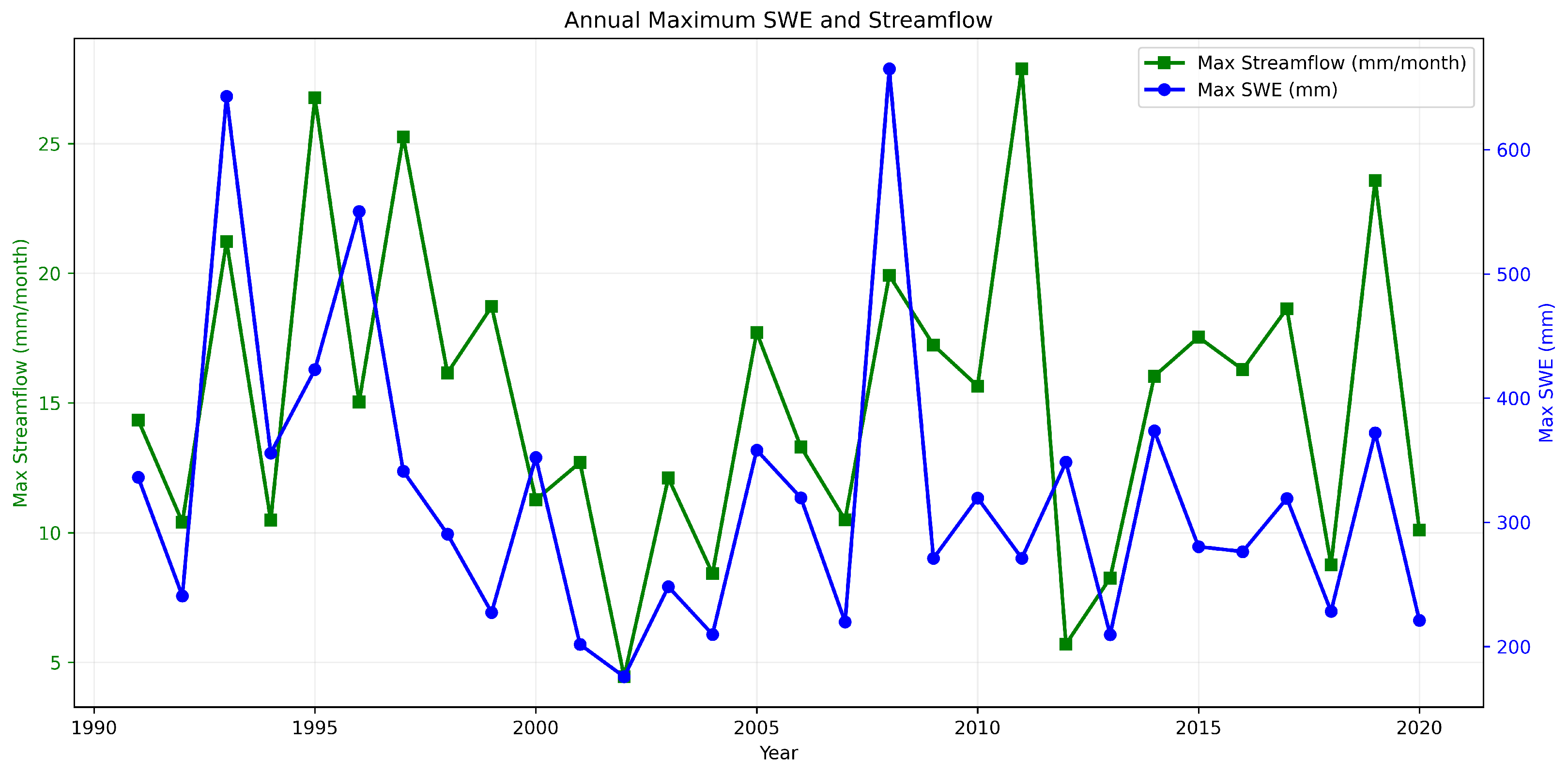
Figure 2 illustrates the time series of the annual maximum snow water equivalent (SWE) represented by the blue curve and streamflow depicted by the green curve, spanning the period from 1991 to 2020. The plot underscores significant interannual variability in snowpack within the UCRB, with notable peaks in the SWE, such as those observed in 1993 and 2008, corresponding to years characterized by elevated maximum streamflow. While the SWE demonstrates more pronounced fluctuations on an annual basis, the streamflow peaks exhibit a consistent yet lower magnitude seasonal maximum. These patterns underscore the SWE as a primary determinant of runoff in river basins dominated by snowmelt.

Figure 2. Annual max SWE and streamflow over time.

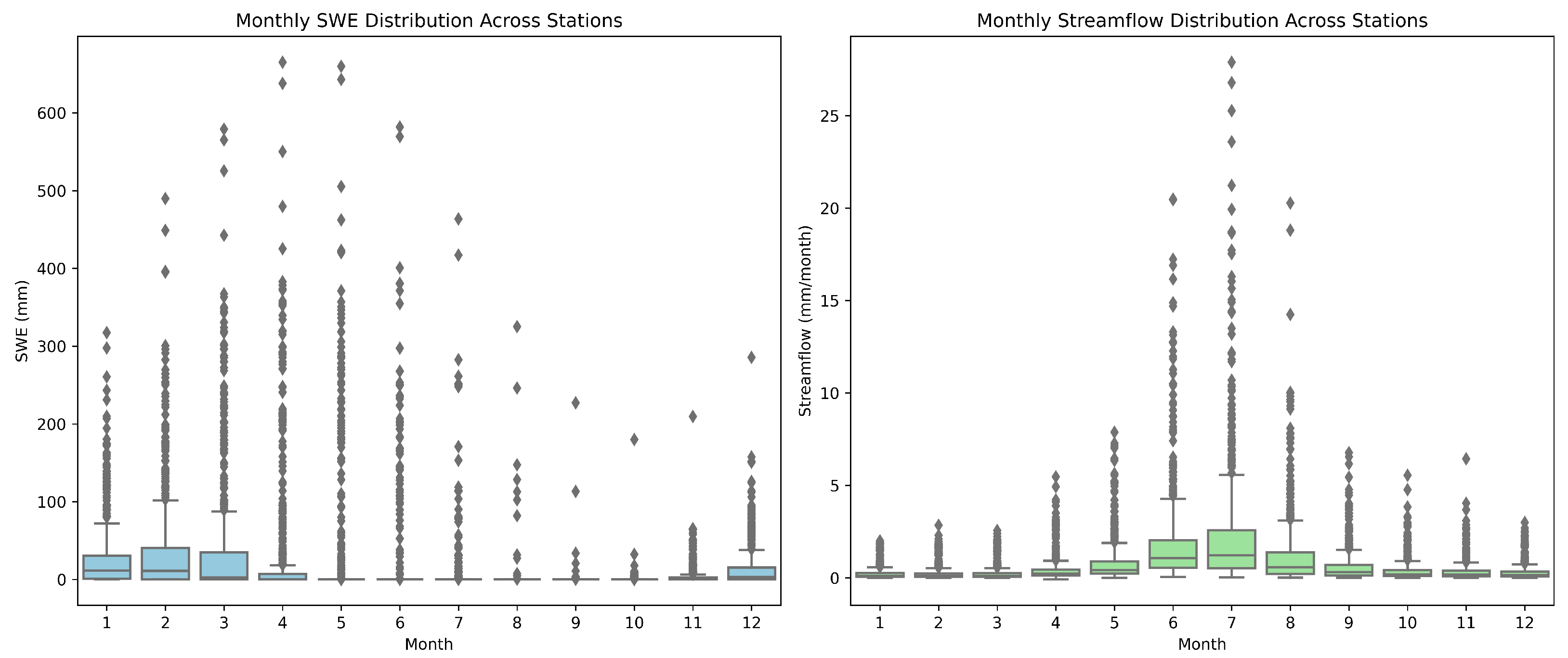
Figure 3 illustrates boxplots showing the aggregated monthly distributions of SWE (left panel) and streamflow (right panel) across 20 stations over the 30 years (1991–2020). The distribution of SWE exhibits a distinct seasonal cycle, reaching its peak between February and April, followed by a rapid decline during the summer and autumn months as snowpack melts. In contrast, streamflow reaches its maximum between May and July, demonstrating a typical lag between peak snow accumulation and subsequent runoff. The considerable range of observed SWE values during the peak months indicates spatial heterogeneity within the basin, which is attributable to variations in elevation and physiographic settings. The streamflow plot similarly captures this spatial variability, with certain stations experiencing significantly higher flows due to localized snowmelt contributions.

Figure 3. Monthly streamflow and SWE distribution across stations.

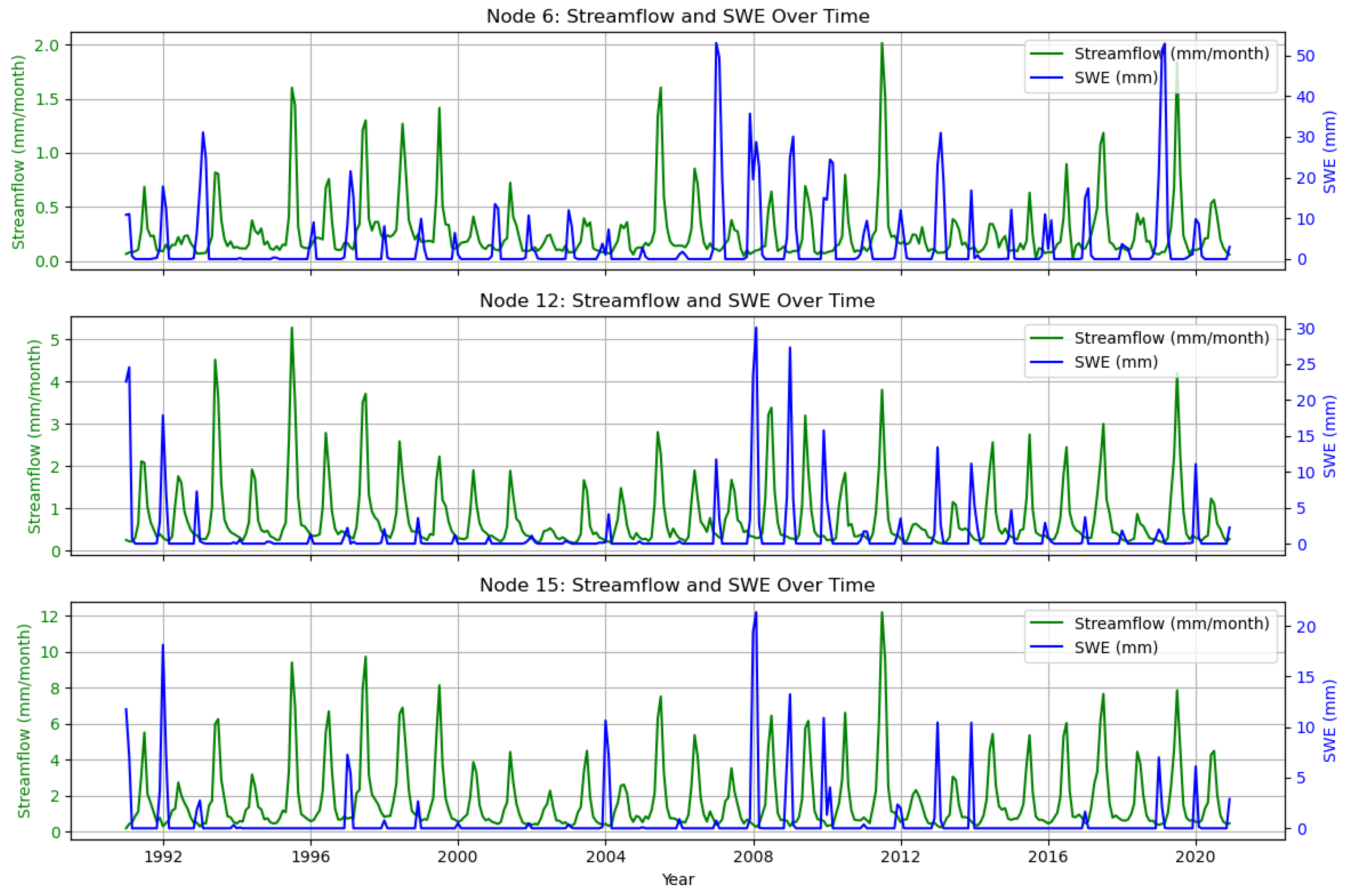
Figure 4 presents detailed time-series plots of the SWE (blue) and streamflow (green) for three representative stations: Node 6—Duchesne River Near Randlett, Utah; Node 12—Gunnison River Near Grand Junction, Colorado; and Node 15—Green River At Green River, Utah. These stations illustrate the concurrent evolution of snowpack and runoff across varying elevations within the basin. Node 6 (top panel), situated at a higher elevation, consistently displays SWE peaks that precede sharp rises in streamflow, typically observed in late spring to early summer. Node 12 (middle panel) exhibits similar seasonal dynamics but with lower magnitudes of both SWE and streamflow. In contrast, Node 15 (bottom panel) experiences minimal SWE accumulation, and its streamflow pattern reflects a more muted, rain-dominated response, underscoring the influence of local topography and climate.

Figure 4. SWE and streamflow over time.

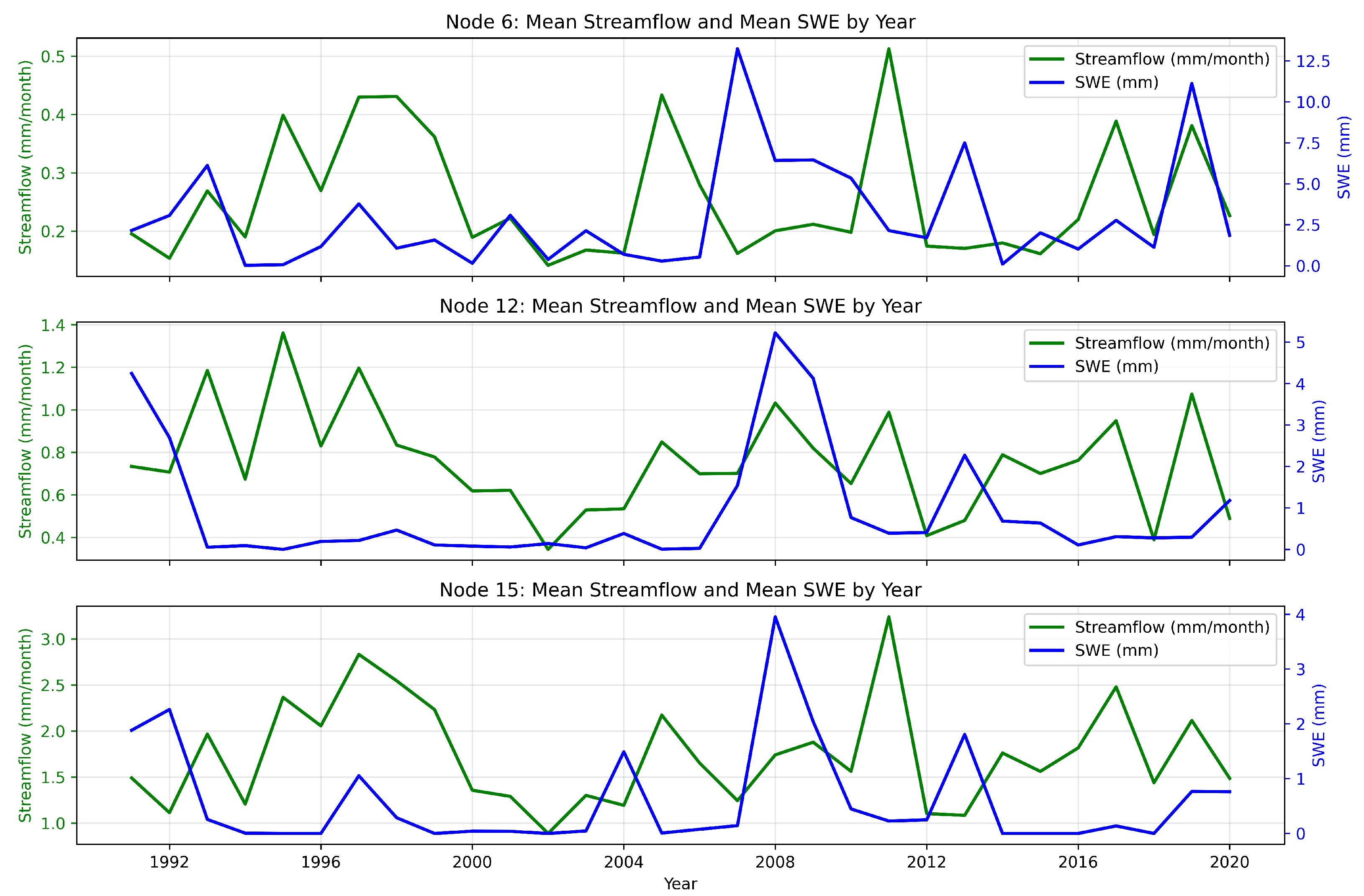
Figure 5 shows the corresponding annual mean SWE and streamflow for the same three stations. By aggregating the monthly records to yearly means, these plots emphasize interannual variability and long-term trends, complementing the seasonal dynamics shown in Figure 4.

Figure 5. Annual mean streamflow and SWE for a few nodes.

4. Methodology

This section provides an overview of the methodologies employed for streamflow forecasting. To prepare the dataset for model training, we applied Z-score normalization and constructed fixed-length input–output sequences. Each variable (streamflow and SWE) was normalized using the following formula:

$$x^{\prime }={\displaystyle \frac{x-\mu }{\sigma }}$$

(1)

where x is the original value, $\mu$ is the mean, and $\sigma$ is the standard deviation computed from the training set. This normalization was performed separately for each station to remove scale differences and stabilize model training.

As described in Section 3, the dataset spans from 1991 to 2020. The training set spans January 1991 to December 2009 (63.33% of the data), while the testing set covers January 2010 to December 2020 (36.67%). We adopted a sequence-to-sequence structure using a 36-month lookback window to predict the next 36 months of streamflow, capturing long-term dependencies and seasonal variations critical in snowmelt-driven basins. Overlapping sliding windows were used to generate input–output pairs across the full time series [40].

4.1. Long Short-Term Memory (LSTM)

LSTM networks are a specialized class of Recurrent Neural Networks (RNNs) designed to capture long-range dependencies in sequential data. Their ability to model nonlinear temporal dynamics makes them particularly effective for hydrological forecasting [24,26,41].

In this study, an LSTM model was developed to predict the monthly streamflow at multiple gauging stations. The model architecture consists of an input layer, a single hidden LSTM layer with 64 units, and a fully connected output layer. It follows a sequence-to-sequence design: a 36-month lookback window is used to predict the streamflow for the subsequent 36 months. The input features include lagged streamflow values and the SWE, allowing the model to integrate both autoregressive and snow-driven hydrological signals.

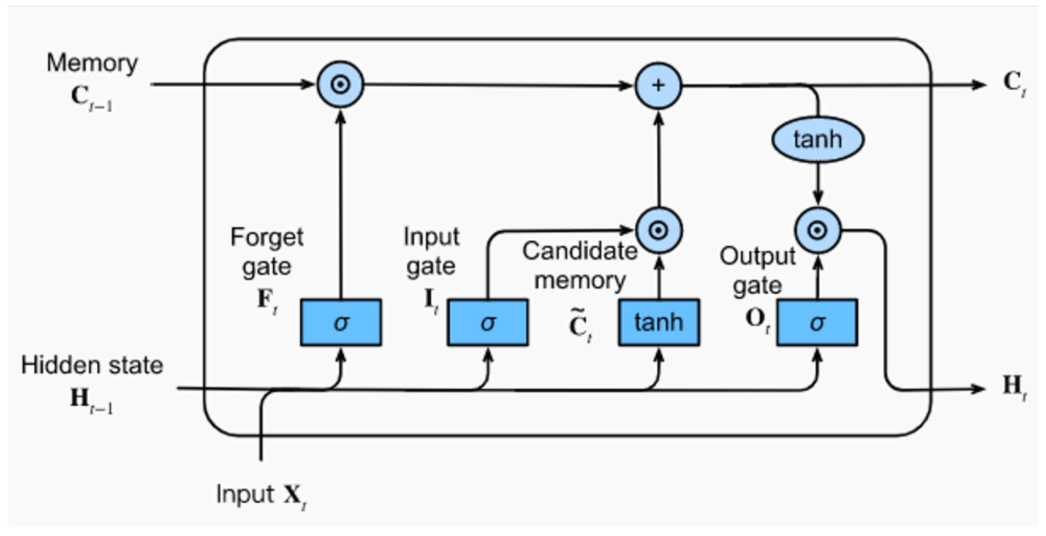
The core of the LSTM architecture is its memory cell, which maintains a cell state ($C_t$) regulated by three gating mechanisms—a forget gate ($f_t$), input gate ($i_t$), and output gate ($o_t$)—that modulate information flow. These operations are mathematically defined as

$$\begin{array}{cc}\hfill f_t& =\sigma (W_f[h_{t-1},x_t]+b_f)\hfill \end{array}$$

(2)

$$\begin{array}{cc}\hfill i_t& =\sigma (W_i[h_{t-1},x_t]+b_i)\hfill \end{array}$$

(3)

$$\begin{array}{cc}\hfill {\tilde{C}}_t& =tanh(W_C[h_{t-1},x_t]+b_C)\hfill \end{array}$$

(4)

$$\begin{array}{cc}\hfill C_t& =f_t\odot C_{t-1}+i_t\odot {\tilde{C}}_t\hfill \end{array}$$

(5)

$$\begin{array}{cc}\hfill o_t& =\sigma (W_o[h_{t-1},x_t]+b_o)\hfill \end{array}$$

(6)

$$\begin{array}{cc}\hfill h_t& =o_t\odot tanh\left(C_t\right),\hfill \end{array}$$

(7)

where, $\sigma$ denotes the sigmoid activation function, tanh represents the hyperbolic tangent function, ⊙ indicates element-wise multiplication, and W and b are learnable weights and biases. A schematic of the LSTM cell and its gating mechanisms is shown in Figure 6.

Figure 6. The structure of an LSTM memory unit [40,42].

These gating operations enable the LSTM to selectively retain long-term information while discarding irrelevant signals, enhancing its robustness in modeling complex hydrological processes.

Model training was conducted using TensorFlow and the Adam optimizer. Hyperparameters were selected via grid search, with the final configuration including a batch size of 32, learning rate of 0.001, 100 training epochs, and a single hidden LSTM layer with 64 units.

4.2. Gated Recurrent Unit (GRU)

The Gated Recurrent Unit (GRU), introduced by [43], is a simplified and computationally efficient alternative to an LSTM network. It was designed to address the vanishing gradient problem commonly encountered in traditional RNNs. GRUs rely on two gating mechanisms—the update gate and the reset gate—which regulate the flow of information through the network. In contrast to LSTMs that use separate input, forget, and output gates, GRUs streamline this process into a more compact and faster architecture while still preserving the ability to learn long-term dependencies in sequential data.

A GRU updates its hidden state according to the following equations:

$$\begin{array}{cc}\hfill z_t& =\sigma (W_z·[h_{t-1},x_t])\hfill \end{array}$$

(8)

$$\begin{array}{cc}\hfill r_t& =\sigma (W_r·[h_{t-1},x_t])\hfill \end{array}$$

(9)

$$\begin{array}{cc}\hfill {\tilde{h}}_t& =tanh(W·[r_t\ast h_{t-1},x_t])\hfill \end{array}$$

(10)

$$\begin{array}{cc}\hfill h_t& =(1-z_t)\ast h_{t-1}+z_t\ast {\tilde{h}}_t,\hfill \end{array}$$

(11)

where $z_t$ represents the update gate, which controls the extent to which the previous hidden state is carried forward, while $r_t$ is the reset gate, which determines how much of the past information to forget. The candidate hidden state (${\tilde{h}}_t$) is computed using the previous reset-modulated hidden state, and the final hidden state ($h_t$) is a convex combination of the previous and candidate states, weighted by the update gate.

In this study, GRU models were employed for both univariate and multivariate streamflow prediction tasks. The input sequence consisted of a 36-month look-back window, with each time step comprising two input features: streamflow and SWE. The GRU architecture included a single recurrent layer with 50 hidden units and a ReLU (Rectified Linear Unit) activation function defined as follows:

$$ReLU\left(x\right)=max(0,x)$$

(12)

It introduces non-linearity by outputting the input directly if it is positive; otherwise, it outputs zero [44]. This was followed by a fully connected dense layer that generates predictions over the forecasting horizon. To ensure a fair comparison with the LSTM model, the GRU was trained using the same configuration: 100 epochs, a batch size of 32, the Adam optimizer with a learning rate of 0.001, and mean squared error loss.

4.3. Seasonal Autoregressive Integrated Moving Average (SARIMA)

The SARIMA model is a classical and widely used approach for forecasting time-series data, particularly when strong seasonal patterns are present. SARIMA extends the ARIMA framework by incorporating seasonal autoregressive and moving average components, along with seasonal differencing, to capture both short-term dynamics and long-term seasonal cycles in the data. This makes it especially suitable for datasets recorded at regular intervals, such as monthly streamflow observations.

The general form of the SARIMA model is expressed as follows:

$$\begin{array}{cc}\hfill \mathrm{SARIMA}=& c+\sum _{n=1}^p{\alpha }_n{y}_{t-n}+\sum _{n=1}^q{\theta }_n{\epsilon }_{t-n}\hfill \\ \hfill & +\sum _{n=1}^P{\varphi }_n{y}_{t-mn}+\sum _{n=1}^Q{\eta }_n{\epsilon }_{t-mn}+{\epsilon }_t\hfill \end{array}$$

(13)

In this equation, p, d, and q represent the orders of the non-seasonal autoregressive, differencing, and moving average terms, respectively, while P, D, and Q are their seasonal counterparts. The m parameter indicates the number of time steps in one seasonal cycle, $y_t$ is the observed value at time t, and ${\epsilon }_t$ is the random error term.

In this study, the SARIMA model was applied for streamflow forecasting under both univariate and multivariate experimental setups. The model was trained using a 36-month input–output window, consistent with the other evaluated models. Based on performance tuning, the model that yielded the best results was configured with non-seasonal parameters of $p=3$, $d=0$, and $q=2$, along with seasonal parameters of $P=1$, $D=0$, and $Q=1$, assuming a seasonal period of 12 to account for monthly patterns. This parameterization captures both short-term dependencies and annual seasonal effects in the data. Notably, the absence of differencing in both the trend and seasonal components suggests that the input time series was already stationary, eliminating the need for additional transformation.

4.4. Random Forest Regression (RFR)

RFR is an ensemble learning model based on decision trees designed to enhance predictive accuracy and mitigate overfitting by aggregating the outputs of multiple decision trees (DTs). Each tree within the forest is trained on a distinct subset of the data through bootstrapping, and the final prediction is derived by averaging the predictions from all individual trees.

A simplified representation of the RFR model is depicted in Figure 7, where each decision tree has a depth of 2. This structure demonstrates how the ensemble synthesizes predictions from multiple shallow trees to yield a robust output. Mathematically, the RFR prediction is given by

$$\mathrm{RFR}\left(x\right)={\displaystyle \frac{1}{N}}\sum _{i=1}^N{T}_i\left(x\right),$$

(14)

where N is the total number of decision trees in the forest, $T_i\left(x\right)$ is the prediction from the $i^{\mathrm{th}}$ decision tree for input x, and $\mathrm{RFR}\left(x\right)$ is the final ensemble prediction.

Figure 7. A simplified structure of RFR.

We conducted extensive hyperparameter tuning to optimize the performance of the RFR model. The best results were achieved using the following configuration: number of estimators = 100, minimum samples required to split a node = 2, minimum samples required at each leaf node = 1, and bootstrapping enabled.

4.5. Spatio-Temporal Graph Neural Network (STGNN)

The proposed STGNN model integrates spatial and temporal modeling components to capture complex dependencies inherent in streamflow dynamics across multiple hydrological stations.

4.5.1. Graph Construction

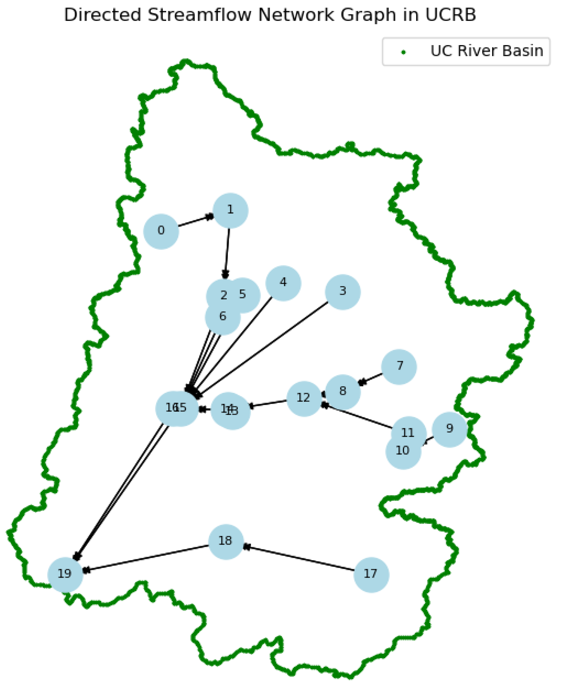
Let $V=\{v_1,v_2,\dots ,v_N\}$ represent the set of N hydrological stations, each corresponding to a United States Geological Survey (USGS) monitoring location within the UCRB as shown in Figure 8. The spatial relationships among these stations are encoded using an adjacency matrix ($A\in {\{0,1\}}^{N\times N}$) defined as follows:

$$A_{ij}=\left\{\begin{array}{cc}1,\hfill & \mathrm{if}\mathrm{station}{v}_i\mathrm{is}\mathrm{directly}\mathrm{connected}\mathrm{to}{v}_j\hfill \\ 0,\hfill & \mathrm{otherwise}\hfill \end{array}\right.$$

Figure 8. Directed streamflow network graph for the UCRB, with nodes representing hydrological stations and edges representing the flow directions between stations.

This connectivity is determined based on the hydrographic structure of the basin, ensuring that the adjacency matrix reflects the natural flow paths, including both main channels and tributaries. Stations sharing a river reach or located within the same sub-basin are considered neighbors. This graph representation preserves the directional hydrological influence from upstream to downstream stations, aligning with the physical topology of the basin [45,46,47].

4.5.2. Spatial Modeling with Graph Convolutional Networks (GCNs)

To model spatial dependencies, we employ GCNs, which enable each station to aggregate information from its immediate neighbors. The layer-wise propagation rule for the GCN is given by

$$H^{(l+1)}=\sigma \left(D^{-{\displaystyle \frac{1}{2}}}A{D}^{-{\displaystyle \frac{1}{2}}}{H}^{\left(l\right)}{W}^{\left(l\right)}\right),$$

(15)

where $H^{\left(l\right)}$ denotes the node feature matrix at layer l, A is the adjacency matrix, D is the degree matrix, $W^{\left(l\right)}$ is a trainable weight matrix, and $\sigma (·)$ represents a nonlinear activation function (e.g., ReLU). By stacking multiple GCN layers, the model captures increasingly complex spatial relationships, allowing each node embedding to reflect upstream and downstream influences through recursive neighbor aggregation [38].

4.5.3. Temporal Modeling with LSTM

The spatial embeddings produced by the GCN layers are reshaped into sequential inputs for an LSTM network, which models temporal dependencies. For each station, a sequence of historical embeddings over a defined input window of 36 months is passed to the LSTM. The LSTM updates its hidden $H_t$ and $C_t$ cell states at each time step (t), capturing both short-term fluctuations and long-term seasonal trends.

Upon processing of the entire sequence, the LSTM outputs a final hidden state ($H_{\mathrm{end}}$), which serves as a compact spatio-temporal representation of the station’s historical behavior.

4.5.4. Output Layer and Multi-Step Forecasting

The final prediction is generated by passing $H_{\mathrm{end}}$ through a fully connected (FC) layer:

$$\mathbf{Y}=\mathrm{FC}\left(H_{\mathrm{end}}\right)\in {\mathbb{R}}^{N\times p},$$

(16)

where N is the number of stations and p is the forecasting horizon (e.g., 12, 24, or 60 months). Dropout regularization may be applied after the FC layer to prevent overfitting and improve generalization, as recommended in recent literature on data-driven hydrological forecasting [47,48].

The complete workflow of the STGNN architecture is illustrated in Figure 9, highlighting spatial aggregation via GCN, temporal modeling using LSTM, and final multi-step prediction through the fully connected layer. For the STGNN, we used an input dimension equal to the number of features, a hidden dimension of 64, two graph convolutional layers, a dropout rate of 0.2, and a fully connected output layer. Training was conducted for 150 epochs with a batch size of 32, using the Adam optimizer with a learning rate of 0.001.

Figure 9. Architecture of the proposed STGNN.

4.6. Evaluation Metrics

To evaluate the performance of the streamflow prediction models in both univariate and multivariate setups, we employ a comprehensive set of regression-based and hydrologically relevant metrics. These include traditional measures such as Mean Absolute Error (MAE), Root Mean Square Error (RMSE), R-squared ($R^2$), Mean Absolute Percentage Error (MAPE), and Symmetric Mean Absolute Percentage Error (SMAPE), as well as hydrology-specific metrics such as Nash–Sutcliffe Efficiency (NSE) and Kling–Gupta Efficiency (KGE).

Let $x_i$ denote the observed values, $y_i$ represent predicted values, $\overline{x}$ be the mean of observed values, and n be the number of observations.

MAE measures the average magnitude of prediction errors without considering their direction.

$$\mathrm{MAE}={\displaystyle \frac{1}{n}}\sum _{i=1}^n|y_i-x_i|$$

(17)

RMSE quantifies the average squared deviation between predicted and observed values, penalizing larger errors more.

$$\mathrm{RMSE}=\sqrt{{\displaystyle \frac{1}{n}}\sum _{i=1}^n{(y_i-x_i)}^2}$$

(18)

$R^2$ measures how well the model’s predictions match the variability in the observed data, with 1 representing perfect prediction.

$$R^2=1-{\displaystyle \frac{{\sum }_{i=1}^n{(y_i-x_i)}^2}{{\sum }_{i=1}^n{(x_i-\overline{x})}^2}}$$

(19)

MAPE provides a percentage-based error measure but may be unstable when $x_i$ approaches zero.

$$\mathrm{MAPE}={\displaystyle \frac{100}{n}}\sum _{i=1}^n\left|{\displaystyle \frac{y_i-x_i}{x_i}}\right|$$

(20)

SMAPE addresses the asymmetry and scale sensitivity issues of MAPE by normalizing against the average magnitude.

$$\mathrm{SMAPE}={\displaystyle \frac{100}{n}}\sum _{i=1}^n{\displaystyle \frac{|y_i-x_i|}{\left(\right|y_i|+|x_i\left|\right)/2}}$$

(21)

NSE [49], commonly used in hydrology, compares model predictions to the mean of observations. Values closer to 1 indicate better performance.

$$\mathrm{NSE}=1-{\displaystyle \frac{{\sum }_{i=1}^n{(x_i-y_i)}^2}{{\sum }_{i=1}^n{(x_i-\overline{x})}^2}}$$

(22)

KGE [50] jointly assesses correlation, variability, and bias, making it suitable for hydrological evaluations.

$$\mathrm{KGE}=1-\sqrt{{(r-1)}^2+{(\alpha -1)}^2+{(\beta -1)}^2}$$

(23)

where r is the Pearson correlation coefficient between x and y, $\alpha ={\displaystyle \frac{{\sigma }_y}{{\sigma }_x}}$ (variability ratio), and $\beta ={\displaystyle \frac{\overline{y}}{\overline{x}}}$ (bias ratio).

5. Results

This section presents a comprehensive evaluation of various models for streamflow prediction over the Lees Ferry region of the UCRB. The experiments are organized into the following three subsections:

• Model performance comparison under univariate and multivariate settings;
• Seasonal analysis of model predictions;
• Generalization performance across the entire basin.

We use a fixed configuration of 36 months of historical input and a prediction horizon of 36 months, as determined in prior work [40]. Multivariate models utilize both streamflow and SWE as inputs, while univariate models rely solely on streamflow data.

5.1. Model Performance Comparison

Table 1 displays the comparative results for the five models—GRU, LSTM, SARIMA, RFR, and STGNN—across the univariate and multivariate setups. The evaluation is based on key hydrological performance metrics: NSE, R², MAE, KGE, and RMSE.

Table 1. Performance of models at Lees Ferry (univariate vs. multivariate).

Type	Model	NSE	R2	MAE	KGE	RMSE
Univariate	GRU	0.66	0.66	1.76	0.54	2.71
	LSTM	0.34	0.35	2.36	0.57	3.76
	SARIMA	0.17	0.17	2.28	0.52	4.24
	RFR	0.74	0.74	1.52	0.49	2.38
	STGNN	0.79	0.79	0.31	0.81	0.78
Multivariate	GRU	0.69	0.69	1.65	0.50	2.57
	LSTM	0.55	0.55	2.12	0.55	3.09
	SARIMA	0.28	0.28	2.18	0.52	3.95
	RFR	0.70	0.70	1.63	0.44	2.56
	STGNN	0.84	0.84	0.29	0.84	0.68

These results indicate that including the SWE in the input feature set improves model performance overall. The transition from univariate to multivariate inputs yielded higher NSE values and reduced error metrics (MAE and RMSE), while KGE improvements were more variable across stations. The most significant improvements were observed in the GRU and STGNN models. This enhancement can be attributed to the added predictive power of the SWE, which serves as a proxy for snowpack dynamics, a key driver of streamflow variability in the UCRB.

The STGNN model demonstrated the highest overall performance in both univariate and multivariate settings, achieving an NSE of 0.84 and KGE of 0.84 in the multivariate configuration, substantially outperforming all other models. Its superior performance is primarily due to its ability to learn both spatial and temporal dependencies within the river network. Unlike conventional sequence models that process time-series data in isolation, STGNN leverages a graph-based structure that encodes the topological relationships between different streamflow gauges. This architecture enables the model to incorporate upstream and downstream influences and spatial correlations, which are particularly important in hydrologically connected systems. Prior work has shown that incorporating spatial dependencies through graph-based learning improves both the stability and accuracy of hydrological forecasts, especially in basins characterized by complex terrain and snow-dominated regimes [40].

Models such as GRU and RFR also showed improvements in the multivariate setting, with GRU’s NSE increasing from 0.66 to 0.69 and RFR maintaining a high level of performance (0.74 to 0.70 NSE) while slightly improving its error metrics. These models can capture nonlinear relationships between input variables and output streamflow, and the availability of SWE enhances their capacity to model the physical processes underlying streamflow generation. In the case of GRU, its gated recurrent architecture enables it to retain long-term dependencies, which are crucial for modeling delayed runoff caused by snow accumulation and melt. The addition of the SWE appears to provide sufficient context to improve the learning of such lagged hydrological responses.

In contrast, the SARIMA and LSTM models showed relatively limited improvement when the SWE was introduced. SARIMA, being inherently linear and univariate in nature, is not well suited for modeling complex, nonlinear processes or handling multiple input variables. Even in its extended form, the model cannot effectively learn the interactions between the SWE and streamflow without manual specification of lags or exogenous structures. Similarly, while LSTM is theoretically capable of handling multivariate sequences, its performance remains suboptimal. Although NSE improved from 0.34 to 0.55, this is still below the accuracy achieved by GRU and STGNN, reflecting LSTM’s inability to model spatial dependencies and its higher sensitivity to noise in long input sequences. The lack of spatial awareness makes LSTM vulnerable to overfitting and poor generalization, particularly when dealing with heterogeneous inputs across different seasons or flow regimes.

The STGNN model, in comparison, integrates both the temporal dimension (through recurrent or convolutional layers) and the spatial dimension (via graph convolutions), enabling it to simultaneously capture the influence of snowpack variability and basin topology. This dual encoding is critical for achieving robust performance in snow-dominated basins, as streamflow at any given location is not solely a function of local conditions but also influenced by upstream snow accumulation and routing processes.

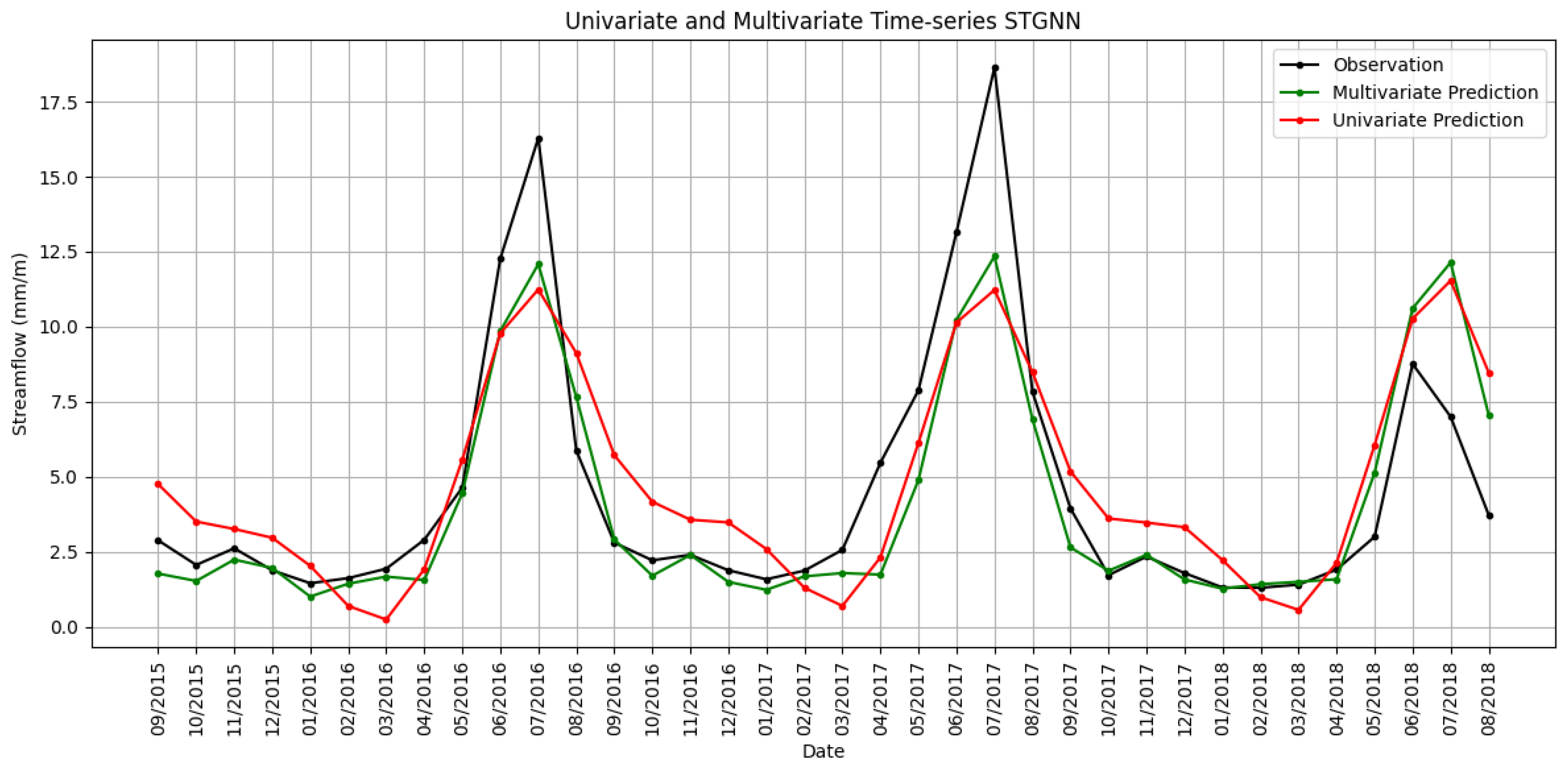
Figure 10 provides a clear visual comparison between observed streamflow at Lees Ferry and predictions made by both the univariate and multivariate versions of the STGNN model. The observed values, shown as a black line, reflect the actual streamflow measurements over several years, including both high-flow and low-flow periods. Superimposed on this are the model predictions: the red line represents the univariate STGNN, which relies solely on past streamflow observations from Lees Ferry itself, while the green line represents the multivariate STGNN, which incorporates additional inputs such as SWE and streamflow data from upstream nodes.

Figure 10. Univariate and multivariate time-series STGNN.

A close examination of the graph reveals that the multivariate STGNN consistently tracks observed flows more accurately than the univariate counterpart. This distinction is most evident during peak flow periods, typically associated with spring and early summer snowmelt, where observed streamflow rises sharply. In these intervals, the multivariate model mirrors both the magnitude and timing of high flows, whereas the univariate model tends to underestimate the peaks and, at times, lags behind in capturing the true pattern of the hydrograph. This improved correspondence underscores the value of integrating the spatially distributed SWE, which serves as a proxy for snowpack conditions and provides crucial information that cannot be extracted from local streamflow data alone.

Similarly, during periods of lower flow, both models are generally able to represent the overall shape and fluctuations of the observed series. However, the multivariate STGNN still outperforms the univariate model, maintaining closer alignment with the observed minima and better capturing the subtle seasonal and interannual dynamics of the river. This enhanced performance is a direct consequence of the model’s ability to assimilate upstream conditions, reflecting the physical reality that streamflow at Lees Ferry is greatly influenced by hydrological processes occurring throughout the basin—most notably, the accumulation and subsequent melting of snow at higher elevations.

The visual findings from this plot are in full agreement with the quantitative results presented in Table 1. Metrics such as NSE, KGE, MAE, and RMSE all exhibited marked improvements for the multivariate STGNN model relative to the univariate version and to other baseline models. These improvements are particularly pronounced for the STGNN, which is specifically designed to learn both temporal and spatial dependencies using graph-based neural network architectures. Such models are uniquely positioned to capture the interconnectedness of river networks and the propagation of upstream hydrological signals.

5.2. Seasonal Analysis

To gain further insight into the predictive stability and robustness of the models across different hydrological conditions, we conducted a seasonal analysis of their performance. A calendar year was divided into four hydrologically meaningful seasons based on dominant processes in the UCRB as shown in Table 2.

Table 2. Seasonal classification in the UCRB.

Season	Months	Description
Snow Accumulation	November–February	Winter period characterized by low flows and dominant snow storage.
Melt	March–May	Transitional period where rising temperatures initiate partial snowmelt.
High Flow	June–August	Peak discharge season driven by extensive snowmelt runoff.
Base	September–October	Early autumn period where flows stabilize before winter onset.

This classification allows us to evaluate model sensitivity to seasonal variations in snow accumulation and melt, which are key drivers of streamflow in snow-dominated basins like the UCRB.

5.2.1. RMSE Distribution Across Models

Figure 11 presents violin plots of RMSE distributions for each model under both univariate (yellow) and multivariate (green) input conditions. The x mark within each distribution denotes the median RMSE value for that model and setting.

Figure 11. RMSE distribution across models (univariate vs. multivariate).

The RMSE distributions provide several important insights. First, across nearly all models, the multivariate configurations exhibit narrower distributions than their univariate counterparts. This pattern suggests that the inclusion of the SWE as an additional predictor improves not only the average accuracy but also the consistency of predictions across different seasonal and hydrological regimes. This finding aligns with prior literature highlighting that incorporating snowpack-related variables helps reduce predictive variance in snow-fed basins [29,51].

For models such as GRU, RFR, and especially STGNN, the RMSE distributions are not only compact but also centered around lower median values. For instance, STGNN shows a tight distribution in both settings, with only a marginal decrease in spread in the multivariate case, suggesting stable performance across seasonal shifts and sub-basin variability. This low variance in predictive error is a hallmark of models capable of generalizing well over different input regimes.

In contrast, LSTM and SARIMA display broader and more dispersed RMSE distributions, particularly in the multivariate setting for LSTM and the univariate setting for SARIMA. These results indicate higher sensitivity to input variation and possible overfitting or underfitting issues, depending on the complexity of the season-specific flow regimes. LSTM’s wide spread in the multivariate case suggests that while the model has the capacity to learn from the SWE, it may lack sufficient regularization or spatial awareness to fully leverage this input across all seasons. SARIMA’s behavior further confirms its limitation as a linear model in capturing nonlinear and process-driven data.

5.2.2. STGNN Seasonal NSE Improvement

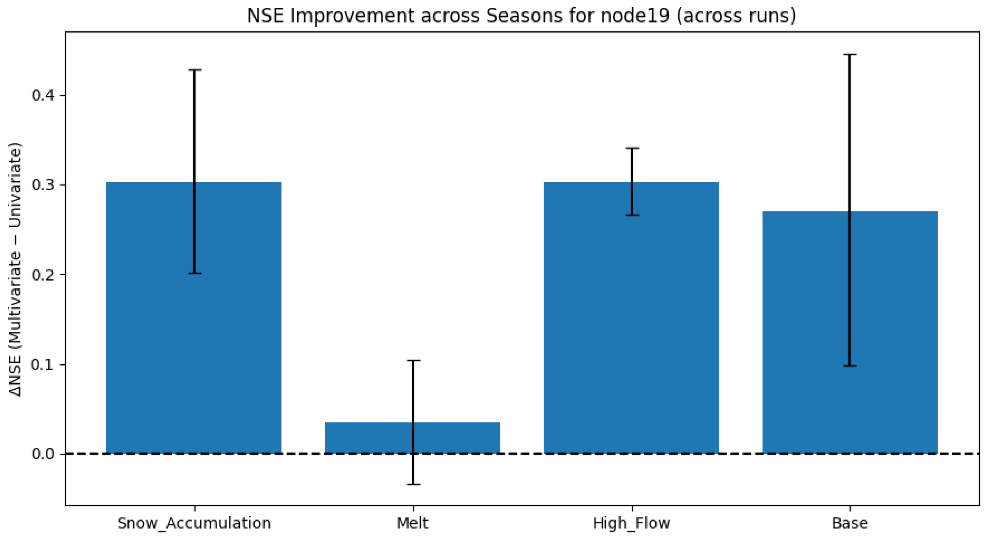
Figure 12 plots the seasonal difference in NSE between the multivariate and univariate models at Lees Ferry. Bars show the mean across independent training replicates, and whiskers indicate 95 percent confidence intervals.

Figure 12. NSE improvement across seasons for Node 19.

The model shows a substantial and statistically reliable improvement when the SWE is included, with confidence intervals clearly above zero in the snow accumulation season. Active snowpack development in the high-elevation headwaters creates strong spatial gradients in storage. Incorporating the spatially distributed SWE allows the model to represent this heterogeneity and its evolution, which constrains initial conditions that shape later runoff reaching the outlet. The consistently positive improvement indicates a robust signal. From March through May, the mean effect of the SWE is small, and its confidence interval overlaps zero. By this time, the local SWE near the outlet is typically negligible because Lees Ferry sits at a lower elevation than the contributing headwaters, and the rain and snow transition can shift rapidly. These factors reduce the informativeness of the gridded SWE for month-to-month discharge at the outlet, so modest improvements or slight degradations can occur, depending on hydroclimatic conditions.

High-flow months present the largest mean gain, with confidence intervals that are clearly positive. This reflects delayed meltwater from high-elevation headwaters dominating the hydrograph at Lees Ferry. Using the SWE from all upstream nodes helps capture the basin’s integrated snowmelt signal in terms of both timing and magnitude, which a univariate baseline cannot infer from discharge history alone. The agreement across independent replicates shows this benefit is large and stable. In base flow months, the mean improvement is positive, but the confidence interval is wide, indicating greater variability between model realizations. With snowpack largely absent, processes other than snow, such as groundwater contributions, soil moisture memory, and antecedent rainfall, govern low flows at the outlet. The SWE can still help indirectly in some years, which explains the positive mean, but the broad interval cautions that the magnitude of the gain is uncertain.

5.2.3. MAE Comparison

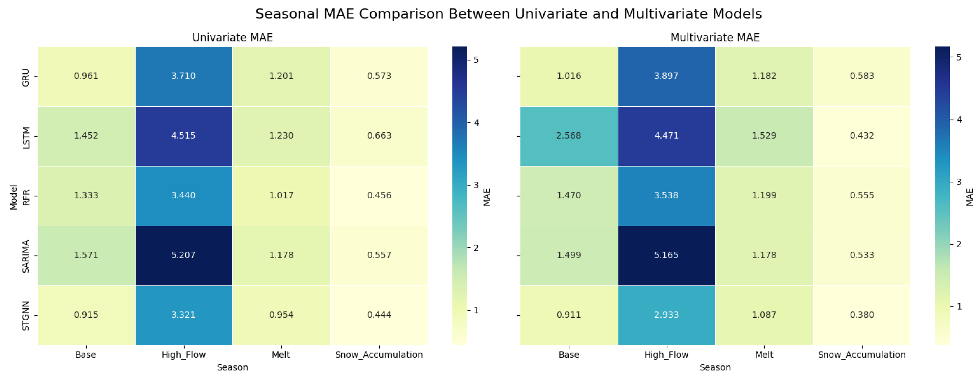
The seasonal comparison of MAE highlights the strong dependence of model performance on dominant hydrological processes, with distinct behavior observed across the snow accumulation, melt, high-flow, and base-flow periods. The results reveal that model accuracy is not uniform throughout the year, and performance variations align closely with seasonal shifts in snowpack dynamics and runoff generation (Figure 13).

Figure 13. Seasonal MAE comparison across nodes.

During the high-flow season (June–August), which is primarily driven by snowmelt, all models exhibit their highest error magnitudes. In this period, univariate model MAEs cluster between approximately 3.3 and 5.2 m³/s, reflecting the challenges in capturing rapid streamflow changes arising from nonlinear melt processes, spatial heterogeneity in snow distribution, and energy balance dynamics. Notably, the multivariate models achieve the most substantial improvements during this season, as the inclusion of the SWE helps models better capture the snowmelt–streamflow relationship. Among them, the STGNN model demonstrates the largest reduction in MAE, dropping from approximately 3.32 m³/s in the univariate setting to 2.93 m³/s in the multivariate configuration. This result underscores STGNN’s ability to integrate both temporal dynamics and spatially structured state information for improved seasonal performance.

In contrast, during the base flow period (September–October), when streamflow is relatively stable and influenced less by snowmelt, the benefit of multivariate inputs diminishes. In some cases, adding the SWE appears to slightly degrade model accuracy—for example, GRU’s MAE increases from 0.96 to 1.02 m³/s and LSTM’s from 1.45 to 2.57 m³/s. These increases suggest that during hydrologically quiescent months, the additional complexity introduced by auxiliary variables may introduce noise or lead to overfitting rather than offering predictive value.

The snow accumulation (November–February) and melt (March–May) seasons show more mixed behavior. While models like GRU and STGNN exhibit modest improvements in MAE under multivariate configurations, other models (such as LSTM and SARIMA) show little to no benefit. This variability suggests that while the inclusion of the SWE can help capture early signs of runoff or internal catchment state, not all models are equally equipped to leverage this information effectively.

5.3. Generalization of STGNN Performance Across the Basin

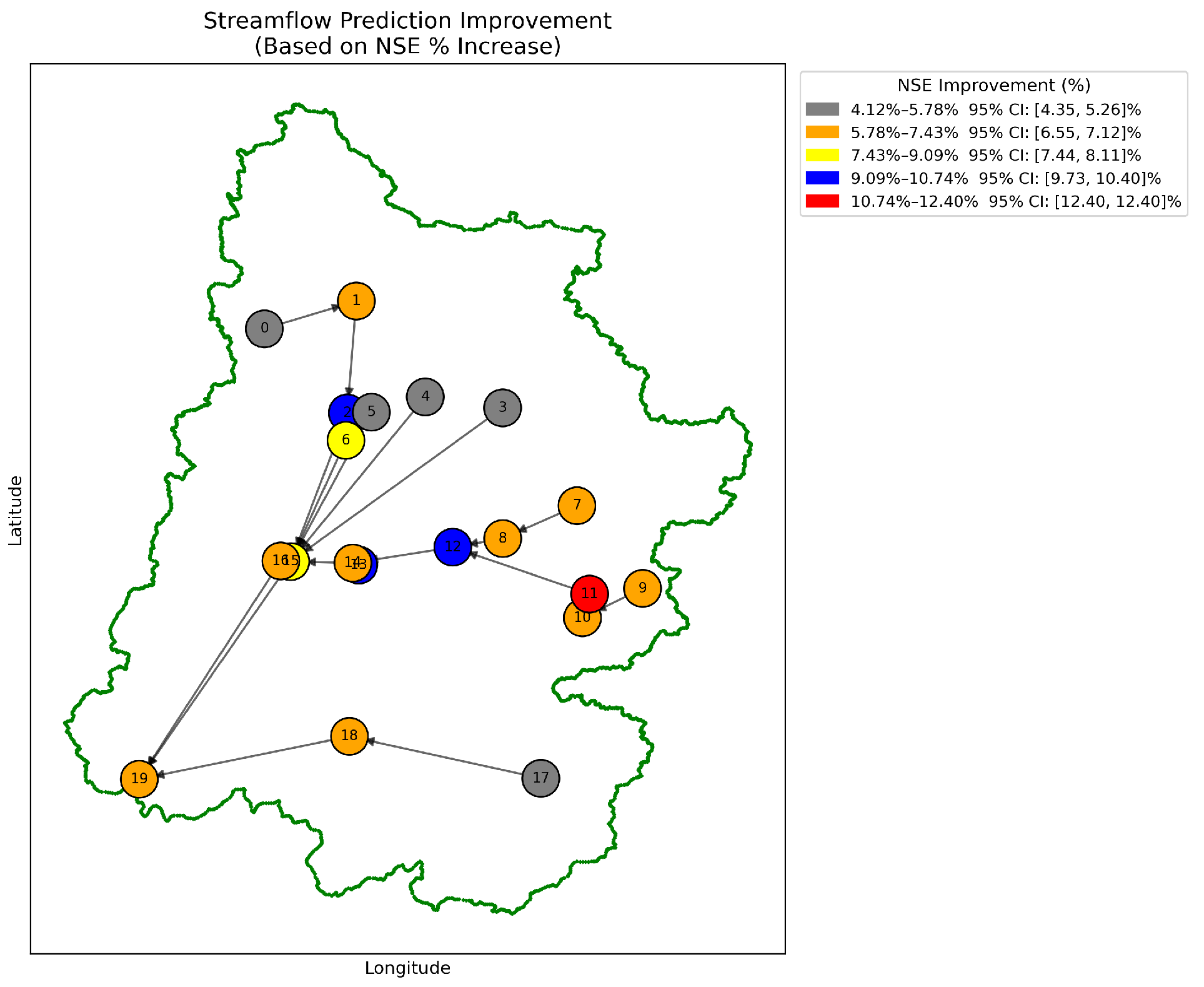
Figure 14 provides a spatial overview of NSE improvement across all 20 gauging stations after incorporating SWE data. Each node is color-coded based on its relative improvement, with arrows showing flow direction and the basin boundary shown in green.

Figure 14. Streamflow prediction improvement.

As seen in Figure 14, stations in the interior and higher elevation zones tend to exhibit larger performance gains (blue to red colors), while headwater and low-lying stations show more modest improvement (gray to yellow). To better understand these differences, we evaluate the patterns by NSE improvement category, elevation, and network position.

5.3.1. NSE Improvement Categories and Headwater Behavior

Headwater stations—those without any upstream inflows—are over-represented in the minimal category. As shown in Table 3, five out of the seven headwater nodes experienced less than 5.8% improvement in NSE. This suggests that the absence of upstream snowpack information limits the capacity of SWE data to enhance predictions in these areas, even in cases where the local elevation is high.

Table 3. NSE improvement categories across all stations.

Category	NSE Improvement (%)	Stations (n)	$\mathbf{\Delta }$NSE (%) [95% CI]	Characteristic Features
Minimal	4.12–5.78	5	4.80 [4.35, 5.26]	Predominantly headwater locations
Low	5.78–7.43	9	6.87 [6.55, 7.12]	Mostly low-elevation stations
Moderate	7.43–9.09	2	7.78 [7.44, 8.11] †	Typically mid-network locations
High	9.09–10.74	3	9.98 [9.73, 10.40]	Mid- to high-elevation stations
Very High	10.74–12.40	1	12.40 [12.40, 12.40] †	Exclusively high-elevation sites

Note. Values are group means with 95% percentile-bootstrap CIs across stations (5000 resamples). ^† CIs are approximate due to very small n values (for n = 1, the interval collapses to a point).

5.3.2. Elevation Dependence of NSE Improvement

Elevation exhibited a strong influence on SWE effectiveness. Stations were grouped into three elevation bands: High (>3000 m), Mid (1500–3000 m), and Low (<1500 m). The average elevation and typical NSE improvement range within each band are provided in Table 4.

Table 4. NSE improvement by elevation band.

Elevation Band (m)	Stations (n)	Mean Elevation (m)	$\mathbf{\Delta }$NSE (%) [95% CI]	Typical NSE Gain Category
High (>3000)	2	3266	9.74 [7.08, 12.40]	High to very high
Mid (1500–3000)	10	1946	6.21 [5.22, 7.43]	Moderate to high
Low (<1500)	8	1330	7.76 [6.93, 8.76]	Minimal to low

Stations above 3000 m achieved the greatest NSE improvements, driven by deep and variable snowpack, which made the SWE a particularly informative predictor. Mid-elevation stations, occupying the rain–snow transition zone, also showed substantial gains, as SWE helped refine the timing and magnitude of snowmelt-driven runoff. In contrast, low-elevation stations dominated by rainfall processes exhibited limited improvement, as the SWE contributed little additional information to the models.

5.3.3. Influence of Network Position and Inflow Complexity

In addition to elevation, network topology also shaped model performance gains. Stations were categorized into three types based on their inflow structure: headwater, mid-network, and low-confluence. Summary statistics are shown in Table 5.

Table 5. NSE Improvement by stream network position.

Station Type	Typical Number of Inflows	NSE Gain Category	$\mathbf{\Delta }$NSE (%) [95% CI]
Headwater	0	Minimal	6.25 [5.26, 7.34]
Mid-network	≥3	Moderate to high	7.58 [7.05, 8.11]
Low-confluence	1–2	Low to moderate	8.26 [6.89, 9.84]

Headwater stations consistently experienced minimal gains due to their isolation from upstream snowpack contributions. In contrast, mid-network stations receiving flow from multiple tributaries benefited more substantially. The SWE data provided spatially aggregated snowmelt information that enhanced prediction accuracy in these nodes. Low-confluence stations showed intermediate improvement levels, likely because mixed hydrological inputs from both snow and rain reduced the relative influence of the SWE.

6. Discussion

The results from this study show that incorporating SWE data significantly enhances streamflow prediction accuracy in snow-affected basins such as the UCRB. This finding concurs with previous studies emphasizing the critical role of snowpack dynamics in controlling runoff timing and magnitude in mountainous watersheds [1,6]. Models that explicitly integrate the SWE as a predictor, especially when combined with upstream hydrological information, outperform those relying solely on local streamflow records, consistent with findings reported in [51,52].

Among the tested models, STGNN exhibited the highest predictive skill in both univariate and multivariate frameworks. The superior performance of STGNN underscores the importance of capturing both temporal sequences and spatial dependencies reflected in river network topologies, extending the principles shown in [53]. This graph-based architecture enables effective encoding of upstream influences, mimicking physical river-routing processes, thereby addressing inherent limitations of conventional sequence models that process time series independently [54].

The limited improvements seen with SARIMA and LSTM models align with prior critiques of these approaches in complex hydrologic settings. SARIMA’s linear structure restricts its ability to capture nonlinear snowmelt–streamflow dynamics [50], while LSTM’s lack of spatial context reduces its efficacy in representing spatial heterogeneity in snow distribution and melt timing [26]. The recurrent architecture of GRU allowed for moderate gains, thanks to improved temporal dependency modeling, corresponding with results from Choi et al. [55], who highlighted GRU’s robustness in hydrological modeling with lagged inputs.

Seasonal analysis revealed distinct patterns. The incorporation of the SWE substantially improved model skill during snow accumulation and high-flow seasons. This aligns with the conceptual understanding that snow accumulation governs basin storage capacity, while snowmelt runoff drives peak flows [56,57]. The notable NSE increases during high-flow season reaffirm that spatially distributed snowpack information is crucial for streamflow forecasting during peak runoff periods [58]. On the other hand, minimal or negative improvements during the melt and base seasons reflect the diminishing hydrological influence of snowpack as it depletes and other processes like groundwater or rainfall-driven flows dominate, echoing observations from [59].

The spatial heterogeneity in NSE improvement highlights the critical roles of elevation and network position. Consistent with prior research [60,61,62], high-elevation stations exhibited greater predictive gains due to deeper and more dynamic snowpacks, whereas low-elevation sites showed minimal benefits, reflecting their rain-dominated hydrology. Network topology further influences model utility; mid-network stations with multiple upstream tributaries benefited from richer spatial snowmelt signals, while headwater sites lacked such spatial context, limiting the SWE’s predictive power [63,64].

These findings emphasize that hydrological models for snow-dominated basins must move beyond uniform approaches and instead adopt physiographically aware frameworks that dynamically adjust to spatial and temporal heterogeneity [2,58]. Adaptive model architectures like STGNN provide a promising avenue to incorporate evolving hydrological states and basin connectivity, improving predictive reliability and informing water resource management under changing climate conditions [1,61].

7. Conclusions

This study shows that the integration of Snow Water Equivalent (SWE) and spatially distributed streamflow data into advanced hydrological models significantly enhances the prediction of river discharge in snow-dominated basins such as the Upper Colorado River Basin. Among all evaluated models, the Spatio-Temporal Graph Neural Network (STGNN) consistently achieved superior performance by effectively leveraging both temporal and spatial dependencies within the river network. The incorporation of the SWE was shown to improve model accuracy, particularly during critical periods of snow accumulation and high flow, when snowpack dynamics most strongly influence basin hydrology. These improvements align with and extend prior research, underscoring the necessity of context-aware, physically informed modeling frameworks for reliable streamflow forecasting in complex mountain watersheds.

The analysis also highlights the pronounced influence of elevation and network position on model gains from SWE integration. High-elevation and mid-network stations benefited most from spatially explicit snow information, while lower elevation and headwater stations exhibited weaker improvements. Importantly, the seasonal breakdown revealed that the utility of multivariate inputs such as the SWE is inherently time-dependent, with the greatest gains realized when snowpack processes are dominant and diminishing returns once local and upstream snow has been depleted. These findings advocate for adaptive, physiographically informed modeling approaches that adjust to both spatial and seasonal hydrological variability, ultimately supporting more robust operational water management and decision-making in snow-impacted regions.

While the present study advances the integration of the SWE and spatial context into machine learning based streamflow forecasting, several avenues remain for future research. One promising direction is the extension of these modeling frameworks to explicitly account for additional predictors, such as remote sensing-derived snow metrics, soil moisture, land cover changes, or meteorological forcings. Expanding the feature set may further clarify process linkages and improve model robustness under nonstationary climate conditions. Moreover, future work should explore model generalization and transferability across ungauged or data-sparse basins to assess scalability.