Abstract
Given significant water scarcity events in the recent past, water resources management in the Piracicaba River Basin, São Paulo, Brazil, has intensified the adoption of complex measures to meet the population’s water supply demands. This study presents a methodology to optimize reservoir water release while adhering to restrictive rules, aiming to also conserve water. A rainfall–runoff model was utilized alongside a hydrological routing model, incorporating meteorological forecasts for simulation over ten consecutive years. The results demonstrated significant water savings when comparing the optimization scenario with the actual reservoir operation during the same period. The applied methodology reduced water releases up to 66% in comparison to the observed scenario. Overall, the study introduces tools to improve reservoir operation with computational techniques, enriching local water resources management, water security, and decision-making processes, ensuring water security for the São Paulo Metropolitan Region, the most populous region in Brazil.
1. Introduction
Ensuring water supply and its allocation for diverse and conflicting uses represents a well-known and extensively explored issue in the fields of water resources management and hydrology. Water demands are continually increasing, compounded by the challenges of allocation and the influence of frequent climatic variations, which cause abrupt changes in hydrological regimes and create uncertainty in future water availability [1]. Severe water scarcity already affects two-thirds of the global population for at least one month annually, with nearly half of those impacted residing in India and China—regions where excessive withdrawals and degraded water quality compound the crisis [2,3]. When water quality factors are included, the percentage of the global population facing severe scarcity rises from 30% to 40%, underscoring the urgent need for resilient reservoir operations worldwide, especially under intensifying climate variability.
Recent studies have advanced the understanding of future water availability by simulating climate change scenarios using projections from Global Circulation Models (GCMs) and Earth System Models (ESMs), particularly those from CMIP5/SRES and CMIP6/SSP frameworks [1,4,5]. These works commonly apply hydrological models (such as MHD-INPE, SMAP, and SWAT+) to translate climate-driven changes in precipitation and evapotranspiration into long-term streamflow estimates, supporting assessments of water stress and system vulnerability. For instance, Ref. [4] evaluated system sustainability through performance metrics (Reliability, Resilience, and Vulnerability) across specific warming levels, while [1] integrated SWAT+ with Blue Water Scarcity and Vulnerability indices to quantify the probabilistic mismatch between water demand and supply. Ref. [5] adapted the SMAP model for a data-scarce basin, using flow percentiles (like the 95th percentile Q95%) and long-term mean outflow QLTM to estimate future resource reductions. In contrast to long-term projections, Ref. [6] introduced a short-term, risk-based decision-making framework for dam operations using ensemble rainfall forecasts to support preliminary water release, while [7] emphasized the dominant role of human interventions—such as dam construction—in altering flow regimes, underscoring the need for adaptive management. These approaches highlight the importance of integrating predictive tools at appropriate time scales and operational realities to improve water system responsiveness under climate variability. Despite advancements, there remains a need to integrate the technical contributions of the scientific community, which highlights relevant discussions on natural changes and their impact on the water cycle, with the empirical practices of regional water resource management, which still relies on subjective rules to manage water supply systems. Improving management requires determining and prioritizing strategies that promote more efficient use of water resources [8].
The Metropolitan Region of São Paulo (MRSP), due to its economic significance for Brazil and notable population density, requires a rigorous water supply system with multiple objectives. The Cantareira System is a regional complex comprising five reservoirs: Jaguari, Jacareí, Cachoeira, Atibainha, and Paiva Castro. With a total capacity of 33 m3s−1, the reservoir complex serves the MRSP, as well as neighboring cities that make up the Piracicaba, Capivari, and Jundiaí River Basins (PCJ Basins), providing water to about 14 million people [9]. More specifically, the Atibainha and Cachoeira reservoirs are critical to the water supply of approximately six million people in a highly urbanized inland region of major economic relevance to the state of São Paulo and to Brazil [10]. Given the available surface water sources, the Cantareira reservoir system is indispensable to regional socioeconomic development. Considering the circumstances of its water sources, the system is characterized by a bipartite administration, involving federal and state entities: the Brazilian National Water Agency (ANA) and the São Paulo State Department of Water Resources and Energy (DAEE). In 2014 and 2015, the region experienced a prolonged drought that severely impacted water availability for public supply, agriculture, and energy production [11]. During this period, the Cantareira System showed a decrease in precipitation of approximately 44% and inflows as low as 23% of its historical average [12]. More recently, in 2018, the state of São Paulo underwent an intense drought that drastically reduced the storage volumes in its supply systems, reaching water levels not seen in over 17 years [13]. Such occurrences highlight the impact of extreme events in a vulnerable context characterized by high exposure and water dependency [14]. In response, ANA and DAEE, the entities responsible for defining the normative guidelines in the Cantareira System, renewed the water use permits for these reservoirs in 2017 through two ordinances in accordance with the National Water Resources Policy. These ordinances define rules for minimum downstream discharge for each reservoir within the complex and for monitoring minimum instantaneous flows and moving average flows in three stream gauges along important rivers for the region and for the system (Atibaia, Jaguari, and Juqueri). While these measures are essential for safeguarding water systems, they introduce operational complexity that often results in discharges exceeding the regulatory minimums. This outcome may reflect an unintended inefficiency in the regulatory framework. We hypothesize that incorporating short-term precipitation forecasts into water allocation modeling could support discharge decisions and enhance water storage, while remaining compliant with existing regulations.
This regulatory complexity highlights the broader challenge of managing water systems in a way that balances human needs with environmental sustainability. However, environmental simulation models are increasingly bridging this divide by integrating diverse forms of knowledge and institutional objectives [15]. The operation of large reservoir systems, such as Cantareira, to meet water demand for millions of people and support economic activities exemplifies this complexity [16,17]. The application of hydrological models is important to support decision making as it provides technical foundations for improving water resource management and introducing sectoral policies and programs [10,18]. Rainfall–runoff models, in particular, are vital for basin-level management and risk analysis [19,20], linking observed rainfall patterns with short-term forecasts to estimate the portion of precipitation that becomes surface runoff. When coupled with the Muskingum routing model, which connects influent and effluent flows in the region, these tools enable the simulation of downstream discharge and support optimization routines for reservoir management [21,22]. The use of modeling to guide reservoir operations is a well-established and evolving scientific approach, reflected in a growing body of literature [23,24,25].
Studies have explored hydrological modeling based on long-term predictions from climatic models. The authors of [26,27,28,29] applied models to guide water resource management of the Cantareira System using long-term forecasts based on hydroclimatic changes. These studies provide valuable insight for long-term management, supporting decisions on climate adaptation and water resilience. However, a gap remains in the application of short-term forecasting techniques (7-day predictions) to the operation of the Cantareira System and the PCJ Basins. This study addresses the identified gap by applying hydrological modeling techniques specifically adapted to the Cantareira System and its downstream reaches within the PCJ Basins. Its novelty lies in demonstrating how the integration of rainfall–runoff models with short-term precipitation forecasts can improve reservoir operation strategies, supporting regulatory compliance while enhancing water security. The analysis centers on two critical stream gauges in the PCJ Basins, evaluating how model outputs can inform operational decisions that balance water supply demands with minimum flow requirements.
Two simulation approaches are applied: one calculates water discharges using short-term precipitation forecasts, and the other assesses potential water savings by optimizing distribution volumes based on prior rainfall patterns and observed precipitation. This dual approach demonstrates how predictive data can inform more efficient reservoir operations within regulatory constraints. The actual discharges will be compared to the forecast for validation and decision making.
2. Materials and Methods
2.1. Study Area
Located in the state of São Paulo, the study area lies between meridians 46o and 49o W and latitudes 22o and 23.5o S. As the case study involves the use of the proposed rule for the Cantareira System water allocation, Joint Resolutions ANA/DAEE No. 925 and 926, dated 29 May 2017, in this latter sub-basin of Atibaia, a thorough analysis of two reference stream gauge sections for regional water allocations is intended: one located in Atibaia and the other in Valinhos, both municipalities in São Paulo.
The discrepancy between water supply and demand highlights the importance of proper management and underscores the relevance of a detailed analysis, including scenario development and modeling, to support decision making and water security in the PCJ Basins. In this study, two hydrologic stations were selected along the Atibaia River: 3E-063T in Atibaia and 3D-007T in Valinhos (see Figure 1), both designated by public regulations as reference stream gauge points for streamflow measurement and the administration of water-rights permits [30]. These stations were designated as the geographical coordinates specified in the ordinances regulating water supply to verify the minimum flow rates required for ensuring water security for the population. Each one has its own contributing area, measuring 477 km2 and 1074 km2, respectively, and is monitored to ensure compliance with the water allocation rules issued by local administrative bodies. The water concession regulations state that the Atibainha and Cachoeira dams, which supply the study region, must release a minimum instant flow of 0.25 m3s−1 downstream. In Atibaia, the minimum average daily flow should be 2 m3s−1, while in Valinhos, it should be 10 m3s−1. The 15-day moving averages range from 2 to 3 m3s−1 in Atibaia and from 11 to 12 m3s−1 in Valinhos, depending on the total available storage volume in the Cantareira System. At first, the model was designed to operate under the most critical condition imposed on the system. Thus, the objective was to ensure compliance with minimum average daily flows, which replace the minimum moving averages in exceptional scenarios.
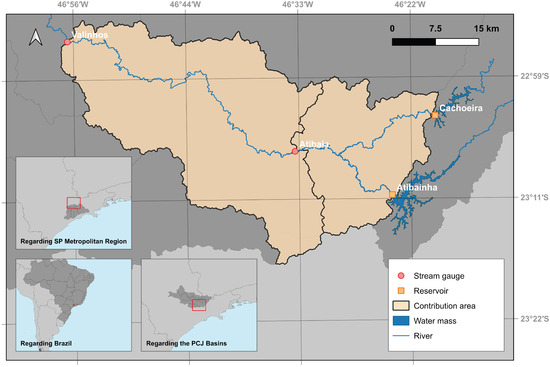
Figure 1.
Location of the study area.
2.2. Hydrological Models
To better understand how the final model was structured, which combines a rainfall–runoff module with a river routing module, the flowcharts (see Figure 2) relate each implemented process and its execution order. The steps marked in blue represent essential modeling procedures examined in future sections. Those in orange correspond to outputs from previous processes, while those in gray represent known data.
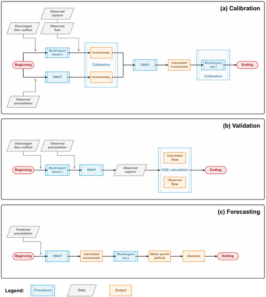
Figure 2.
Research flowchart.
In Figure 2, research flowcharts are divided into (a) calibration, (b) validation, and (c) prediction stages. In (a), to identify the required discharges to meet the minimum specified flows at each gauge downstream, the model initially records the past releases from each dam (based on a predefined historical series of observed outflows recorded for Atibainha and Cachoeira reservoirs) and translates these hydrographs to the first encountered point using a method for river routing called the Muskingum model (towards downstream) [31,32]. Based on observed flows at the first stream gauge and water withdrawals for supply and consumption, a separation of components is performed to calibrate the parameters applied in the routing model jointly with the variables necessary for the rainfall–runoff conversion, which is calculated by a model called SMAP [33]. The technique employed to calibrate the increments of each process (routing and rainfall–runoff) corresponds to a differential evolution algorithm. The same procedure is then repeated between the first and second gauges; now, the observed flows registered in the first point are translated to the second point, whereby a new separation and calibration of variables is performed using the calculated flow increments via Muskingum and SMAP. With the hydrologic model properly adjusted, it is then necessary to adapt the backwater parameters for application in the reverse Muskingum routing scheme (which moves upstream, from outlet to inlet hydrographs).
In summary, the calibration is performed in the incremental basins, between the reservoirs and the first stream gauge (Atibaia sub-basin) and between the first and second stream gauge (Valinhos sub-basin). Thus, the parameters of the rainfall–runoff model and the parameters of the hydrological routing are defined for specific river sections. Subsequently, in (b), the validation is carried out by using the calibrated parameters to calculate the streamflow at each stream gauge. Using the discharges, routing is performed to the points, the runoff contribution from rainfall–runoff conversion is added, and water withdrawals along the river are subtracted. The calculated flows between sections are then compared with the measured flows for the same period.
Finally, in (c), a 7-day series of meteorological forecasts is used to feed the rainfall–runoff module, backtracking to the source reservoirs, and comparing the hydrographs obtained with the demands specified by the water use permits. The release required to ensure downstream water security corresponds to the largest positive difference between the forecasted future flow and the daily minimum flow. To complement the flowcharts and visually represent the processes, Figure 3 shows an explanatory illustration.
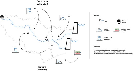
Figure 3.
Model diagram.
At the top, during calibration, we call the discharges from Atibainha and Cachoeira reservoirs, which are converted by traditional river routing into incremental flows called (after separating portions). Concurrently, observed precipitations called are transformed into incremental flows . Together, and are used to calibrate the rainfall–runoff and routing modules. At the bottom, for forecasting, we call the predicted precipitations, which are transformed into forecast flows . The estimated flows are retroceded to the reservoirs by reverse routing. When compared to the minimum allocations, the ordinates above (green range) indicate minimum discharges , while the ordinates below (red range) indicate dam discharges equal to the calculated deficits.
It is important to highlight that the need to apply the reverse routing technique mitigates the use of more complex equations for optimizing reservoir discharges. Instead of formulating more intricate objective functions without guarantees of achieving desirable optima, tracing the outflows from sub-basin outlets back to the reservoirs is more intuitive and straightforward. This approach leads to more accurate results and represents an innovative contribution to the study, as it has been scarcely explored in the technical literature.
2.2.1. SMAP Model
Hydrologic models consist of a composition of algorithms that describe processes inherent to the hydrological cycle, such as spatial distribution of precipitation, losses due to interception or evaporation, infiltration flow, and surface runoff. In this research line, Soil Moisture Accounting Procedure (SMAP) is a conceptual rainfall–runoff lumped model proposed by [33] with monthly, daily, or hourly discretization levels. One of the key factors supporting the use of the SMAP model in Brazil is its extensive application in the Brazilian electric sector, particularly by the National System Operator (ONS), for power planning studies integrated with reservoir operation [34].
In its daily version, the model interprets storage and flows in three linear reservoirs (see Figure 4):
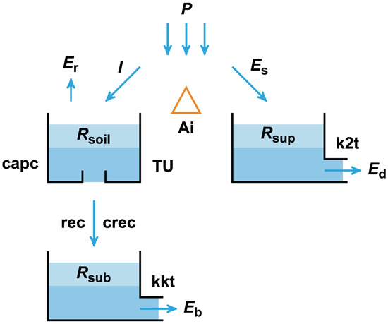
Figure 4.
SMAP model.
In a daily step, the following relationships apply:
in which corresponds to a reservoir associated with the soil in its unsaturated zone, to the one in the saturated zone, and to a surface reservoir. , , and refer to surface and direct runoff, and base flow, respectively, while represents actual evapotranspiration, P is precipitation, and is groundwater recharge (all units given in millimeters).
To apply the model, series of observed daily rainfall, streamflow, and potential evapotranspiration () are used, all of which are necessary to calibrate six parameters: saturation capacity (SAT) (mm), recession constant for (days), recharge capacity (%), initial abstraction (mm), field capacity (%), and recession constant for (days). By providing values for the initial moisture content () as well as the initial base flow (), and knowing the drainage area () of interest, the following steps are initially taken:
Next, for each day with rainfall, five calculations are carried out:
- (1)
- If , then . Otherwise, .
- (2)
- If , then . Otherwise,
- (3)
- If , then . Otherwise, .
- (4)
- (5)
After evaluating the reservoirs using the three initial relationships, we calculate
Despite the large number of studies that apply alternative rainfall–runoff conversion models, such as those distributed in the HEC or SWAT software [35,36], the choice of the SMAP model over alternatives such as HEC-HMS or SWAT is justified by its sound representation of the hydrological cycle, ease of implementation, and low computational cost. In studies such as [37], SMAP-based streamflow forecasts yielded notably lower errors than SWAT for a Brazilian watershed, for example. Although SMAP is more widely known and used in Brazilian studies, its benefits are also applicable in other regions with comparable hydrological characteristics. Not encapsulated within a distribution, the model consists of an algorithm that can be replicated in any programming language. In this study, the rainfall–runoff module and hydrological routing, along with calibration and overall plotting, were entirely coded in Python (version 3.12.3), utilizing data processing libraries such as matplotlib, numpy, pandas, and scipy. Furthermore, the relatively small number of variables to be calibrated encouraged the choice of this model over other solutions. The use of SMAP is also supported by analogous studies, such as [5,34,38].
2.2.2. Nonlinear Muskingum Model
An example of a flood routing and attenuation model in hydraulic channels is the Muskingum method, developed by [32]. Given the hydrological continuity equation,
(where I represents an inflow hydrograph, O an outflow hydrograph, and S the storage within the channel), [39] emphasizes that the numerical relationship between weighted flows and river storage is nonlinear. In fact, in practical problems, one deals with hydrographs with n flow peaks, notably different from those studied in texts recommending the first-order linear Muskingum method. Therefore, the more appropriate Muskingum storage model for the research, as presented by [31], although less traditional, corresponds to the relationship
In it, K represents the mean travel time of a flood wave between upstream and downstream sections, while X corresponds to a weighting factor or damping factor, and m is a nonzero real exponent.
To obtain an outflow hydrograph from an inflow hydrograph, and given the three variables K, X, and m that compose the model, it is necessary to use a numerical approach that approximates the differential equation of continuity. One possibility in this case is to use the fourth-order Runge–Kutta method, or FORK [39]. Initially, values are assumed for K, X, and m, and then a storage is calculated based on an imposed initial condition (, for example). Then, to obtain the subsequent storage , the derivative is calculated using an estimated slope with four parameters:
Once the four coefficients are calculated, we have that
To complete the time step and obtain the desired downstream ordinate, we perform
Using an input hydrograph with n ordinates, the method is applied from to .
2.2.3. Upstream Routing
A direct way to calculate the required discharges to meet downstream water demands after knowing the incremental contribution of future rainfall is to identify if the predicted flow with precipitation meets the minimum required discharge at a control section. If not, only the excess volume of water is released for supply. The hydrograph obtained from the weather forecasts is computable and known, as well as the minimum average daily values for each point of interest. Thus, the outlined problem involves determining which upstream discharge hydrograph, from the reservoirs, will result in the downstream hydrograph after leaving the dams and flowing through the watercourse (to meet water deficits, if any). In other words, from the output hydrograph, the goal is to obtain the input hydrograph through reverse routing. Despite being less common than the conventional upstream-to-downstream routing, many authors, such as [40,41,42], have analyzed such a situation in past studies. However, [43] warns that simply inverting the calculation between I and O does not constitute a well-defined problem according to the Muskingum method, and, consequently, computational rounding errors or input data errors are expected to be quickly amplified and propagated between numerical iterations. For the nonlinear first-order case, [41] follows [39] and proposes the FORK algorithm as a technique for reverse routing. According to the author, after obtaining values for , , and , the calculation starts by determining a storage based on a certain initial condition, such as . Subsequently, four parameters are necessary to estimate the rate :
With them, the previous storage is determined by
To complete the time step and obtain the desired upstream ordinate, we perform
From an output hydrograph with n ordinates, the method is applied from to 1.
2.3. Calibration and Validation of Hydrological Models
The prediction of future flows from rainfall events is essential for a dam operator, who manages the reservoirs based on short-term weather estimates. To obtain reliable flow values in a hydrological model, it is necessary to calibrate the physical variables to values consistent with the regional dynamics of the study area. According to [33], the SMAP model includes six free parameters; however, the author suggests fixing three of them as constants and automatically calibrating the remaining three. The initial abstraction and field capacity can be directly measured with previous knowledge of land use (vegetation cover) and soil type. The recession constant is less sensitive to calibration objective functions, allowing for a fixed manual adjustment.
To assess the parameters of saturation capacity, recession constant for surface runoff, and recharge capacity, there are known lower and upper limits: mm, days, and %. With these boundary conditions, the challenge is to determine values such that the final flows calculated with the model are sufficiently consistent with values determined by hydrological routing, minimizing the differences between both incremental series. In addition to the set of SMAP parameters, two additional variables should be considered and calibrated: (i) the ones responsible for initiating the simulation (initial moisture content and base flow ), and (ii) the Muskingum variables K, X, and m, and their variants for the upstream type. Therefore, two additional intervals were included for SMAP: and m3s−1. For the Muskingum parameters, whether for the traditional nonlinear model or for the inverse, the following ranges were considered: days, , and .
The objective function considered in the study is the Nash–Sutcliffe coefficient:
The procedure established to simulate the described problem and ensure the calculation of future dam outflows involves selecting a historical series of rainfall, streamflows, discharges, and water withdrawals, and calibrating the SMAP and Muskingum variables for each incremental basin and reach of the watercourse (totaling three hydrological terms for Atibaia and its basin, plus three for Valinhos, in addition to six routing terms for each river stretch: from Atibainha to Atibaia, from Cachoeira to Atibaia, and from Atibaia to Valinhos). This process corresponds to the “Calibration” flowchart in Figure 2. Then, for each discharge decision day, to be calculated via meteorological forecast, a unique determination of only two initial data points is made: the terms and , while all the other variables are fixed with the previously calibrated values.
The validation of the calibrated parameters was performed through direct comparisons between the flow balance at the stream gauges and the actual flow measurements recorded during the period. After routing the discharges, adding rainfall contributions, and subtracting water withdrawals along the river course (due to industrial permits or public supply usage), the final verification was conducted using the Kling–Gupta efficiency coefficient, given by the following:
where r is the Pearson correlation coefficient, is the standard deviation, and is the mean.
2.4. Data
The data collected for simulating discharges to the PCJ Basins consists essentially of two types: observed and predicted data. Observed water withdrawals between the reservoirs and control points were obtained from DAEE, São Paulo’s Department of Water Resources, available at [44]. A total of 2193 days, from 1 January 2015 to 1 January 2021, were used for calibration (approximately 6 years), and 1356 days, from 2 January 2021 to 18 September 2024, were used for validation and prediction (approximately 4 years). Regarding the observed discharges at Atibainha and Cachoeira, the observed time series were derived from discharge records computed using each dam’s spillway rating equations [45]. Daily precipitation and streamflow at Atibaia and Valinhos were sampled from a Decision Support System (DSS) of the Basic Sanitation Company of the State of São Paulo (Sabesp), also available in [45]. The streamflow data comes from local streamflow gauging stations as the points are also stations managed by DAEE, measured via stage–=discharge rating curves that convert river stage (water levels) to discharge. In turn, the observed precipitation is estimated using a meteorological radar and provided by the Flood Alert System of São Paulo (SAISP) [46]. The values collected are recorded for each incremental basin. Finally, the predicted precipitation data was obtained from the Paraná Environmental Monitoring and Technology System (SIMEPAR), a Brazilian institution that utilizes the WRF (Weather Research & Forecasting) meteorological model for forecasting precipitation [47]. All datasets were also compiled into a single public repository, available in [48].
Although the model calibrates a set of variables before executing the forecast scenario, certain parameters for use with the SMAP module are kept fixed throughout its simulation. For Atibaia, we have km2. For Valinhos, km2. Both used mm, , and days.
Meteorological Forecasts and Their Structure
As aforementioned, the coupled model was structured to receive a set of seven meteorological forecasts at each step, used to convert into future streamflow values to be evaluated for compliance with local water resource permits. The dam release decision routines follow the following pattern: at each iteration, 30 days of observed data are used as modules inputs, as even after the 6-year calibration that determines the SMAP variables and Muskingum routing (both downstream and upstream), it is still necessary to initiate the rainfall–runoff algorithm with an initial soil moisture content () and a base flow (). In other words, a quick calibration is performed using 1 month of observed data. After this, at the end of each 30-day series, a vector of 7 days of future rainfall is added. With the set of days and the determined initial parameters, the prediction and backtracking of hydrographs to the source reservoirs are simulated. Note that at each step, the 7-day forecast vectors are renewed, as the data for each iteration is different and not repeated. As the objective of this article is to also vary the input forecasts, a scenario was prepared in which the rainfall predictions are observed rainfall measurements from the rain gauge stations. Thus, a situation was constructed where the 7-day future vectors are populated with observed rainfall data from each sub-basin. In this new approach, the dataset is entirely based on observed data and is simply shifted forward by one day at each iteration (therefore, the ‘forecast’ datasets include repeated data between steps). For more details, see Figure 5.
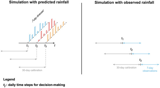
Figure 5.
Forecast data structure in each scenario.
3. Results
Table 1 and Table 2, respectively, show the parameters obtained for the hydrologic model and for traditional and inverse nonlinear routing methods.

Table 1.
SMAP parameters calibrated with observed series (SAT is the soil saturation capacity, is the fraction of days for surface runoff recession, is the recharge of the groundwater reservoir, is the initial soil moisture content, and is the initial base flow).
Table 2.
Muskingum parameters calibrated with observed series (K in days is the travel time of the flood wave, X is the peak attenuation factor of the hydrograph, and m is the nonlinear constant of the model, both dimensionless).
Using a three-parameter subset for calibration (out of the six parameters of the rainfal–runoff model), we found that the most influential free parameter for the final incremental hydrographs is the soil saturation capacity. Higher values reflect the model’s attempt to better reproduce the observed peaks in natural flow and are consistent with the study region, which still exhibits limited land-use/land-cover disturbance [49]. As in similar research [34,50,51], it is not practical to directly compare parameter values across studies, as each work calibrates the hydrologic information to its own basins. Even so, the saturation capacity and the surface runoff recession time tend to be comparable to those reported by [51] for a basin also located in southeastern Brazil, and the recharge capacity is of the same order of magnitude as that inferred by [50] for a set of basins that are hydrologically similar to those analyzed here.
Regarding the Muskingum parameters governing nonlinearity, flood-wave translation, and peak attenuation, we observe strong internal consistency for the Valinhos incremental basin (between the Atibaia and Valinhos gauges). For the Atibaia incremental basin (between the Atibaia gauge and each reservoir), however, a complicating factor is the natural confluence of tributaries; under reverse routing (towards upstream), it is not possible to precisely apportion the contribution of each river segment. Consequently, the optimizer sought a global optimum for the objective function at the expense of physical coherence in that reach: upstream travel times are approximately two days longer than downstream times for the same segments. Part of this behavior reflects the joint, simultaneous calibration of the hydrologic components, whose objective function reduces errors in incrementally computed flows. This solution was adopted to overcome the lack of direct records of rainfall-derived streamflow in the study area.
A more suitable and visual way to understand the calibration results is to plot the incremental flows obtained via SMAP and Muskingum for Atibaia and Valinhos, using the data provided in the tables. For the predicted rainfall scenario, see Figure 6 and Figure 7.
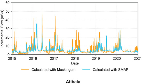
Figure 6.
Comparison of incremental hydrographs during the calibration round for Atibaia.
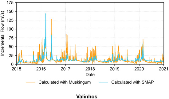
Figure 7.
Comparison of incremental hydrographs during the calibration round for Valinhos.
The calibration of parameters conducted over the 6-year dataset indicated Nash–Sutcliffe coefficient values of 0.541 and 0.581 for Atibaia and Valinhos, respectively, according to Figure 6 and Figure 7. It is possible to observe upper flow limits of about 50 m3s−1 at Atibaia and nearly 150 m3s−1 at Valinhos, with differences directly related to the total drainage area at each point. Because the incremental series derived from routing are more strongly influenced by observed data, whereas those obtained via SMAP depend mostly on the calibrated parameters, the orange peaks (Muskingum) tend to be sharper and more frequent than the blue ones (SMAP). Validation of calibrated parameters over a four-year period (see Figure 8 and Figure 9) yielded a Kling–Gupta efficiency (KGE) of approximately 0.38.
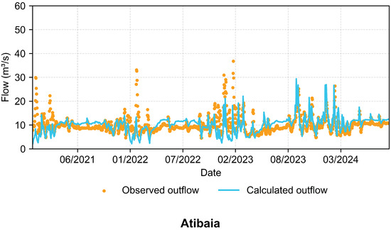
Figure 8.
Validation flow rates at the Atibaia stream gauge.
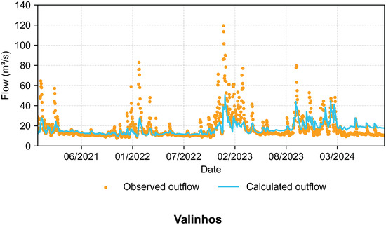
Figure 9.
Validation flow rates at the Valinhos stream gauge.
Whereas Figure 8 indicates a stronger correspondence between observed and simulated flows, Figure 9 for Valinhos shows greater divergence and underperformance. Peak discharges during the wet periods of 2022 and 2023 were not adequately reproduced, which depresses the KGE value.
To validate the model and its accuracy as a decision support tool, it is necessary to first present and compare the numerically calculated and actual discharge values and additionally confirm whether the modeled dam outflows were effective in ensuring equal or higher flows than the minimum required for each gauge. Figure 10 shows discharges with forecast data:
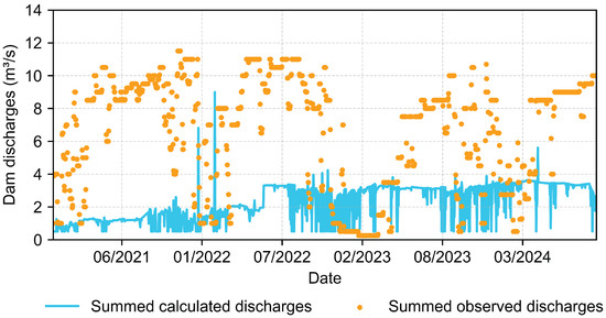
Figure 10.
Calculated dam discharges with meteorological forecasts in relation to actual discharges.
As shown in Figure 10, the model reduces the decision discharges to values lower than those observed. This nature is inherent to the coupled model and the way it operates the reservoirs. In real situations, compliance with water permits must be reconciled with the maneuvering times of hydraulic gates and with the flood propagation time to downstream sections. Although the model considers the second condition, it does not maintain constant maneuvers. Therefore, the discharges oscillate more frequently. Mathematically, the simulation aims to comply with the rules imposed as boundary conditions. When the highest average daily minimum is met in a rainfall–runoff step, the reservoirs release the minimum amount prescribed in the permit of 0.25 m3s−1. If the given day indicates the need for releasing a greater water volume, the model responds with automatic discharges that can jump from 0.25 to 1.50 m3s−1, for example, or higher.
For the Atibaia stream gauge, with its minimum average daily requirement of 2 m3s−1, the following results ensue (see Figure 11).
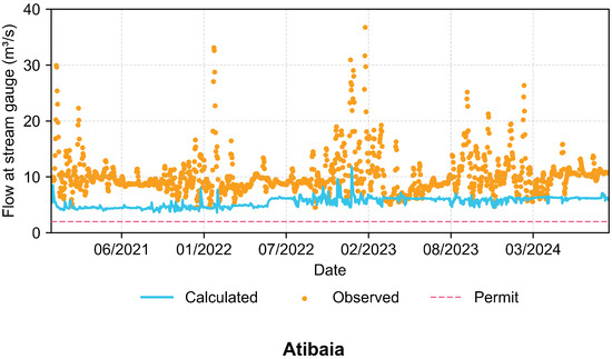
Figure 11.
Flows verified at the Atibaia point after discharge decisions with forecasts.
In contrast, Valinhos stream gauge results, with its daily minimum of 10 m3s−1, are plotted in Figure 12.
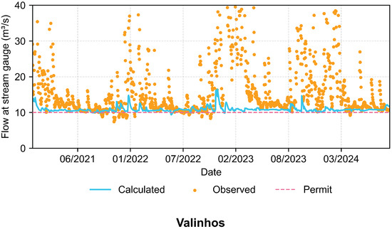
Figure 12.
Flows verified at the Valinhos point after discharge decisions with forecasts.
In the simulated gauge sections, as seen in Figure 11 and Figure 12, it is possible to observe that the hydrographs of the calculated flows align with the minimum expected flows at each point. As the calculated hydrographs in blue result from the translated discharged flow to the section plus the rainfall–runoff component derived from predicted rainfall minus water withdrawals, corresponding flow peaks can be observed during wet periods, as expected. Conversely, during drier conditions, the discharge is responsible for meeting the minimum flow requirements. Given that the calculated curve does not cross the dashed permitted line on any simulation day in Atibaia, the model ensured at least the minimum required flow throughout all the simulated days. In Valinhos, the flow requirement was unmet for 25 days over 4 years, with a minimum flow of 9.4 m3s−1. Despite a lower total compliance of 98%, the minimum water guarantee is still practically ensured at the simulated point.
To avoid redundancy, one way to add the results in the observed rainfall scenario and contrast the simulations with forecasts, observations, and real data over the 4-year period is to calculate the area underneath each generated hydrograph and, thus, assess the accumulated discharged volumes (see Figure 13).
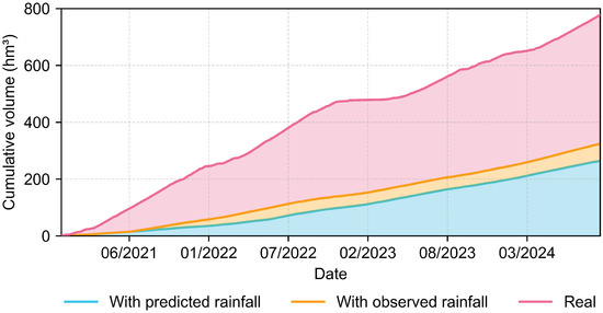
Figure 13.
Relationships between the different discharges for each scenario.
Another way to visualize the distributions of the decisions is through boxplots, as shown in Figure 14.
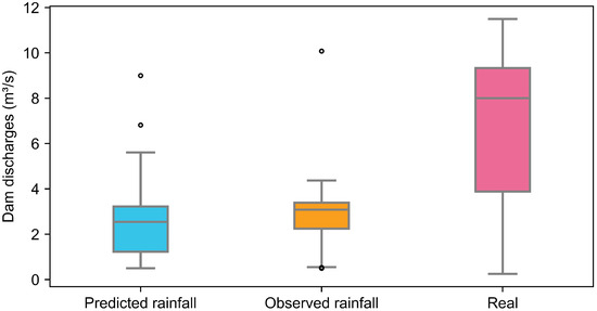
Figure 14.
Discharge boxplot distributions.
As the model focuses solely on meeting the condition of the minimum average daily discharge in a hypothetically critical situation in which the Cantareira System is operated, the discharged volumes downstream with meteorological predictions amounted to approximately 263 hm3 (billions of liters) over the course of four years of simulation, compared to 770 hm3 in actual data for the same period (see Figure 13). The specific objective of introducing an optimal forecast scenario, in which the weather forecast matches the observed rainfall, was also successfully achieved, indicating accumulated volumes of 323 hm3. Despite the expectation that optimal forecasts would lead to better decisions by the model, the greater water savings in the predicted rainfall scenario compared to the observed rainfall scenario may be attributed to the initialization conditions of the models in each simulated case.
4. Discussion
Within the broader context of optimal reservoir operation, the present study falls under the “Real-Time Optimization” category, described by [52] as optimization over moving horizons. Our use of hydrological routing to estimate short-term discharges differs from similar Brazilian studies, such as [53,54], which rely on stochastic or machine-learning-based optimization. Relying on physical hydrological concepts facilitates implementation and describes hydrological cycle and channel dynamics in a parsimonious way. Because of that, the same methodology can be applied elsewhere, provided that adequate climate and hydrological monitoring networks are available to supply data for calibration, validation, and forecasting.
Overall, the results for cumulative released volume (Figure 13) and the distribution of releases (Figure 14) show that the coupled rainfall–runoff and routing model can substantially reduce water use in regional reservoir operations in the study area. Model water releases could be up to 66% lower in comparison to the observed scenario without optimization. A similar optimization model by [54] showed that improved hydrometeorological data and information applied in hydropower production systems allows for better water storage management across time, with increased energy production and value. Despite these promising outcomes, the difference in simulated and observed releases shown in Figure 10 disregard the operational difficulties in controlling discharge with high precision. Frequent oscillations from the optimal simulation are not fully consistent with actual reservoir operating rules, observed in historical discharge data. For future work, we suggest integrating a multi-objective optimization framework that both enforces public-supply policies and smooths operational releases from the dams.
The optimized simulation meets the minimum flows required at Atibaia throughout the entire period, whereas at Valinhos there were 25 days of noncompliance over four years, with a minimum flow of 9.4 m3 s−1 (Figure 11 and Figure 12). The slightly lower overall compliance rate (98%) stems from numerical precision errors in the routing approach, which propagate from downstream to upstream and subsequently from upstream to downstream. As noted by [43], reverse routing is ill-posed and is, thus, susceptible to inherent numerical oscillations, which corroborates this limitation.
The model’s low sensitivity to peak flows, as indicated by modest NSE and KGE values, are consistent with the findings of [49], which limits its suitability for flood-related applications. However, its reliable simulation of recessions supports its use in drought mitigation and reservoir management. Comparing Figure 6 and Figure 7, the markedly different peak magnitudes arise from the incremental rainfall contribution across the sub-basins associated with each control point. Because Valinhos drains an area more than twice the size of Atibaia, the rainfall–runoff component exerts a stronger influence on the calibrated hydrograph there. The same pattern is observed during validation (Figure 8 and Figure 9), where peak underestimation at Valinhos is more evident, consistent with the SMAP model’s behavior.
5. Conclusions
This study highlights the potential of hydrological modeling, when integrated with meteorological forecasts, to optimize reservoir operations in the Cantareira System and PCJ Basins. The coupled model demonstrated its ability to reduce water releases by up to 66% in forecast-based scenarios compared to actual operational data, all while maintaining compliance with minimum flow requirements at stream gauges. These findings emphasize the effectiveness of predictive tools in balancing environmental obligations with legal constraints, thereby supporting enhanced decision-making processes to ensure water security. Moreover, this novel forecasting application in the Cantareira/PCJ context can streamline near-term operations, yield water-saving benefits, and maintain regulatory compliance, despite the simplifying assumptions of the modeling approach. Overall, the findings represent a foundation for multi-objective optimization frameworks that could drastically improve reservoir efficiency.
The use of short-term forecasts with indications of water savings reiterates the utility of the methodology as a tool for management support, resilience to climatic extremes, and operational flexibility to meet complex and conflicting water uses. By drawing on established hydrological techniques that remain underexplored in Brazilian studies—such as nonlinear and reverse Muskingum routing—valuable insights are offered to contribute to the optimization of reservoir operations in both national and international contexts. This methodological combination (rainfall–runoff plus forward and reverse routing) represents an innovation of practical relevance for operators who require simple, explainable tools that can be embedded into routine decision workflows.
Despite its promising outcomes, the model faced challenges in addressing the mitigation of sudden discharge fluctuations (which do not reflect the reality of dam gate operations), or meeting the requirement of minimum moving average demands over 15 days. As such, the model should be subjected to multi-objective optimization that reduces the number of operations and proposes more consistent discharge hydrographs.
The methodology developed in this work provides a robust framework that can be adapted to similar reservoir systems worldwide, particularly in regions grappling with water scarcity and complex water management structures. The integration of predictive analytics and computational techniques provides valuable insights for addressing challenges in fields such as drought risk reduction and climate resilience planning. Researchers and practitioners in these domains can build upon these findings to develop customized solutions that enhance the efficiency and sustainability of water resource allocation, contributing to broader resilience and adaptability in managing environmental challenges.
Author Contributions
R.F.P.: Conceptualization, methodology, software, investigation, writing—original draft. J.R.B.T.: Conceptualization, methodology, data curation, writing—review and editing. D.H.H.: Methodology, software, investigation, writing—review and editing. V.L.G.R.: Writing—review and editing. J.I.B.: Conceptualization, methodology, validation, resources, supervision, funding acquisition. All authors have read and agreed to the published version of the manuscript.
Funding
The research presented herein was funded through a graduate grant provided by Fundação Centro Tecnológico de Hidráulica (FCTH), a private nonprofit entity collaborating with the Polytechnic School of the University of São Paulo, where the researchers are affiliated.
Data Availability Statement
The data underlying this manuscript is available at HydroShare under https://doi.org/10.4211/hs.609b5b375a16404f9c4d14417264a7fb. The code written in Python is hosted at GitHub under https://github.com/Raphael-18/projeto-de-pesquisa (accessed on 8 October 2025).
Acknowledgments
The authors would like to thank FCTH for the research funding grant and also the Graduate Program in Civil Engineering at the Polytechnic School of the Universidade de São Paulo and Coordenação de Aperfeiçoamento de Pessoal de Nível Superior – Brasil (CAPES).
Conflicts of Interest
The authors declare no conflicts of interest.
References
- Sone, J.S.; Araujo, T.F.; Gesualdo, G.C.; Ballarin, A.S.; Carvalho, G.A.; Oliveira, P.T.S.; Wendland, E.C. Water Security in an Uncertain Future: Contrasting Realities from an Availability-Demand Perspective. Water Resour. Manag. 2022, 36, 2571–2587. [Google Scholar] [CrossRef]
- Mekonnen, M.M.; Hoekstra, A.Y. Four billion people facing severe water scarcity. Sci. Adv. 2016, 2, e1500323. [Google Scholar] [CrossRef] [PubMed]
- Van Vliet, M.T.H.; Jones, E.R.; Flörke, M.; Franssen, W.H.P.; Hanasaki, N.; Wada, Y.; Yearsley, J.R. Global water scarcity including surface water quality and expansions of clean water technologies. Environ. Res. Lett. 2021, 16, 024020. [Google Scholar] [CrossRef]
- Marques, A.C.; Veras, C.E.; Rodriguez, D.A. Assessment of water policies contributions for sustainable water resources management under climate change scenarios. J. Hydrol. 2022, 608, 127690. [Google Scholar] [CrossRef]
- Michelan, M.G.; Menegaz, M.N.; Gonçalves, F.A.; Menezes, P.H.B.J.; Tiezzi, R.O. Estimating the impact of climate change on water levels in a data-poor river basin in southeastern Brazil. Water Policy 2021, 23, 1284–1302. [Google Scholar] [CrossRef]
- Inomata, H.; Kawasaki, M.; Kudo, S. Quantification of the Risks on Dam Preliminary Release Based on Ensemble Rainfall Forecasts and Determination of Operation. J. Disaster Res. 2018, 13, 637–649. [Google Scholar] [CrossRef]
- Yaghmaei, H.; Sadeghi, S.H.; Moradi, H.; Gholamalifard, M. Effect of Dam operation on monthly and annual trends of flow discharge in the Qom Rood Watershed, Iran. J. Hydrol. 2018, 557, 254–264. [Google Scholar] [CrossRef]
- Manca, R.S.; Falconi, S.M.; Zuffo, A.C.; Dalfré Filho, J.G. Contributions to increase the availability of water supply in regions of water shortage: The case study of São Paulo, Brazil. In The Sustainable City IX. WIT Transactions on Ecology and The Environment; WIT Press: Southampton, UK, 2014. [Google Scholar] [CrossRef]
- Zuffo, A.C.; Duarte, S.N.; Jacomazzi, M.A.; Cucio, M.S.; Galbetti, M.V. The Cantareira System, the Largest South American Water Supply System: Management History, Water Crisis, and Learning. Hydrology 2023, 10, 132. [Google Scholar] [CrossRef]
- Tercini, J.R.B.; Perez, R.F.; Schardong, A.; Bonnecarrère, J.I.G. Potential impact of climate change analysis on the management of water resources under stressed quantity and quality scenarios. Water 2021, 13, 2984. [Google Scholar] [CrossRef]
- Coelho, C.A.S.; de Oliveira, C.P.; Ambrizzi, T.; Reboita, M.S.; Carpenedeo, C.B.; Campos, J.L.P.S.; Tomaziello, A.C.N.; Pampuch, L.A.; de Souza Custódio, M.; Dutra, L.M.M.; et al. The 2014 southeast Brazil austral summer drought: Regional scale mechanisms and teleconnections. Clim. Dyn. 2016, 46, 3737–3752. [Google Scholar] [CrossRef]
- Domingues, L.M.; de Abreu, R.C.; da Rocha, H.R. Hydrologic Impact of Climate Change in the Jaguari River in the Cantareira Reservoir System. Water 2022, 14, 1286. [Google Scholar] [CrossRef]
- Gozzo, L.F.; Drumond, A.; Pampuch, L.A.; Ambrizzi, T.; Crespo, N.M.; Reboita, M.S.; Bier, A.A.; Carpenedo, C.B.; Bueno, P.G.; Pinheiro, H.R.; et al. Intraseasonal Drivers of the 2018 Drought Over São Paulo, Brazil. Front. Clim. 2022, 4, 852824. [Google Scholar] [CrossRef]
- Otto, F.E.L.; Haustein, K.; Uhe, P.; Coelho, C.A.S.; Aravequia, J.A.; Almeida, W.; King, A.; de Perez, E.C.; Wada, Y.; van Oldenborgh, G.J.; et al. Factors Other Than Climate Change, Main Drivers of 2014/15 Water Shortage in Southeast Brazil. Bull. Am. Meteorol. Soc. 2015, 96, S35–S40. [Google Scholar] [CrossRef][Green Version]
- Cho, S.J.; Klemz, C.; Barreto, S.; Raepple, J.; Bracale, H.; Acosta, E.A.; Rogéliz-Prada, C.A.; Ciasca, B.S. Collaborative Watershed Modeling as Stakeholder Engagement Tool for Science-Based Water Policy Assessment in São Paulo, Brazil. Water 2023, 15, 401. [Google Scholar] [CrossRef]
- Schardong, A.; Simonovic, S.P.; Vasan, A. Multiobjective Evolutionary Approach to Optimal Reservoir Operation. J. Comput. Civ. Eng. 2013, 27, 139–147. [Google Scholar] [CrossRef]
- Tundisi, J.G.; Matsumura-Tundisi, T. Integration of research and management in optimizing multiple uses of reservoirs: The experience in South America and Brazilian case studies. Hydrobiologia 2003, 500, 231–242. [Google Scholar] [CrossRef]
- Lopes, T.R.; Folegatti, M.V.; Duarte, S.N.; Zolin, C.A.; Fraga, L.S., Jr.; Moura, L.B.; Oliveira, R.K.; Santos, O.N.A. Hydrological modeling for the Piracicaba River basin to support water management and ecosystem services. J. South Am. Earth Sci. 2020, 103, 102752. [Google Scholar] [CrossRef]
- Méllo Júnior, A.V.; Olivos, L.M.O.; Billerbeck, C.; Marcellini, S.S.; Vichete, W.D.; Pasetti, D.M.; da Silva, L.M.; dos Santos Soeares, G.A.; Tercini, J.R.B. Rainfall Runoff Balance Enhanced Model Applied to Tropical Hydrology. Water 2022, 14, 1958. [Google Scholar] [CrossRef]
- Wang, Y.; Karimi, H.A. Impact of spatial distribution information of rainfall in runoff simulation using deep learning method. Hydrol. Earth Syst. Sci. 2022, 26, 2387–2403. [Google Scholar] [CrossRef]
- Fontes Santana, R.; Celeste, A.B. Stochastic reservoir operation with data-driven modeling and inflow forecasting. J. Appl. Water Eng. Res. 2022, 10, 212–223. [Google Scholar] [CrossRef]
- Lopes, M.S.; Tercini, J.R.B.; De Santi, A.D.; Pedrozo, D.B.; Garcia, J.I.B.; Gonzalez, V.A.R.; Léo, E.C. Decision support system applied to water resources management: PCJ Basins case study. Rev. Gestão Ambient. Sustentabilidade 2021, 10, e19876. [Google Scholar] [CrossRef]
- Giuliani, M.; Lamontagne, J.R.; Reed, P.M.; Castelletti, A. A State-of-the-Art Review of Optimal Reservoir Control for Managing Conflicting Demands in a Changing World. Water Resour. Res. 2021, 57, e2021WR029927. [Google Scholar] [CrossRef]
- Kim, G.J.; Kim, Y.-O. How Does the Coupling of Real-World Policies with Optimization Models Expand the Practicality of Solutions in Reservoir Operation Problems? Water Resour. Manag. 2021, 35, 3121–3137. [Google Scholar] [CrossRef]
- Souza, J.D.S.; Cirilo, J.A.; Bezerra, S.T.M.; Oliveira, G.A.D.; Freire, G.D.; Coutinho, A.P.; Cabral, J.J.D.S.P. Decision Support System for the Integrated Management of Multiple Supply Systems in the Brazilian Semiarid Region. Water 2023, 15, 223. [Google Scholar] [CrossRef]
- Almagro, A.; Oliveira, P.T.S.; Ballarin, A.S. SSP-CABra—Streamflow Scenarios Projections for Brazilian Catchments. Geosci. Data J. 2025, 12, e70029. [Google Scholar] [CrossRef]
- Ballarin, A.S.; Godoy, M.R.V.; Zaerpour, M.; Abdelmoaty, H.M.; Hatami, S.; Gavasso-Rita, Y.L.; Wendland, E.; Papalexiou, S.M. Drought intensification in Brazilian catchments: Implications for water and land management. Environ. Res. Lett. 2024, 19, 054030. [Google Scholar] [CrossRef]
- González-Zurita, J.; Oswald-Spring, Ú. Modeling water availability under climate change scenarios: A systemic approach in the metropolitan area in Morelos, México. Front. Water 2024, 6, 1466380. [Google Scholar] [CrossRef]
- Tercini, J.R.B.; Méllo Júnior, A.V. Impact of hydroclimatic changes on the operation of water resources systems: A case study of the Cantareira Water Production System. Rev. Bras. Recur. Hídricos 2024, 29, e19. [Google Scholar] [CrossRef]
- Agência Nacional de Águas e Saneamento Básico (ANA). Resolução Conjunta ANA/DAEE N° 925, de 29 de Maio de 2017; Brasília. 2017. Available online: https://www.gov.br/ana/pt-br/legislacao/resolucoes/resolucoes-regulatorias/2017/925 (accessed on 25 September 2025).
- Chow, V.T. Open Channel Hydraulics; McGraw-Hill: New York, NY, USA, 1959. [Google Scholar]
- McCarthy, G.T. Unit hydrograph and flood routing. In Proc. Conf. North Atl. Div. 1938, 1938, 608–609. [Google Scholar]
- Lopes, J.E.G.; Braga, B.P.F.; Conejo, J.G.L. SMAP: A simplified hydrologic model. In Applied Modeling in Catchment Hydrology; W.R.P: Littleton, CO, USA, 1982; pp. 167–176. [Google Scholar]
- Maciel, G.M.; Cabral, V.A.; Marcato, A.L.M.; Junior, I.C.S.; Honorio, L.D.M. Daily Water Flow Forecasting via Coupling Between SMAP and Deep Learning. IEEE Access 2020, 8, 204660–204675. [Google Scholar] [CrossRef]
- Ferraz, L.L.; Santana, G.M.; de Sousa, L.F.; da Silva Amorim, J.; Santos, C.A.S.; de Jesus, R.M. Databases and Applications of the Soil and Water Assessment Tool (SWAT) Model in Brazilian River Basins: A Review. Environ. Model. Assess. 2024, 30, 349–367. [Google Scholar] [CrossRef]
- Moraes, T.C.; dos Santos, V.J.; Calijuri, M.L.; Torres, F.T.P. Effects on runoff caused by changes in land cover in a Brazilian southeast basin: Evaluation by HEC-HMS and HEC-GEOHMS. Environ. Earth Sci. 2018, 77, 250. [Google Scholar] [CrossRef]
- Chen, M.; Cataldi, M.; Francisco, C.N. Application of hydrological modeling related to the 2011 disaster in the mountainous region of Rio de Janeiro, Brazil. Climate 2023, 11, 55. [Google Scholar] [CrossRef]
- Neves, G.L.; Barbosa, M.A.G.A.; Anjinho, P.S.; Guimarães, T.T.; Virgens Filho, J.S.; Mauad, F.F. Evaluation of the impacts of climate change on streamflow through hydrological simulation and under downscaling scenarios: Case study in a watershed in southeastern Brazil. Environ. Monit. Assess. 2020, 192, 707. [Google Scholar] [CrossRef]
- Vatankhah, A.R. Evaluation of Explicit Numerical Solution Methods of the Muskingum Model. J. Hydrol. Eng. 2014, 19, 06014001. [Google Scholar] [CrossRef]
- Das, A. Reverse stream flow routing by using Muskingum models. Sadhana 2009, 34, 483–499. [Google Scholar] [CrossRef]
- Badfar, M.; Barati, R.; Dogan, E.; Tayfur, G. Reverse Flood Routing in Rivers Using Linear and Nonlinear Muskingum Models. J. Hydrol. Eng. 2021, 26, 04021018. [Google Scholar] [CrossRef]
- Haddad, O.B.; Hamedi, F.; Mehdipour, E.F.; Loáiciga, H.A. Upstream flood pattern recognition based on downstream events. Environ. Monit. Assess. 2018, 190, 306. [Google Scholar] [CrossRef] [PubMed]
- Koussis, A.D.; Mazi, K.; Lykoudis, S.; Argiriou, A.A. Reverse flood routing with the inverted Muskingum storage routing scheme. Nat. Hazards Earth Syst. Sci. 2012, 12, 217–227. [Google Scholar] [CrossRef]
- SiDeCC. Sistema de Declarações das Condições de Uso de Captações. São Paulo. 2025. Available online: https://sidecc.spaguas.sp.gov.br/bmt/ (accessed on 25 September 2025).
- Sabesp. Portal dos Mananciais. São Paulo. 2025. Available online: https://mananciais.sabesp.com.br/Home (accessed on 25 September 2025).
- Saisp. Sistema de Alerta a Inundações de São Paulo. São Paulo. 2025. Available online: https://www.saisp.br/estaticos/sitenovo/produtos.html (accessed on 25 September 2025).
- Simepar. Sistema Meteorológico do Paraná. Curitiba. 2025. Available online: https://www.simepar.org/simepar/satelite_goes (accessed on 25 September 2025).
- Perez, R.F. Hydrologic Modeling with Meteorological Forecasts for the PCJ Basins; HydroShare. 2023. Available online: https://www.hydroshare.org/resource/609b5b375a16404f9c4d14417264a7fb/#citation (accessed on 8 October 2025).
- Cavalcante, M.R.G.; da Cunha Luz Barcellos, P.; Cataldi, M. Flash flood in the mountainous region of Rio de Janeiro state (Brazil) in 2011: Part I—Calibration watershed through hydrological SMAP model. Nat. Hazards 2020, 102, 1117–1134. [Google Scholar] [CrossRef]
- Hossoda, D.H.; Tercini, J.R.B.; Bonnecarrère Garcia, J.I. Integrated modeling of quality and quantity for water resources management: Case study in the Upper Paranapanema Basin. Rev. Bras. Recur. Hídricos RBRH 2024, 29, e21. [Google Scholar] [CrossRef]
- Miranda, N.M.; Cataldi, M.; da Silva, F.N.R. Simulação do Regime Hidrológico da Cabeceira do Rio São Francisco a Partir da Utilização dos Modelos SMAP e RegCM. AnuáRio Inst. GeociêNcias UFRJ 2017, 40, 328–339. [Google Scholar] [CrossRef]
- Dobson, B.; Wagener, T.; Pianosi, F. An argument-driven classification and comparison of reservoir operation optimization methods. Adv. Water Resour. 2019, 128, 74–86. [Google Scholar] [CrossRef]
- Silva Santos, K.M.; Celeste, A.B.; El-Shafie, A. ANNs and inflow forecast to aid stochastic optimization of reservoir operation. J. Appl. Water Eng. Res. 2019, 7, 314–323. [Google Scholar] [CrossRef]
- Dalcin, A.P.; Marques, G.F.; Espanmanesh, V.; Quedi, E.; Inada, M.S.; Tilmant, A.; Possantti, I.; Fan, F.M.; De Paiva, R.C.D. The economic value of hydrometeorological information in the planning of large-scale hydropower system operations. J. Water Resour. Plan. Manag. 2025, 151, 05025004. [Google Scholar] [CrossRef]
Disclaimer/Publisher’s Note: The statements, opinions and data contained in all publications are solely those of the individual author(s) and contributor(s) and not of MDPI and/or the editor(s). MDPI and/or the editor(s) disclaim responsibility for any injury to people or property resulting from any ideas, methods, instructions or products referred to in the content. |
© 2025 by the authors. Licensee MDPI, Basel, Switzerland. This article is an open access article distributed under the terms and conditions of the Creative Commons Attribution (CC BY) license (https://creativecommons.org/licenses/by/4.0/).