RNN-Based Monthly Inflow Prediction for Dez Dam in Iran Considering the Effect of Wavelet Pre-Processing and Uncertainty Analysis

Abstract

In recent years, deep learning (DL) methods, such as recurrent neural networks (RNN). have been used for streamflow prediction. In this study, the monthly inflow into the Dez Dam reservoir from 1955 to 2018 in southwestern Iran was simulated using various types of RNNs, including long short-term memory (LSTM), bidirectional long short-term memory (Bi-LSTM), gated recurrent unit (GRU), and stacked long short-term memory (Stacked LSTM). It was observed that considering flow discharge, temperature, and precipitation as inputs to the models yields the best results. Additionally, wavelet transform was employed to enhance the accuracy of the RNNs. Among the RNNs, the GRU model exhibited the best performance in simulating monthly streamflow without using wavelet transform, with RMSE, MAE, NSE, and R² values of 0.061 m³/s, 0.038 m³/s, 0.556, and 0.642, respectively. Moreover, in the case of using wavelet transform, the Bi-LSTM model with db5 mother wavelet and decomposition level 5 was able to simulate the monthly streamflow with high accuracy, yielding RMSE, MAE, NSE, and R² values of 0.014 m³/s, 0.008 m³/s, 0.9983, and 0.9981, respectively. Uncertainty analysis was conducted for the two mentioned superior models. To quantify the uncertainty, the concept of the 95 percent prediction uncertainty (95PPU) and the p-factor and r-factor criteria were utilized. For the GRU, the p-factor and r-factor values were 82% and 1.28, respectively. For the Bi-LSTM model, the p-factor and r-factor values were 94% and 1.06, respectively. The obtained p-factor and r-factor values for both models are within the acceptable and reliable range.

1. Introduction

Given the importance of dams and their applications, including agricultural, urban, and industrial water supply, hydroelectric power generation, and other uses, predicting the inflow to dams can aid in better water resource planning and management. Improper management of water resources can lead to significant social and economic losses and negatively impact agricultural production in areas downstream of the dam. Predicting the inflow to dams can be highly influential in managing water resources. Considering the random nature and complexity of inflow to dams, as well as hydrological uncertainty, accurately forecasting dam reservoir inflows, particularly in water-stressed regions like Iran, is crucial for the efficient and timely utilization of surface water resources [1].

Studying processes such as rainfall and runoff is among the most complex issues in hydrology. These processes exhibit significant temporal and spatial dependencies, making their modeling challenging due to their nonlinear nature. In this context, selecting an appropriate model for simulating the rainfall-runoff process is crucial, as the type and structure of the model greatly affect the accuracy of runoff predictions. Various models have been proposed for simulating the rainfall-runoff process, but due to the nonlinear nature of this process, these models have high uncertainty. Intelligent mathematical methods are powerful tools for modeling complex and nonlinear phenomena. The main advantage of these methods is their ability to learn from measured data. One emerging tool for solving engineering problems is the use of artificial intelligence-based (AI) methods. These methods are effective in simulating the behavior of nonlinear systems. Applications of AI in water sciences include modeling the rainfall-runoff process, managing water resources, and estimating the hydraulic properties of groundwater aquifers. Artificial neural networks (ANNs) are versatile mathematical models, adept at uncovering intricate nonlinear patterns between input and output data. Various pre-processing methods are available for the input data to ANNs, and recent research has shown that using wavelet transforms (WTs) for data pre-processing improves modeling results.

In recent years, using RNNs and comparison between their results with results of other methods have increased. Granata and Di Nunno [2] used multilayer perceptron (MLP), radial basis function neural network (RBF-NN), LSTM, and Bi-LSTM for daily flow discharge forecasting. Tebong et al. [3] utilizes LSTM and the one-dimensional convolutional neural network (Conv1D) for daily flow discharge forecasting. Zanial et al. [4] optimized ANN with the cuckoo search (CS) algorithm for the simulation of annual flow discharge. Yao et al. [5] combined convolutional neural network-LSTM (CNN-LSTM) and the improved sparrow search algorithm-GRU (ISSA-GRU) for the prediction of monthly flow discharge. Ostadkalayeh et al. [6] improved the ability of LSTM with the Kalman filter (KF) for forecasting daily flow discharge. Hao and Bai [7] simulated daily flow discharge with LSTM, support vector regression (SVR), and extreme gradient boosting (XGBoost). Essam et al. [8] applied LSTM, ANN, and support vector machine (SVM) for simulation of daily flow discharge. Apaydin et al. [1] used LSTM, GRU, Bi-LSTM and ordinary RNN for prediction of daily flow discharge. Mahmoodzadeh et al. [9] compared the performance of LSTM, deep neural networks (DNN), K-nearest neighbors (KNN), Gaussian process regression (GPR), SVR, and decision trees (DT) for prediction of groundwater inflow discharge. Gao et al. [10] used LSTM, GRU, and ANN for forecasting hourly runoff. Bărbulescu and Zhen [11] forecasted monthly flow discharge with LSTM, extreme learning machine (ELM), and backpropagation neural networks (BPNN). Mehedi et al. [12] applied LSTM for prediction of daily flow discharge.

Also, for simulating and prediction of flow discharge, application of other AI models is common [13,14,15,16,17,18,19,20].

For improving the accuracy of flow discharge prediction with AI models, using WT for pre-processing of inputs is a conventional method [21,22,23,24,25,26]. Gürsoy and Engin [21] noted that integrating ANN with WT enhances the ANN’s ability to predict daily flow discharge. This combined model accurately simulates flood peaks, sudden discharge fluctuations, and periods of zero discharge during the summer. Santos and da Silva [22] combined ANN with WT to achieve highly accurate predictions of daily flow discharge. They found that Daubechies mother wavelet functions were the best mother wavelet functions for this purpose. Alizadeh et al. [23] employed an ANN-WT model to accurately predict daily and monthly flow discharge. Their forecasts were reliable up to four days ahead for daily flow and two months ahead for monthly flow. Başakin and Özger [24] demonstrated that WT can significantly enhance the accuracy of fuzzy time series (FTS) models for predicting monthly flow discharge. Abebe et al. [25] explored additional applications of WT in hydrology. They integrated WT with the Mann–Kendall trend test to identify trends in precipitation and flow discharge time series and to assess the impact of periodic events on these trends. Agarwal et al. [26] combined WT with various ANNs to simulate hourly water levels and flow discharges during flood events. The WT-ANNs consistently outperformed traditional ANNs in predicting high flow discharges.

A miscalculation of the uncertainty in streamflow prediction can lead to a shortage of drinking water, agricultural water, and industrial water, harming human communities. Furthermore, it can result in an incorrect estimation of flood volumes, resulting in significant damage to residential and agricultural areas. For evaluating uncertainties in simulation of flow discharges, different methods were applied. These methods are bootstrap method [27] sequential uncertainty fitting version 2 (SUFI-2) and generalized likelihood uncertainty estimation (GLUE) [28] Monte Carlo uncertainty analysis [29,30] GLUE limit of acceptability (GLUE LOA) [31]. Several studies used p-factor and r-factor for uncertainty analysis [32,33,34].

In addition to storing water, the Dez Dam is responsible for generating electricity and water supply for vast agricultural lands downstream of the dam. The aim of this study is to simulate the inflow to the Dez Dam using meteorological variables (precipitation and temperature). To achieve the goal, flow discharge data from hydrometric station and temperature and precipitation data from upstream synoptic stations were used. Simulations were conducted using RNNs by integrating hydrometric, synoptic and suitable datasets data. WT was applied to reduce noise and enhance prediction accuracy. Finally, modeling uncertainty was calculated for the best-performing model.

The novelties of this study are:

• Using Asian precipitation-highly resolved observational data integration toward evaluation (APHRODITE) dataset for extension of rainfall and climatic research unit (CRU) dataset for extension of temperature time series data
• Using different RNNs including LSTM, Bi-LSTM, GRU, and Stacked LSTM for simulation of flow discharge
• Using different input combinations including flow discharge, precipitation, and temperature with different lag times to introduce to RNNs, and selecting the best of them
• Using WT for improving the accuracy of RNNs
• Uncertainty analysis for the best RNNs and WT-RNNs

2. Materials and Methods

2.1. Case Study

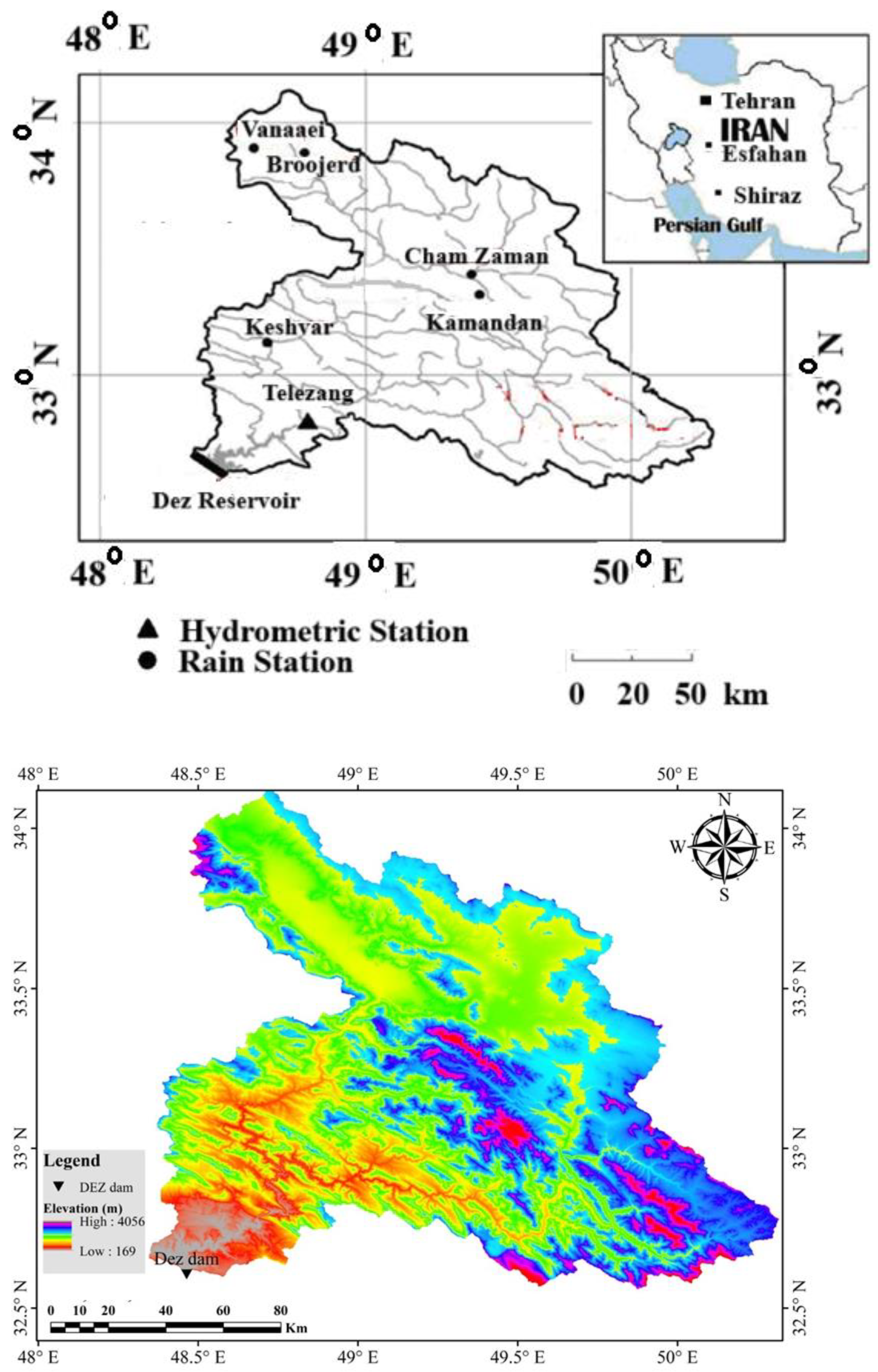
The Dez River watershed spans a geographical area between 48°10′ and 50°21′ East longitude and 31°34′ and 34°7′ North latitude. Encompassing a total area of 21,720 km², the watershed exhibits elevations ranging from 169 to 4056 m above sea level. The area of the Dez River watershed upstream of the Dez Dam is 17,365 km², which is approximately 1% of the total area of Iran. The general slope and direction of flow in the Dez River watershed is from north to south. The Dez watershed and locations of the synoptic and hydrometric stations are illustrated in Figure 1.

The mean monthly of flow discharge in the Telezang hydrometric station and mean monthly of precipitation and temperature (based on observed data in 22 synoptic stations) in the Dez watershed are shown in

Table 1. The mean monthly and annual of flow discharge, precipitation, and temperature in the Dez watershed.

Month	January	February	March	April	May	June	July	August	September	October	November	December	Annual.
Flow discharge (1955–2018) (m3/s)	219	298	463	559	398	215	138	94	73	70	118	186	236
Precipitation (1970–2018) (mm)	91.7	73.3	89.5	84.9	44.8	10.4	6.9	6.7	3.3	24.6	59.3	85.9	581.4
Temperature (1990–2018) (°C)	4	6	10.7	15.9	20.5	24.8	28.5	27.4	22.3	16.8	10.8	6.3	16.2

. The mean monthly precipitation and temperature were calculated with Thiessen’s method.

2.2. The Used Data

In this study, flow discharge data from the Telezang hydrometric station from 1955 to 2018 were used. For temperature and precipitation, data from synoptic stations shown in Figure 1 were utilized. After examining the temperature and precipitation data, an attempt was made to use stations with the most data and the fewest gaps. The precipitation data covers the period from 1970 to 2018, and the temperature data covers the period from 1990 to 2018. It is worth mentioning that, initially, these stations were rainfall gauging stations, and in the 1980s, after the end of the Iran–Iraq war, dam construction and development activities in this region increased significantly. The need for measuring other climatic variables, such as temperature, evaporation, and relative humidity for dam construction, agricultural, and water resource studies, became strongly felt. For this reason, these rainfall gauging stations were converted into synoptic stations. To address data gaps within the time series, the double mass method was applied. To achieve this, data from the station with the strongest correlation to the target station, which is usually the nearest station, were used. The used formula for the double mass method is:

$${CC}_i={CR}_i{\displaystyle \frac{\overline{{CC}_i}}{\overline{{CR}_i}}}$$

(1)

where C is climatic variable, C is considered station, R is reference station and i is month. It is important to note that the missing data constituted less than 1% of the overall dataset and had a negligible impact on the model’s outcomes. Due to the shorter time series of precipitation and temperature data compared to the flow discharge data, the APHRODITE dataset and CRU dataset were used to extend the statistical period of the precipitation and temperature time series, respectively. The APHRODITE dataset is suitable for Asia (Iran is located in Asia) and the precipitation outputs of this dataset have the best fitness with the observed precipitation. The time period of this dataset is 1901–2007 with spatial resolution 50 × 25 km (see http://www.chikyu.ac.jp/precip/english/products.html accessed on 25 August 2010). The time period of the CRU dataset is 1901–2017 with spatial resolution 50 × 25 km spatial resolution 50 × 50 km (see https://crudata.uea.ac.uk/cru/data/hrg/ accessed on 17 March 2021). The CRU dataset covers the entire globe. These datasets exhibited the highest correlation and the lowest root mean square error (RMSE) compared to the observed precipitation and temperature data at the stations within the Dez watershed. Other meteorological datasets, such as the ECMWF reanalysis 5th generation (ERA5), showed less agreement with the observed meteorological data at the stations within the Dez watershed [36]. 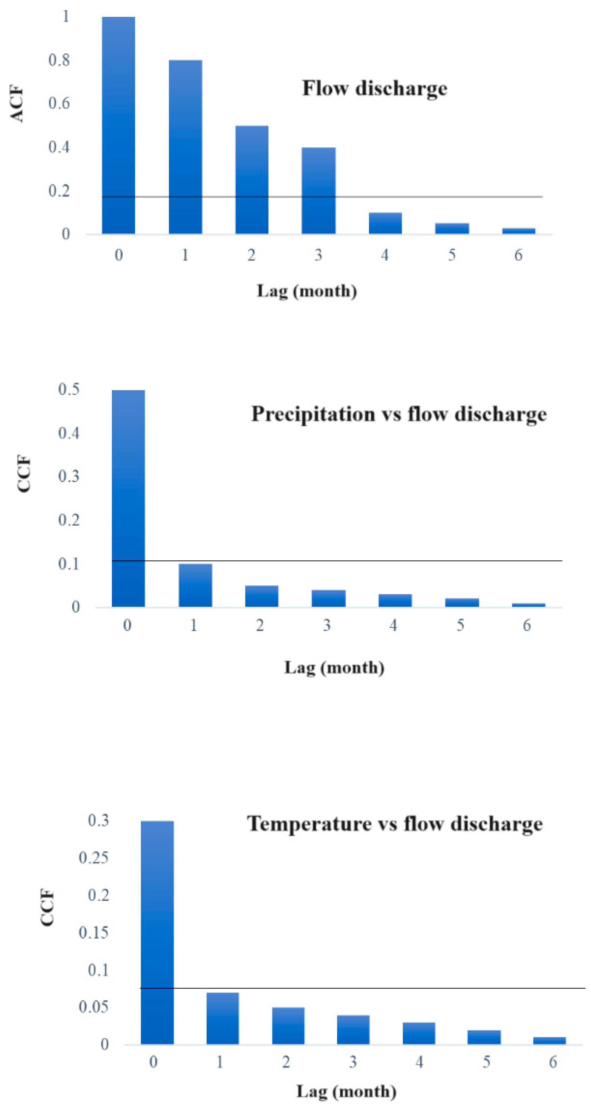The RMSE values and correlation coefficients for the APHRODITE precipitation dataset were R² > 0.90 and RMSE < 10 mm, and for the CRU temperature dataset, they were R² > 0.95 and RMSE < 0.3 °C. For selecting suitable input data for the models, the autocorrelation function (ACF) and cross-correlation function (CCF) have been used. ACF diagrams for flow discharge and CCF diagrams for temperature and precipitation against flow discharge were drawn. These diagrams show the time lag of each variable that can affect the flow discharge in the current month, t (Figure 2). This diagram shows that suitable data for models are P(t), T(t), Q(t-1), Q(t-2), and Q(t-3). Based on appropriate data, three combinations for inputs of models were considered.

• P(t), T(t), Q(t-1), Q(t-2), and Q(t-3)
• Q(t-1), Q(t-2), and Q(t-3)
• P(t) and T(t)

To reduce the effect of very large and very small data on the results in this research, the min-max normalization method was used to place the data in the range of zero to one.

2.3. Selection of Synoptic Stations and Extraction of Rainfall and Temperature Data in the Dez Watershed

In this study, 22 synoptic stations were considered, of which six stations had long-term data. These six stations are:

Telezang, situated at 48°46′ East, 32°49′ North with an elevation of 463 m. Broojerd, located at 48°46′ East, 33°53′ North and reaching an altitude of 1560 m. Vanaaei, positioned at 48°36′ East, 33°55′ North with an elevation of 1980 m. Cham Zaman, found at 49°24′ East, 33°24′ North and elevated to 1830 m. Kamandan, situated at 49°25′5″ East, 33°18′ North with an elevation of 1930 m. Keshvar, located at 48°42′18″ East, 33°8′57″ North and reaching an altitude of 770 m. Within the geographical boundaries of Telezang, Broojerd, Cham Zaman, Kamandan, and Keshvar stations, there are respectively five, two, two, four, and three sub-stations. The names (elevations) and geographic coordinates of these sub-stations are as follows:

Telezang: Dez Dam (525 m); Dezful (143 m); Safiabad Dezful (82.9 m); Tang Pang-Bakhtiari (540 m); and Shoul abad (165 m) from 32°16′ to 33°12′ North and from 48°23′ to 48°52′ East.

Broojerd: Rahimabad-Seilakhoor (1490 m) and Malayer (1777.8 m) from 33°47′ to 34°15′ North and from 48°48′ to 48°51′ East.

Cham Zaman: Ali Goudarz (2022 m) and Golpaigan (1870 m) from 33°24′ to 33°28′ North and from 49°42′ to 50°17′ East.

Kamandan: Dare Takht (1940 m); Kazemabad-Bakhtiari (2000 m); Zarde Fahre (2441 m); and Charkhfalak-Sibak (2552 m) from 32°53′ to 33°23′ North and from 49°23′ to 50°4′ East.

Keshvar: Cham Chit-Sabzeh (1290 m); Sepid Dasht-Sezar (970 m); and Khorramabad (1147.8 m) from 33°13′ to 33°34′ North and from 48° 17′ to 48°59′ East.

After completing the climatic time series data using the double mass method, these data were extended using data from the APHRODITE and CRU datasets. By determining the center of gravity of the geographical area of Telezang, Broojerd, Cham Zaman, Kamandan, and Keshvar stations using Arc GIS, the mean monthly temperature and precipitation in the Dez watershed were calculated as follows:

In each geographical area, the mean monthly precipitation and temperature at the centroid of the area are determined using the inverse distance weighting (IDW) method. Finally, these values are interpolated across the entire watershed using the Thiessen polygon method. The following points should be considered during this process:

• The variations in precipitation and temperature among the stations within each geographical area were not significant, and it was possible to use the data from the base station within the geographical area with acceptable accuracy.
• Since the variations in precipitation and temperature were slightly higher in lower-elevation areas compared to higher-elevation areas, an effort was made to place more sub-stations in these areas, specifically around the Telezang and Keshvar stations.

2.4. The Recurrent Neural Networks

LSTM:

LSTMs, introduced in 1997 for natural language processing, have gained significant recognition for their exceptional ability to remember long-term dependencies [37]. While sharing a similar chain-like structure with RNNs, LSTM cells possess a more intricate internal mechanism, enabling them to learn long-term dependencies. Unlike traditional RNNs, LSTMs introduce a specialized cell state capable of storing information. This cell state is meticulously regulated by three distinct gates: The forget gate selectively discards irrelevant information, while the input gate regulates the incorporation of new data; and the output gate, which specifies the information to be used as output. These gates function as selective filters, each with a specific role [38]. By employing this sophisticated architecture, LSTM cells excel at capturing intricate patterns in both short-term and long-term time series data, significantly surpassing the capabilities of traditional RNNs. (for details see [10]).

GRU:

Due to their intricate structure, training LSTMs can be computationally expensive and time-consuming. To address this, GRU was introduced as a simplified version of LSTM. GRU merges the hidden state and cell state, reducing the complexity of the network. GRU is controlled by two gates:

The update gate regulates the flow of new information into the hidden state; and the reset gate controls the amount of past information to be preserved [39].

Stacked LSTM:

The concept of deep neural networks involves stacking multiple layers of nonlinear transformations to learn hierarchical features. In a Stacked LSTM, the output of a hidden layer is not only propagated forward in time but also serves as an input to the subsequent LSTM layer [40].

Bi-LSTM:

Unlike unidirectional LSTMs, which process information sequentially, Bi-LSTMs consider data from both past and future time steps. This architecture employs two separate hidden layers: one processing the input sequence forward; and the other backward. By combining the outputs of these layers, Bi-LSTMs excel in tasks requiring comprehensive contextual understanding, often surpassing the performance of unidirectional LSTMs [1].

In this study, the used parameters in these models are: Epochs = 100; Batch size = 50; and N units = 100. These parameters were selected through a trial-and-error process. The selection criterion was the mean absolute error (MAE). To achieve this, the parameters were varied in increments of ten, and those that resulted in the lowest MAE were chosen. Since MAE was the selection criterion, the difference in MAE between the training and testing phases was negligible.

2.5. Pre-Processing of Data by Wavelet Transform

This study considered 21 Daubechies, 19 Symlets, five Coiflets, 15 Biorthogonal, 15 Reverse biorthogonal, and five Fejér–Korovkin and discrete Meyer (dmey) mother wavelet functions. After testing of these mother wavelet functions, it is observed that db5 is the best mother wavelet function (the obtained results by this mother wavelet function have the highest R² and lowest RMSE). The number of observed monthly data was 12 × 63 = 756. For training, 80% of data were used (604 data) while 20% of the data were used for tasting (152 data). It is worth mentioning that the trial-and-error method was used to determine the number of data points for the training and testing stages, by examining ratios of 60–40, 65–35, 70–30, 75–25, 80–20, and 85–15. Additionally, the selected data were continuously chosen from different sections of the time series. In this study, 756 data points were available. For instance, in the 80–20 ratio, 152 data points were considered for testing, and the data points selected for testing were numbered as follows: 1–152, 153–304, 305–456, 457–608, and 605–756. Ultimately, the ratio and dataset that showed the lowest average MAE in the training and testing stages were selected.

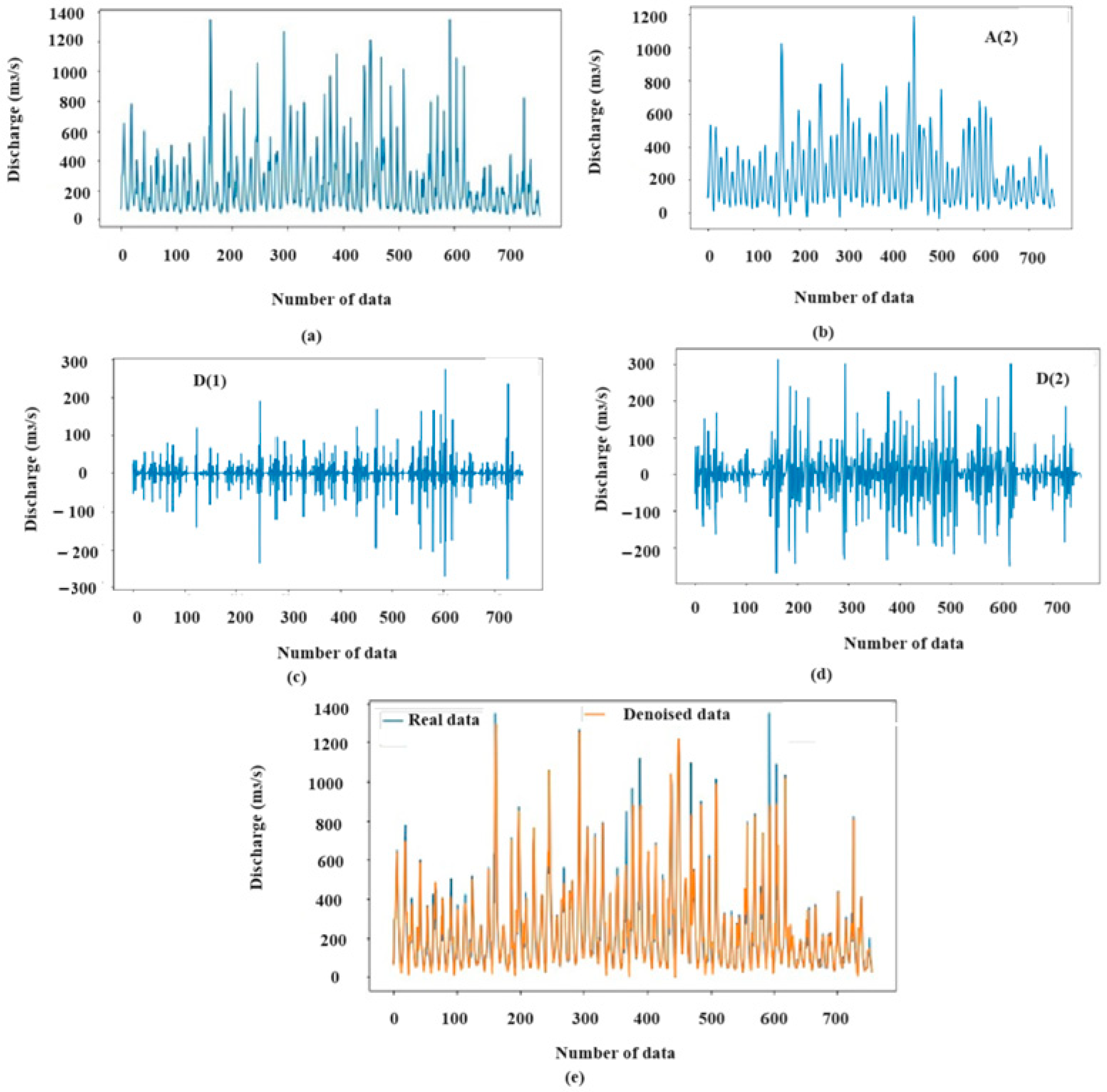
The relationship used to select the appropriate decomposition level using wavelets was L = Int (LogN), where L represents the decomposition level and N denotes the number of observed data. In this study N = 756 and L = 2. Figure 3 displays the application of the db5 mother wavelet to streamflow data at the second level of decomposition.

2.6. Uncertainty Analysis

This study used p-factor and r-factor for uncertainty analysis. The p-factor indicates the proportion of calculated values captured within the 95PPU, while the r-factor measures the width of this interval.

$$r-factor={\displaystyle \frac{\frac{1}{n}{\sum }_{i=1}^n{\left(C_u-C_l\right)}_i}{{\delta }_{obs}}}$$

(2)

n is the number of calculated values, Cu and C_l are the 97.5th and 2.5th percentiles of the model’s calculated values, respectively. ${\delta }_{obs}$ is the standard deviation of the calculated values (for details see [41,42]). Abbaspour [43] stated that p-factor > 70%, r-factor < 1.5 are acceptable values for prediction of flow discharge.

2.7. Performance Criteria

The used performance criteria in this study are:

Root mean square error (m³/s):

$$RMSE=\sqrt{{\displaystyle \frac{1}{n}}{\displaystyle \sum _{i=1}^n{(Q_{cal}^i-Q_{obs}^i)}^2}}$$

(3)

Mean absolute error (m³/s):

$$MAE={\displaystyle \frac{{\sum }_{i=1}^n\left|Q_{cal}^i-Q_{obs}^i\right|}{n}}$$

(4)

The Nash–Sutcliffe model efficiency coefficient:

$$NSE=1-{\displaystyle \frac{{\sum }_{i=1}^N(Q_{cal}^i-Q_{obs}^i{)}^2}{{\sum }_{i=1}^N(Q_{obs}^i-\overline{Q_{obs}}{)}^2}}$$

(5)

Coefficient of determination:

$$R^2={\displaystyle \frac{{\sum }_{i=1}^n(Q_{cal}^i-\overline{Q_{cal}}\left)\right(Q_{obs}^i-\overline{Q_{obs}})}{\sqrt{{\sum }_{i=1}^n(Q_{cal}^i-\overline{Q_{cal}}{)}^2(Q_{obs}^i-\overline{Q_{obs}}}{)}^2}}$$

(6)

Q_cal is calculated flow discharge (m³/s) and Q_obs is observed flow discharge (m³/s). $\overline{Q_{cal}}$ is the mean of calculated flow discharges (m³/s) and $\overline{Q_{obs}}$ is the mean of observed flow discharges (m³/s).

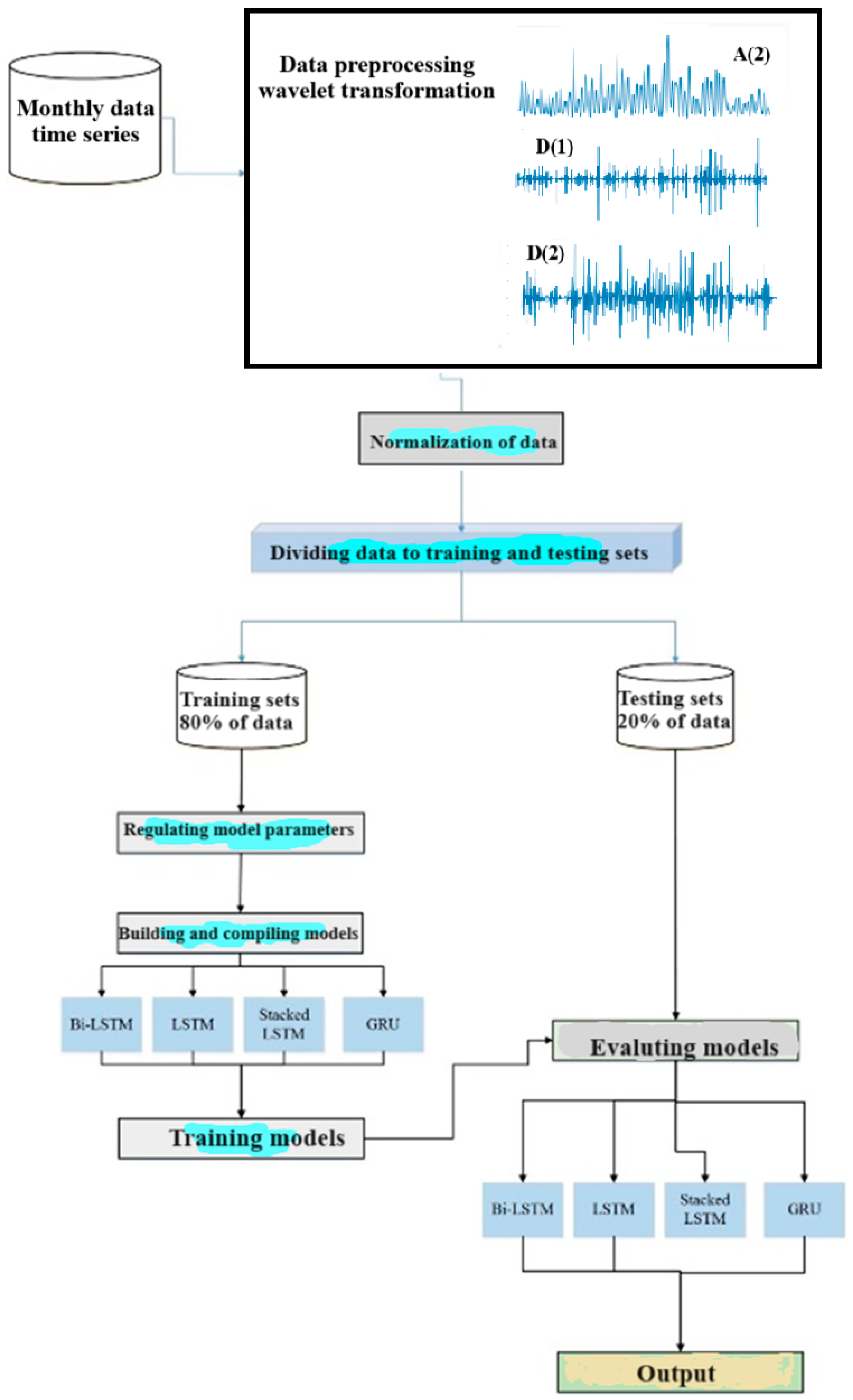
2.8. Research Methodology

The flow discharge data in the Tele Zang hydrometric station (63 years) and the temperature and precipitation data from synoptic stations upstream of the Dez Dam were used. By integrating data of hydrometric and synoptic stations and Asian precipitation and highly resolved observational data integration toward evaluation (APHRODITE) and climatic research unit (CRU), simulations were conducted using RNNs. To eliminate noise and increase prediction accuracy, WT was employed. Finally, the modeling uncertainty was calculated for the model that demonstrated the best performance. Figure 4 illustrates the research methodology employed in this study.

3. Results

The best RNN model is the GRU model for simulation of monthly flow discharge in this study (

Table 2. Performance criteria of different RNNs.

Model	Training				Testing
	RMSE (m3/s)	MAE (m3/s)	NSE	R2	RMSE (m3/s)	MAE (m3/s)	NSE	R2
LSTM	0.09	0.052	0.687	0.735	0.066	0.043	0.553	0.581
Stacked LSTM	0.089	0.052	0.644	0.741	0.07	0.048	0.522	0.44
GRU	0.083	0.047	0.746	0.774	0.061	0.038	0.556	0.642
Bi-LSTM	0.095	0.062	0.681	0.705	0.076	0.055	0.37	0.439

). The inputs of the models were P(t), T(t), Q(t-1), Q(t-2), and Q(t-3).

Table 2 shows that the GRU model is the best model for simulation of monthly flow discharge. The LSTM, Stacked LSTM, and Bi-LSTM models are in the next ranks, respectively. In the case of using Q(t-1), Q(t-2), and Q(t-3) as input data for the models, the values of RMSE, MAE, NSE, and R² are 0.086 m³/s, 0.052 m³/s, 0.721, and 0.756 in training stage and 0.07 m³/s, 0.046 m³/s, 0.481, 0.523 in testing stage for GRU (the best model). In the case of using P(t) and T(t) as input data for the models, the values of RMSE, MAE, NSE, and R² are 0.107 m³/s, 0.074 m³/s, 0.664, and 0.755 in training stage and 0.081 m³/s, 0.063 m³/s, 0.386, 0.437 in testing stage for GRU (the best model). Using meteorological data (precipitation and temperature) can improve performance of RNNs in testing stage while the effect of these data is negligible in training stage. These results show flow discharge data are the most important input to RNNs. Therefore, the lack of meteorological data does not significantly affect the results, and it is possible to predict the flow discharge with acceptable accuracy in watersheds without meteorological data.

For improvement of performance of different RNNs, this study utilized WT for pre-processing of data. After pre-processing of data by WT, it is observed that Bi-LSTM is the best RNN model (

Table 3. Performance criteria of different RNNs after pre-processing of data by WT.

Model	Training				Testing
	RMSE (m3/s)	MAE (m3/s)	NSE	R2	RMSE (m3/s)	MAE (m3/s)	NSE	R2
LSTM	0.013	0.009	0.997	0.998	0.019	0.013	0.996	0.995
Stacked LSTM	0.016	0.012	0.994	0.9986	0.024	0.015	0.992	0.989
GRU	0.022	0.017	0.986	0.9948	0.031	0.019	0.9647	0.9697
Bi-LSTM	0.011	0.007	0.9989	0.9989	0.014	0.008	0.9983	0.9981

). The inputs of the models were P(t), T(t), Q(t-1), Q(t-2), and Q(t-3) and the mother wavelet function was db5.

LSTM, Stacked LSTM, and GRU models are in the next ranks, respectively. In training stage, WT decreased RMSE and MAE 87% and 85%, respectively, and increased NSE and R² 34% and 29%, respectively. In testing stage, WT decreased RMSE and MAE 77% and 79%, respectively, and increased NSE and R² 80% and 55%, respectively. As previously mentioned, the best wavelet mother function in this study was db5.

Table 4. Performance criteria of a number of used mother wavelet functions for pre-processing of data.

Mother Wavelet Function	Training				Testing
	RMSE (m3/s)	MAE (m3/s)	NSE	R2	RMSE (m3/s)	MAE (m3/s)	NSE	R2
db2	0.013	0.011	0.994	0.993	0.016	0.014	0.985	0.983
Haar	0.041	0.018	0.89	0.902	0.06	0.024	0.837	0.851
sym2	0.013	0.009	0.997	0.9981	0.021	0.015	0.984	0.983
sym5	0.013	0.008	0.9978	0.9978	0.017	0.013	0.991	0.986

shows the best results obtained from several wavelet mother functions.

After db5, sym5 is the best mother wavelet function. Therefore, the best model for predicting monthly flow discharge without using wavelet is the GRU model, and when using wavelet, it is the Bi-LSTM model. In the case of using Q(t-1), Q(t-2), and Q(t-3) as input data for the models, the values of RMSE, MAE, NSE, and R² are 0.031 m³/s, 0.024 m³/s, 0.892, and 0.894 in training stage and 0.034 m³/s, 0.03 m³/s, 0.8533, and 0.8309 in testing stage for Bi-LSTM with db5 wavelet mother function (the best model). In training stage, WT decreased RMSE and MAE 64% and 54%, respectively, and increased NSE and R² 24% and 18%, respectively. In testing stage, WT decreased RMSE and MAE 51% and 35%, respectively, and increased NSE and R² 77% and 59%, respectively.

In the case of using P(t) and T(t) as input data for the models, the values of RMSE, MAE, NSE, and R² are 0.059 m³/s, 0.038 m³/s, 0.772, and 0.7918 in training stage and 0.063 m³/s, 0.041 m³/s, 0.5094, and 0.5395 in testing stage for Bi-LSTM with db5 wavelet mother function (the best model). In training stage, WT decreased RMSE and MAE 45% and 49%, respectively, and increased NSE and R² 16% and 5%, respectively. In testing stage, WT decreased RMSE and MAE 22% and 35%, respectively, and increased NSE and R² 32% and 23%, respectively.

In the case of using P(t), T(t), Q(t-1), Q(t-2), and Q(t-3), The accuracy of RNNs is low in the absence of wavelet pre-processing (NSE is between 0.37 to 0.556 in testing stage). However, the accuracy of the models increases significantly with wavelet pre-processing (NSE is between 0.9647 to 0.9983 in testing stage). The wavelet pre-processing’s high-pass filter incorporates information from future time steps, influenced by the mother wavelet’s properties. For example, when using the db4 mother wavelet function, the pre-processing technique incorporates data from previous time points. At decomposition level 1, this includes information from the past 2.8 days. 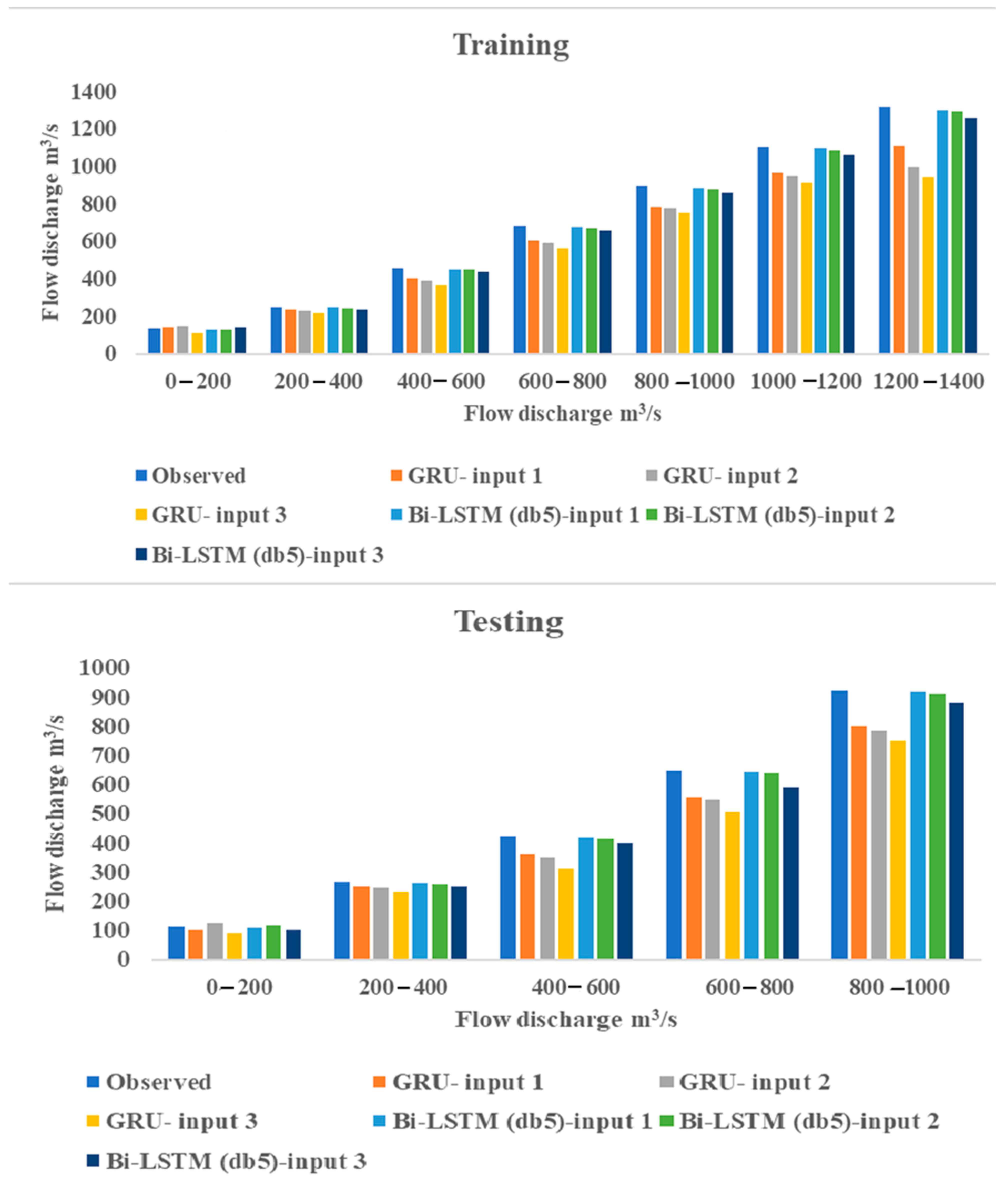At level 2, it extends to 5.6 days, and at level 8, it captures data from the preceding 358 days [44,45]. The accuracy of RNNs does not improve as much with wavelet preprocessing when only P(t) and T(t) are used, since these variables do not incorporate past data. Therefore, to solve this problem and achieve acceptable accuracy, using Q(t-1), Q(t-2), and Q(t-3) can be used to predict Q(t). Additionally, in this study, level 2 decomposition has been used, and the goal is to predict the monthly flow discharge. Pre-processing using wavelets at this level is not capable of retaining monthly information. Furthermore, in the Dez River, due to the fact that both rainfall and snowmelt are factors contributing to floods, and sometimes severe floods occur (such as the flood in May 2016), in high discharges that occur suddenly, there is not much correlation between consecutive monthly time steps. The main advantage of pre-processing with wavelets, which is the accurate simulation of high discharges, demonstrates its importance (Figure 5). Figure 5 presents a comparison of observed and modeled values during both training and testing phases.

For the creation of Figure 5, the monthly discharge flow data collected at the Telezang station (comprising 756 data points) were categorized into seven distinct classes. Each class has a range of 200 cubic meters per second. The distribution of data points across these classes is as follows: 539, 116, 49, 17, 16, 12, and seven data points, respectively.

Figure 5 is constructed by calculating the average value for each class. The values produced by the various models were also averaged and incorporated into this plot. This approach allows for a direct comparison between the observed data and the data generated by each model. Consequently, the optimal model and the most suitable set of input data for the model can be determined. In this figure, the set of input data 1 includes P(t), T(t), Q(t-1), Q(t-2), and Q(t-3); the set of input data 2 includes Q(t-1), Q(t-2), and Q(t-3) and the set of input data 3 includes P(t) and T(t).

Figure 5 demonstrates that the agreement between the observed data and the computed values is significantly improved when WT is used for pre-processing the data. The main advantage of using WT is the simulation of maximum flow discharge values. To analyze uncertainty, a GRU model was chosen for scenarios without wavelet-based data pre-processing. In contrast, a Bi-LSTM model employing the db5 mother wavelet function was selected for cases involving wavelet-preprocessed data.

Uncertainty analysis:

Model output uncertainty was assessed using the 95% prediction uncertainty (95PPU) band, p-factor, and r-factor. For each observed data point, a 95% confidence interval was calculated. The width of this interval represents the model’s uncertainty in predicting that specific value. The p-factor indicates the proportion of observed values that fall within their respective confidence intervals. The r-factor is computed by dividing the average width of these intervals by the standard deviation of the observed data.

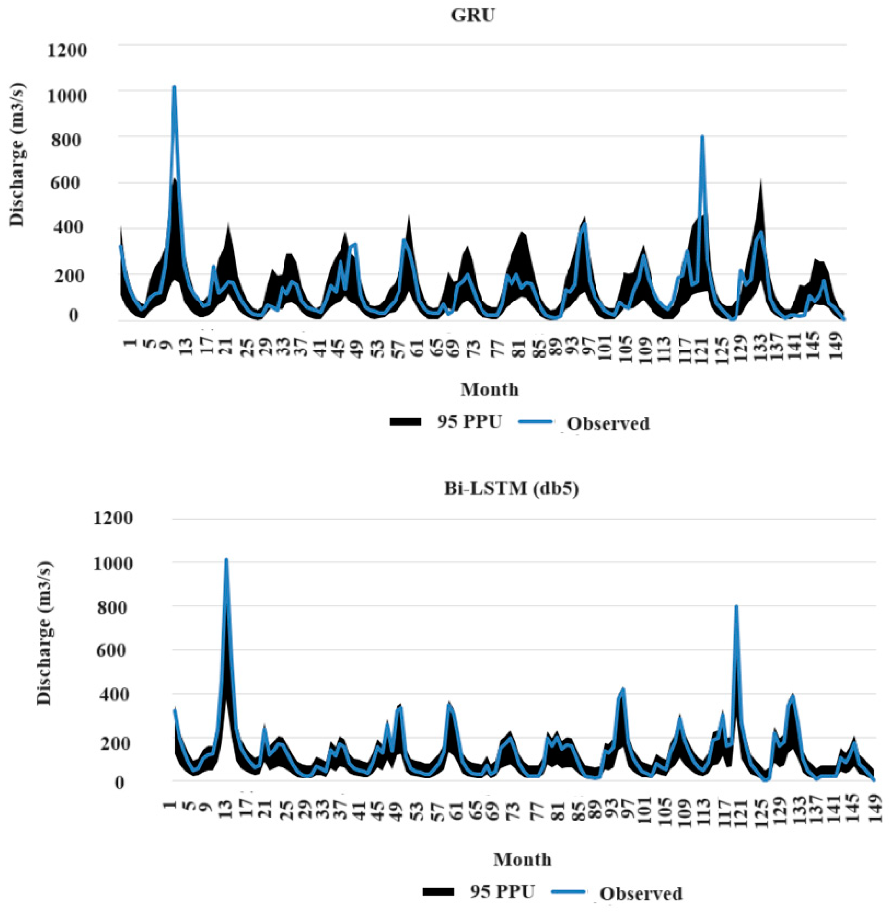
The GRU and Bi-LSTM models achieved p-factor values of 82% and 94%, respectively. These results are considered satisfactory, as they demonstrate that a large proportion of observed data points lie within the 95% prediction interval. For reliable p-factors, r-factors must be below a certain threshold. The GRU and Bi-LSTM models, with r-factors of 1.28 and 1.06, respectively, meet the criteria for flow discharge data (p-factor > 70%, r-factor < 1.5). The 95PPU range of the calculated flow discharges for the two mentioned models in the testing stage is shown in Figure 6. Pre-processing data by WT increases p-factor 15% and decreases r-factor 16%.

Figure 6 shows that pre-processing the data using WT decreases the uncertainty associated with the computed values. Consequently, a larger percentage of the observed data fall within the 95PPU. This is particularly evident for maximum flow discharge values.

The Dez River has multiple tributaries, including the Sazar, Bakhtiari, and Tireh, situated in mountainous areas with steep gradients. These geographic conditions often result in significant water flow during flood events. Consequently, the Dez River experiences large flow discharges more frequently than its average flow. To enhance the accuracy of predicting these large flow discharges, pre-processing the data using a WT is crucial. This technique helps to reduce uncertainty in the forecasting process. In 1968 and 1979 (corresponding to approximately months 150 and 280), the river witnessed severe floods. As illustrated in Figure 5, a combined model of RNN and WT effectively simulated these flood events. Due to the fact that very large flow discharge data in the Dez watershed are extremely rare (only seven data points exceeding 1200 m³/s, i.e., less than 1%) and these events occur suddenly (due to the mountainous nature and the presence of steep tributaries in the Dez watershed), RNNs do not receive sufficient training to simulate these data. 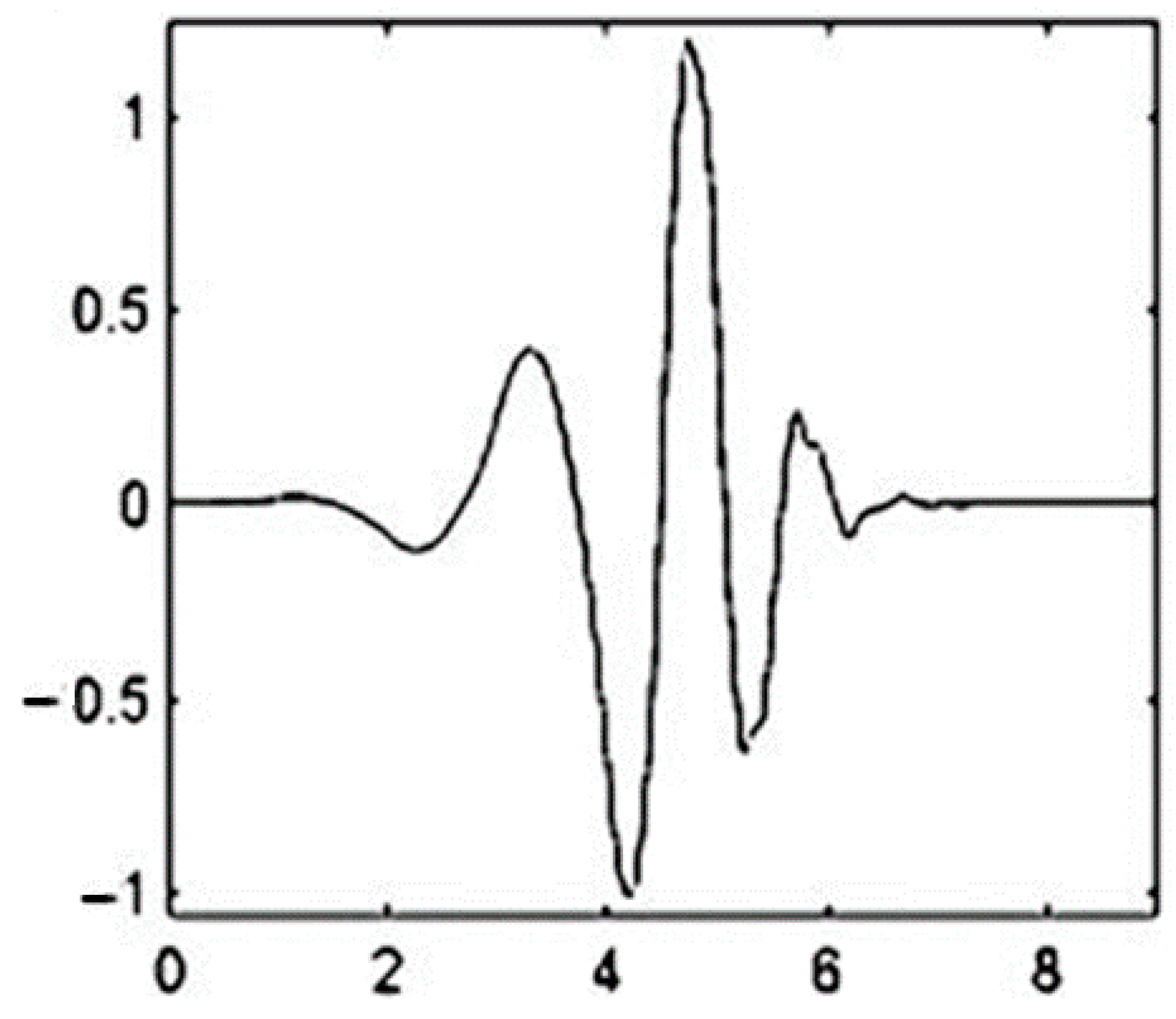On the other hand, for 704 data points (over 93% of the data) with flow discharge less than 600 m³/s, these events do not occur suddenly, and therefore, the model receives sufficient training to simulate them. Thus, the performance of RNNs is good for smaller data but weak for larger data. However, with pre-processing of the data with WT, since the db5 mother wavelet function is used, the shape of this function is such that it can simulate sudden changes in the data, and the occurrence of very large or small values suddenly aligns with its shape. The shape of this mother wavelet function is shown in Figure 7. For this reason, simulating large flow discharges that occur suddenly using a combination of RNNs with WT leads to satisfactory results [46].

4. Conclusions

The objective of this study was the determination of an integrated method (RNN and WT) for prediction of monthly flow discharge. By comparing four different types of RNNs, it was found that the GRU model has the highest performance for predicting flow discharge. The GRU has a simpler structure compared to other RNNs, which leads to the highest performance by this model in this study. This is due to the limited amount of input data to the RNN (five data). The use of GRU particularly increases the NSE and R² values. In the next step, by using data pre-processing through WT, the efficiency of RNNs increases. In this stage, the Bi-LSTM model has the highest efficiency. The reason for this is the nature of training this type of RNN, which is bidirectional (forward and backward), and the nature of this study, which is forecasting flow discharge from past hydrological and meteorological data. Noise reduction and smoothing of the time series data by WT also contribute to the superiority of this model. Using WT for pre-processing data particularly reduces the RMSE and MAE (almost 82%).

In this study, using the db5 mother wavelet function showed the best results, which is due to the compatibility of the shape of this mother wavelet function with the time series of flow discharge (Figure 5). These results are confirmed by Farajpanah [46] using a waveform matching algorithm. Using data pre-processing with WT reduces the uncertainty in flow discharge prediction by 15%. The r-factor and p-factor values indicate that the flow discharge predictions can be trusted when using the best models in this research. One of the positive aspects of using data pre-processing with WT is the increased accuracy of predicting flow discharges greater than 600 m³/s. If WT is not used, the predicted values of flow discharges greater than 600 m³/s are significantly lower than the actual values. Gao et al. [10] and Zhang et al. [47] demonstrated that, due to its simpler structure compared to LSTM, GRU is a better choice for flow discharge prediction, which corroborates the findings of this research.

The impact of climate change in the future on Middle Eastern countries will be greater than in other parts of the world, due to the presence of oil resources, land degradation, and a significant reduction in available water resources. Therefore, to predict streamflow in these regions, data should first be preprocessed using WT, and then streamflow should be predicted using AI methods. AI models alone are not capable of simulating extreme values, such as high flows resulting from severe floods or low flows resulting from severe droughts. The method used in the study is quite good, and gives relatively accurate results for the study area, therefore the results of this study are widely applicable in other watersheds located in arid and semi-arid regions.