Article

Predicting Flood Inundation after a Dike Breach Using a Long Short-Term Memory (LSTM) Neural Network

by
Leon S. Besseling
*,
Anouk Bomers
and
Suzanne J. M. H. Hulscher
Water Engineering and Management Department, University of Twente, 7500 AE Enschede, The Netherlands
*
Author to whom correspondence should be addressed.
Hydrology 2024, 11(9), 152; https://doi.org/10.3390/hydrology11090152
Submission received: 8 August 2024 / Revised: 2 September 2024 / Accepted: 4 September 2024 / Published: 12 September 2024

Abstract

:
Hydrodynamic models are often used to obtain insights into potential dike breaches, because dike breaches can have severe consequences. However, their high computational cost makes them unsuitable for real-time flood forecasting. Machine learning models are a promising alternative, as they offer reasonable accuracy at a significant reduction in computation time. In this study, we explore the effectiveness of a Long Short-Term Memory (LSTM) neural network in fast flood modelling for a dike breach in the Netherlands, using training data from a 1D–2D hydrodynamic model. The LSTM uses the outflow hydrograph of the dike breach as input and produces water depths on all grid cells in the hinterland for all time steps as output. The results show that the LSTM accurately reflects the behaviour of overland flow: from fast rising and high water depths near the breach to slowly rising and lower water depths further away. The water depth prediction is very accurate (MAE = 0.045 m, RMSE = 0.13 m), and the inundation extent closely matches that of the hydrodynamic model throughout the flood event (Critical Success Index = 94%). We conclude that machine learning techniques are suitable for fast modelling of the complex dynamics of dike breach floods.

1. Introduction

Floods are a problem that is experienced all over the world, and they are among the most destructive of all natural disasters [1,2]. Dike breaches along rivers are a type of flood that can have particularly sudden and severe consequences. This is a result of the unexpected nature of the event, the rapid breach outflow [3], as well as high densities of people and economic assets in hinterlands [4]. Breaches occur when hydraulic loads exerted by a river discharge wave exceed the resistance capacity of the dike to failure mechanisms such as overtopping or piping. Water then erodes away the dike material and inundates the land behind the dike. Because of the unexpected nature and possibly severe consequences of these events, it is vital for public safety that these events are predicted and their flood consequences mapped.
Flood models are important tools that offer relevant information, such as flood depths, flood extents and flood arrival times [5]. They enable authorities to make informed decisions on measures such as timely ordering of evacuation. In the case of an incoming extreme river discharge wave, these decisions have to be made under time pressure and with sufficient certainty about the risks [6,7]. Ensemble model predictions and uncertainty analysis of many model runs would allow for reviewing scenarios and making more informed decisions [5,6]. As such, a real-time flood forecasting system is desired that allows for fast modelling during a crisis situation.
Numerical simulation tools such as hydrodynamic models are often used for modelling dike breach floods. They generally utilize a one-dimensional (1D) part for flow in the river channel and a two-dimensional (2D) part for overland flow in the floodplain or hinterland (e.g., [4,8,9]). Such 1D–2D coupled hydrodynamic models represent the flow in the river and floodplain accurately, but they are computationally expensive due to their complex descriptions of the physical system [5,10]. Depending on the size of the study area, simulation times are often multiple hours, which makes the use of hydrodynamic models in a real-time flood forecasting system unfeasible [10,11].
A currently operational solution is to utilize a database of various flood scenarios [11,12], and such approaches are used in, for example, the Netherlands [13]. In case of an emergency, authorities select a flood event from the database that most resembles the current situation to assess the risks and advise policy makers, which can lead to relevant insights [14]. However, this method is limited to the scope or applicability of the scenarios created. As such, there is a need for faster modelling methods that can simulate flood scenarios in real time during an emergency situation.
Two general strategies towards faster flood modelling are distinguished. First, hydrodynamic models have recently seen computation time reductions as a result of developments regarding GPU-acceleration. For example, Vacondio et al. [15] achieve a speed-up of two orders of magnitude compared to a single-core CPU with their numerical scheme suitable for GPU. Morales-Hernández et al. [16] published an open-source GPU-based hydrodynamic model that in its lowest hardware configuration outperformed the most powerful CPU-based configuration that was tested. Both these studies conduct tests with millions of grid cells on high-resolution elevation maps (2×2 and 10×10 m, respectively) so larger speed-up factors could be possible with smaller domains and a lower grid resolution. Such schemes thus promise the application of hydrodynamic models to large-scale flood events in situations where simulation time is an important factor.
The second common approach for faster flood modelling is using one of two types of surrogate models [17]. First, lower-fidelity surrogates usually coarsen the model domain or leave out some physical characteristics of the system. Some purely conceptual models require only the digital elevation model of an area (e.g., [18]). Second, response surface surrogates are data-driven and do not contain representations of physical descriptions from the original complex models. Artificial Neural Networks (ANNs) are the most commonly used response surface surrogate model [2]. They are trained to find relations between the input and output of another model or field data, in order to make their own predictions for a new set of input. An advantage of neural networks especially relevant to real-time flood forecasting is that their computation times are in the order of seconds to minutes. The focus of this paper will be on the ANN branch of the response surface surrogates, to make fast predictions of inundation water depths after dike breaches.
The first application of neural networks for flood modelling was the prediction of 1D flow in river channels, such as rainfall–runoff models (e.g., [19,20]). Over the past years, they have been increasingly applied to the prediction of 2D flood depths and flood extents as well [5,21,22]. This requires both a spatial and a temporal component to the prediction, and some of the most common deep learning models used are Recurrent Neural Networks (RNNs) [23]. Due to circular and self-feedback connections in this type of network, RNNs are more dynamic and more effective in time series problems [24].
Most studies using neural networks model floods caused by rivers spilling gradually into the floodplains (e.g., [5,25,26]). Inundation due to dike breaches remains a largely unexplored field of study [23], and these events contain challenging aspects to model. First, river discharge waves that cause breaches can differ in both peak discharge and flood wave duration. This affects the flood volumes that flow through the breach and thus the subsequent flood propagation in the hinterland. Second, there is a large spatio-temporal variation in the water depth patterns that emerge after a dike breach. Close to the breach, the sudden high discharge of water entering the hinterland leads to water depths rising exceptionally fast. However, further away from the breach, the flow velocities are lower and the water depths increase less rapidly.
The objective of this paper is to create an accurate neural network for predicting maps of water depths in time for a large-scale flood after a dike breach. The IJssel distributary of the Rhine river in the Netherlands is used as a case study area, to ensure that the neural network is operational for realistic circumstances. No detailed data of historic flood events exist for this area, so overland flow data from a calibrated and validated 1D–2D hydrodynamic model by Bomers [27] are used for the training data. The research focuses on the capability of neural networks to learn and predict the flood water depths in the hinterland, especially the spatial and temporal depth variations that occur near and far from the breach. The main research question is as follows: what is the accuracy as well as the practicality of a neural network for use in a real-time flood forecasting system for dike breaches?
This paper is structured as follows. First, an explanation of neural networks and the choice for the specific network type is provided (Section 2). Then, the case study area and the hydrodynamic model used for generating training data are introduced (Section 3). The neural network is set up and the methods for training and evaluation are defined (Section 4). The results cover the testing of the neural network on a set of unseen flood scenarios not used in the training procedure (Section 5). Finally, the paper discusses the model, its application and future research directions (Section 6), and it ends with the conclusion (Section 7).

2. Neural Networks

In this study, a neural network called a Long-Short Term Memory (LSTM) is used for flood prediction. This neural network is known to be successful in the prediction of time series [28]. Here, we shortly summarize the principles of neural networks, to explain how an LSTM functions.

2.1. Neural Networks in General

Neural networks are data-driven models that generate an output based on a set of input parameters. They consist of interconnected neurons, organized in sets of layers. Each neuron receives information through the input data or through neurons in previous layers. Therefore, these simple networks are called feed-forward neural networks. Each neuron assigns a weight to each of its inputs and calculates its output to the next neurons through an activation function specified by the modeller. Common activation functions are, for example, the linear function, rectilinear function, sigmoid function and hyperbolic tangent function.
The training of the neural network is conducted by repeatedly presenting the network with an input and a corresponding desired output. The network initializes with randomized weight factors and computes its own output from the input [24]. The error between the desired and observed output is calculated using a loss function specified by the modeller, such as the Mean Absolute Error (MAE), Root Mean Square Error (RMSE) or a custom loss function. Then, the weights of each input for each neuron are slightly changed. There are several methods for this, but usually backpropagation is used in combination with a stochastic gradient descent algorithm [28]. The updated neural network is again presented with input and corresponding output values, and the cycle repeats. Each of these training cycles is called an epoch and leads to a slightly better prediction. The training process stops when convergence is achieved, i.e., when the loss function does not improve over a set amount of epochs.

2.2. Recurrent Neural Networks

Feed-forward neural networks have independent input and output, meaning that the results of one computation are not automatically used for the next computation. Recurrent Neural Networks (RNNs) were developed to have an additional set of neurons with circular and self-feedback connections, allowing information to be stored and used for the next computation step [29]. This gives the network a kind of memory and allows it to be much more effective in sequential data problems such as time series prediction [24].
However, simple RNNs are not sufficiently efficient to recognize and learn long-term dependencies in data [28]. This is because after a period of training, the backpropagation of errors leads to the error gradient either growing or shrinking with every time step. Referred to as the exploding or vanishing gradient problem, it causes the training process to become unstably oscillating or very time-consuming, respectively. As a consequence, a standard RNN cannot effectively learn dependencies of information of more than 5–10 time steps [24].

2.3. Long Short-Term Memory

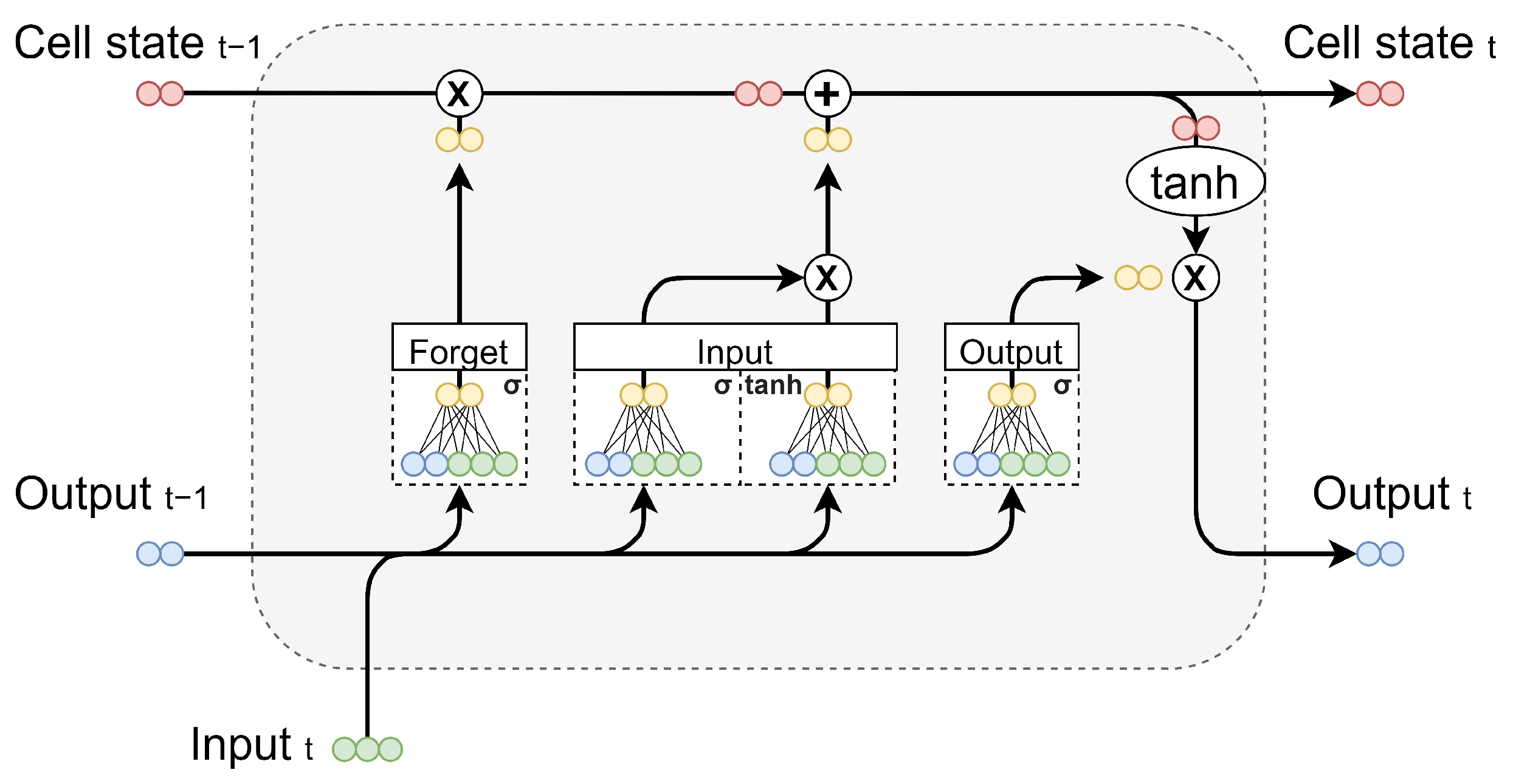
The Long Short-Term Memory (LSTM, Figure 1) neural network proposed by Hochreiter and Schmidhuber [30] is a type of RNN that solves the vanishing gradient problem. We provide here a short description of the structure of the LSTM. For readers interested in the mathematical model besides that in the introduction paper by Hochreiter and Schmidhuber, we would like to refer to three excellent articles discussing the development and evolution of the LSTM neural network: Sherstinsky [31], Staudemeyer and Morris [24] and Yu et al. [29].
The LSTM neural network considers three streams of data to compute the result for each time step: (1) the input features that are given by the modeller, (2) the output that the LSTM has computed from a previous time step, named the hidden state, (3) the dedicated memory for the network, referred to as the cell state [29]. The three data streams pass through four gates and are combined in various addition or multiplication operations (Figure 1). Each gate is a neural node with trainable weights and specified activation functions [29]. They ensure a constant preservation of error and prevent vanishing gradients [24]. This way, information storage is achieved for much longer time periods than those of normal RNNs [30]. Due to the LSTM’s ability to learn such long-term dependencies, it has proven to be suitable for time series prediction (e.g., [28,32,33]).
Figure 1. The structure of an LSTM neural network, showing three data streams and four internal neural nodes functioning as the forget, input and output gates, here displayed with an input dimension of 3 and output dimension of 2. Reproduced from Karim [34].
Hydrology 11 00152 g001

3. Case Study

The study area of this research consists of the Rhine river delta in the Netherlands (Figure 2). The Rhine is one of the major rivers in Europe, originating in the Swiss Alps. The river flows through Germany to become a river delta in the Netherlands. Upon entering the Netherlands at Lobith, the river bifurcates into the Waal river and Pannerdensch Canal. This canal subsequently bifurcates into the Nederrijn and IJssel rivers.

3.1. Hydrodynamic Model

A coupled one-dimensional–two-dimensional (1D–2D) hydrodynamic model of the study area was created by Bomers et al. [8] in the software package HEC-RAS (version 5.0.3). The model was calibrated and validated using water level measurements of the 1995 and 1993 near-flood events in the Rhine. The model is used by Bomers [27] to predict outflow hydrographs of dike breaches in the bifurcating river system using neural networks. 1D–2D hydrodynamic model data from the study by Bomers [27] are available for this research on predicting overland flow using an LSTM neural network.

3.1.1. River and Hinterland

The upstream boundary of the hydrodynamic model is located at Emmerich in Germany (Figure 2). A discharge wave of interest can be used as the upstream boundary condition. The downstream boundary conditions are defined as the normal water depths in the rivers. This boundary condition computes the water depth through the Manning equation, using the specified cross-section, friction, energy slope (or approximation by bed slope) and the flow exiting the boundary. The river sections present in this area are discretized by 1D profiles, while the hinterland is represented as a 2D grid with a resolution of 150×150 m. To more accurately capture overland flow behaviour, the grid contains flexible cells to align itself with raised structures such as dikes and (rail)roads (Figure 2). Additionally, realistic Manning roughness values for the hinterland (e.g., 0.03 s/m1/3 for grasslands, 0.036 s/m1/3 for urban areas and 0.15 s/m1/3 for forests) are implemented based on land use information provided to Bomers [27] by the local authorities.

3.1.2. Dikes and Breaches

The connection between the 1D profile and 2D grid uses HEC-RAS lateral structures that represent the river dikes. Bomers [27] only includes overtopping as a failure mechanism, since it is the most common failure mechanism of modern dikes [7], and it requires less detailed information on dike characteristics. The breach growth is modelled as immediate: as soon as the water level is higher than the dike crest level, the crest level is reduced to the level of the natural terrain and a constant breach width of 150 m is assumed.

3.2. Available Data

Bomers [27] used discharge wave scenarios within a 95% confidence interval for the maximum design discharge of the Dutch Rhine river branches based on current climate conditions. This discharge corresponds to a return period of 100,000 years and results in peaks between 16,500 and 19,300 m3/s at the German–Dutch border. By varying the shape of the discharge waves to be longer or shorter, a varied selection of events was included in the data. From these data, 73 scenarios are available for this study.
Bomers [27] found that one location in the IJssel river breached during all discharge waves. This location (red cross in Figure 2) will be the focus of this research, to maximize the amount of available data. Note that Bomers [27] only published results of the outflow hydrograph data, so the overland flow data available for this research have not been published before. As part of this study, the data are made publicly available in a database (see Data Availability Statement).
The IJssel breach location is characterized by a flat topography, with a gentle downwards slope away from the breach. The flood water spreads from the breach in the south-west of the study area towards the north-east, covering the distance of approximately 35 km in 2 days. The surface elevation at the breach location is +11 m above mean sea level; the most downstream boundary of the hinterland in the model is at +7.5 m. The crest of the dike at the breach location is four meters above surface level. Land use in the area is mostly agricultural, but a town is located directly at the breach location.
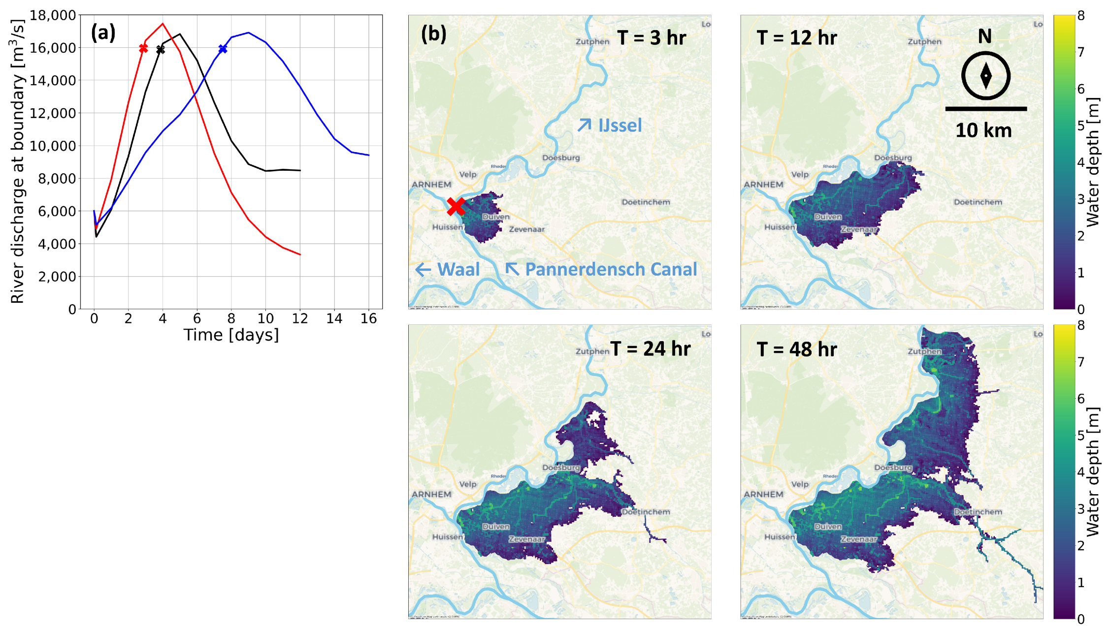
The overland flow data are available with a 3 h interval. Figure 3 shows four snapshots from a flood scenario for the IJssel breach location. Within the first time step of 3 h, the depths close to the breach rise to their maximum of 2 to 6 m depending on the local bathymetry. Further from the breach, the maximum depth of 2 to 4 m is reached about two days after water arrives in a particular location. These large differences in flood water behaviour near to and far from the breach will form an interesting case for researching the capabilities of the LSTM neural network.

3.3. Data Variability

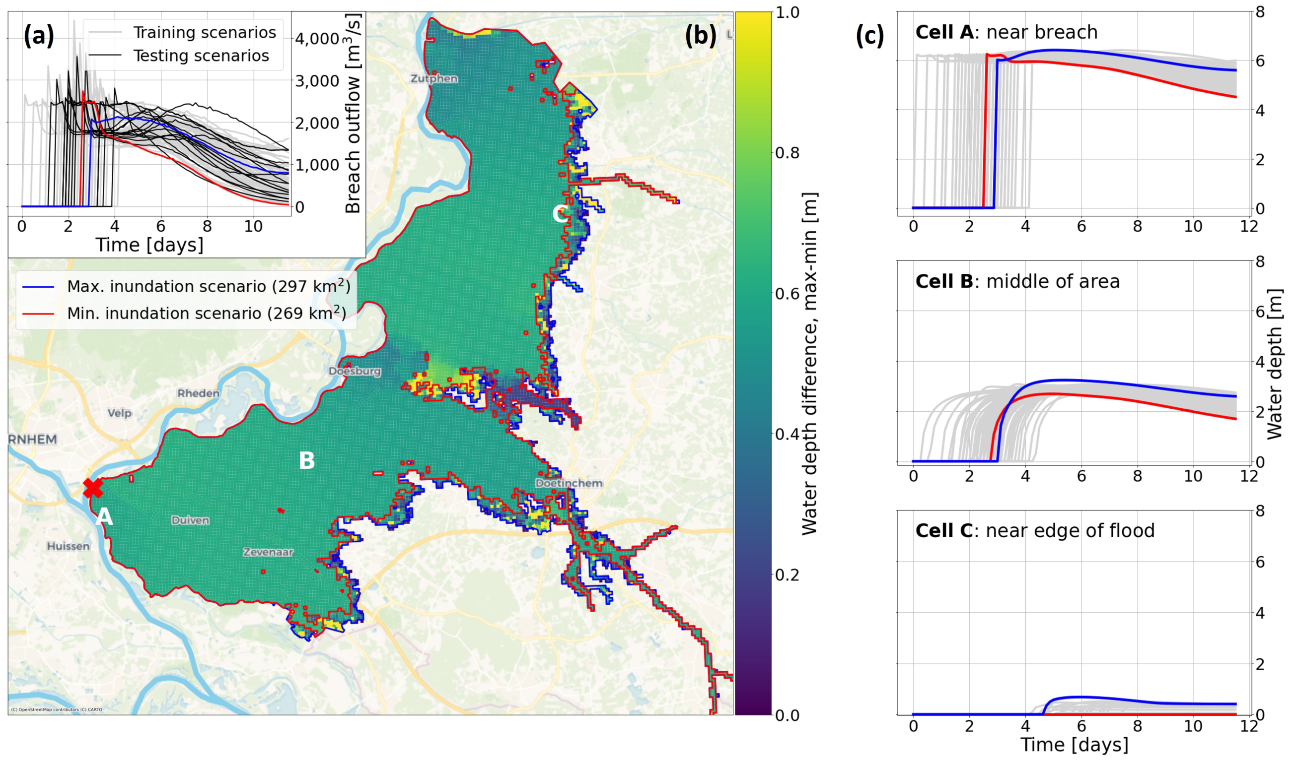
The available data of the 73 scenarios for the neural network training need to cover a sufficient range of possible flood events. The input data of the neural network consist of the breach discharges (Figure 4). The data are split into training and testing data, which is explained in more detail in Section 4.1.3. The output data of water depths result in the smallest final inundation extent of 269 km2 and the largest of 297 km2. The difference is found in an approximately 1 km further flooding inland around the flood edges (Figure 4). While the inundation extent of the flood is similar in these scenarios, some show quickly receding water depths because of a shorter flood wave, and others contain a longer increase in water depths due to a longer flood wave. The neural network’s capability to model this is discussed in Section 5.2.

4. Methods

4.1. LSTM Model Setup

One LSTM neural network was set up that predicts the water depths on all 34,629 grid cells throughout the duration of the simulation. The input it requires for this is a time series of the breach outflow hydrograph. As can be seen in Figure 4, the breaching moment is not equal for all the scenarios, which is due to the different discharge waves used as forcing in the hydrodynamic model. We could not shift the outflow hydrograph scenarios forwards all to start at the same time, since they require the same amount of time steps to enable LSTM training. Therefore, while the input of the neural network remains 0 and the flood has not yet started, we replace the neural network’s output with an all-zero output. This is because we are interested in how the network predicts flood propagation, not in how it converts 0 as input to 0 as output. We include a discussion on this in Section 6.1.
The neural network was created using the Keras library in Python [35], which acts as an interface for the TensorFlow open source machine learning and AI library developed by Google (version 2.6.0, [36]). The hardware used for this study is a laptop with an Intel Core i7-8750H CPU and an NVIDIA GTX-1060 GPU with 6 GB of VRAM.
The procedure of creating a neural network starts with choosing an appropriate network type and architecture. Next, the parameters and functions for the network training have to be chosen and optimized. Finally, the available data should be split into training, validation and testing data sets. Each of these steps is described below.

4.1.1. Choice of Architecture

The most simple form of LSTM consists of a single LSTM layer. The input is fed to the LSTM layer, and its output is connected to a standard Dense output layer. This output layer contains one neuron for each grid cell, enabling the model to make water depth predictions for the complete area. Tests were also conducted by inserting multiple LSTM layers before the Dense output layer. Such a setup possibly offers additional abstractions of the input over time and a deeper understanding of the relationship between input and output [29,37]. However, through initial testing, no significant difference was found between the performance of a single LSTM layer compared to two, three or four layers of LSTM. Thus, a single LSTM layer was chosen to maintain model simplicity.

4.1.2. Parameter Optimization

Four hyperparameters of the LSTM layer were optimized using the Bayesian optimization function of Keras. The first was the number of units, which is the dimensionality (number of neurons) of the hidden state and the cell state of the LSTM layer. The optimization was run between a minimum of 16 and a maximum of 1024. The maximum had to be imposed due to the 6 GB memory limit on the available GPU. Second was the degree of dropout, which aims to improve model performance and reduce overfitting [28]. Depending on the degree of dropout, a fraction of the input connections is randomly excluded from each training epoch. The dropout was allowed to vary between 0 and 0.25. The third hyperparameter optimized this way was the learning rate of the neural network. This parameter defines the magnitude of the weight updates in each epoch of training and thus changes the training stability and converging speed. The default setting is a rate of 0.001, so two additional options of 0.01 and 0.0001 were added. The fourth hyperparameter was the activation function of the Dense output layer, with options for linear, rectifier or sigmoid activation functions.

4.1.3. Data Preparation

For the training of the network, the input data consist of time series of breach outflow and the desired output data consist of time series of water depths for all grid cells. In line with the literature, the available 73 scenarios were divided into a 60–20–20% split for training (43), validation (15) and testing (15), respectively [5,38]. Training data are used to evaluate the performance and change the weights of the neural network each epoch to become more accurate. Validation data are not used for weight updates but are used during training to monitor if the neural network is overfitting on the training data. If the accuracy of the prediction on the training data keeps improving but becomes worse on the validation data, then the training process should be stopped early. In this study, the maximum amount of training epochs is set at 1000, and early stopping of the training happens when the validation data set does not improve for 100 epochs.
Finally, the testing data are not seen or evaluated by the neural network during the training process at all. This allows the network’s performance to be tested in new scenarios after training. The split was conducted randomly and resulted in the training and testing data sets containing a varied selection of scenarios (Figure 4).
Additionally, both the input and desired output of the training data were normalized to a range of [0, 1] to prevent training instabilities related to weight updates in the network. For example, unstably small or large weights would be needed when input and output values are of different orders of magnitude. The minima and maxima in the normalization were taken only from the training data set, preventing any information from the testing data set to be used in the network training.

Performance Evaluation

The neural network is trained to predict the water depths over time for each grid cell in the area. The Mean Absolute Error (MAE, Equation (1)) was used as the loss function during training, comparing the LSTM water depth predictions with the hydrodynamic model simulation results for all grid cells and time steps. The MAE was minimized during the training by the Adam optimization algorithm [39]. We tested the training with other common loss functions, such as (Root) Mean Squared Error, but these did not seem to improve the training model results.
MAE = 1 n i = 1 n | y i y ^ i |
where n is the number of predictions, y i is the ith predicted value and y ^ i is the actual value from the hydrodynamic simulation. During the training, it is evaluated for all grid cells and all time steps.

4.1.4. Performance Indicators

The network will be scored on the accuracy of the water depth prediction and on the accuracy of the spatial flood extent throughout the simulation, because these two quantities are important for flood risk management and hazard mapping [9,10].
First, the MAE was used as a loss function in training and was also used to report on the results. It was only calculated for grid cells that were flooded in at least one time step. Otherwise, large areas of dry grid cells artificially lowered the reported MAE. To determine which cells count as being flooded, a wet–dry threshold was determined. From the literature, a range of possible values was found between 0.01 m in Chu et al. [5] and 0.3 m in Kabir et al. [25]. For this study, a threshold value of 0.1 m was used, since during initial testing the neural network produced incorrect water depths of up to 0.05 m in the time steps before the flood started in the area. The MAE was computed for various ranges of time steps, such as the first 2–4 days after the breach, as well as all the time steps of the simulation. This distinction was made to evaluate how well the LSTM performed during the first days up to the maximum inundation extent, when the flood was propagating through the hinterland.
Second, the Root Mean Square Error (RMSE, Equation (2)) was used to report on the accuracy of the water depth prediction. It, too, was evaluated only for grid cells that exceeded the wet–dry threshold during at least one time step.
RMSE = 1 n i = 1 n ( y i y ^ i ) 2
where n is the number of predictions, y i is the ith predicted value and y ^ i is the actual value from the hydrodynamic simulation.
Third, the Critical Success Index (CSI, Equation (3)) utilizes the wet–dry threshold of 0.1 m to determine the agreement between the inundation extent of the LSTM predictions and hydrodynamic model simulations. It is defined as the ratio of the areas of true positives (TPs, where predictions and observations of floods match) to that of the false positives (FPs, where predictions were made but no observations) and the false negatives (FNs, where observations were made but no predictions).
CSI = TP TP + FP + FN
A perfect prediction by the LSTM of the hydrodynamic model’s inundated area will mean that there are no false positives and no false negatives, so the CSI-score is 1. If not a single grid cell matches between the predicted and observed floods, there are no true positives and the CSI-score is 0. This CSI is evaluated for the spatial extent of the flood and can be computed for every time step of the simulation.

5. Results

5.1. Hyperparameter Optimization

After the Bayesian optimization, the LSTM with the best predictive accuracy had 928 neurons in the LSTM layer, a dropout of 0.25, a learning rate of 0.001 and a rectifier activation function for the Dense layer. In total, 50 hyperparameter combinations were tested. Training one combination required, on average, 20 min on the NVIDIA GTX-1060 GPU with 6 GB of memory, compared to just over an hour on the Intel Core i7-8750H CPU. The total training time for the current model was just under one day on the GPU. After the training, the neural network had a run time of 0.1 s per scenario on the GPU and 0.3 s on the CPU.
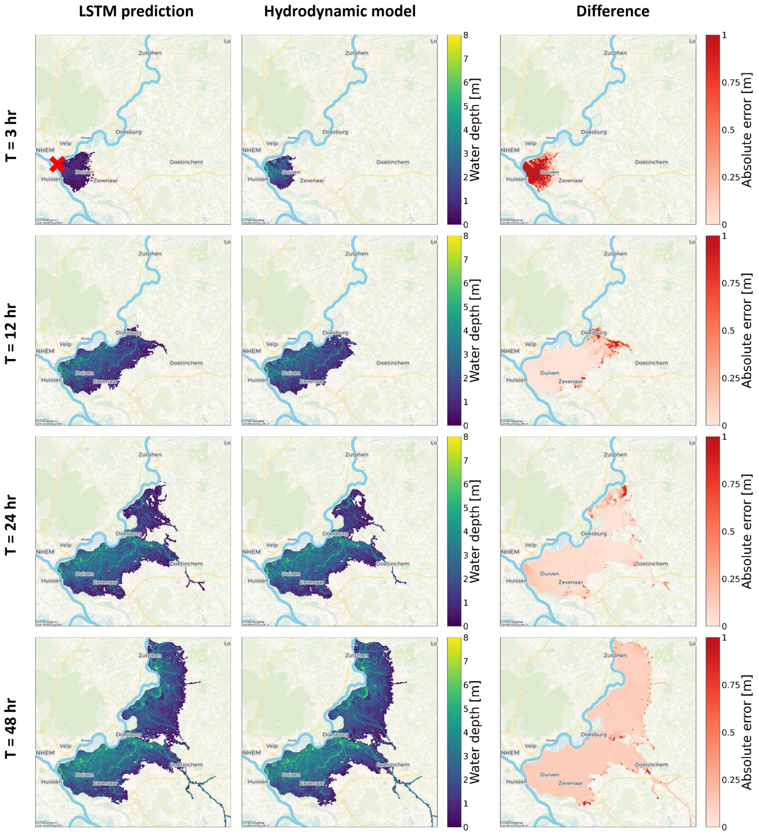
The water depth prediction of the LSTM is highly accurate in both inundation extent and water depths, when compared to the hydrodynamic model (Figure 5). Only during the first time step can a major difference in the water depths be observed between the two models. A possible cause lies in the nature of the LSTM memory cells, which require a time step to update their values appropriately. In this case, the first time step of predictions would utilize memory cells from the period before the flood, perhaps leading to the lower predicted water depths at the first time step after the breach. Then, the memory cells update to reflect the start of the flood, and starting from the second time step the water depth prediction becomes more accurate. Thus, modelling with a smaller time step can contribute to reducing the effect of this delay for a more accurate prediction, though the effect will likely still be present on the smaller inundation extent of the first time step.
The Mean Absolute Error (MAE) of all flooded grid cells and all time steps of this LSTM was 0.045 m, when tested on the unknown test data set. The average water depth of all these grid cells throughout these 15 simulations is 1.49 m in the hydrodynamic model, so the average water depth error is just 3% for these scenarios. The errors for the first two and four days after the breach are slightly higher, at 0.082 and 0.071 m, respectively. The Root Mean Square Error (RMSE) of all flooded grid cells and time steps shows the same behaviour as the MAE. For the 15 test flood events, the average RMSE is 0.13 m. The error is slightly higher at 0.17 and 0.19 m for the first two and four days after the breach, respectively. Overall, the RMSE values are higher than the MAE, which is caused by the large error in the first time step having a larger weight in the RMSE computation. Additionally, the MAE and RMSE are higher for shorter evaluation time frames due to the large error in the first time step, which contributes more to the MAE and RMSE when fewer time steps are evaluated.
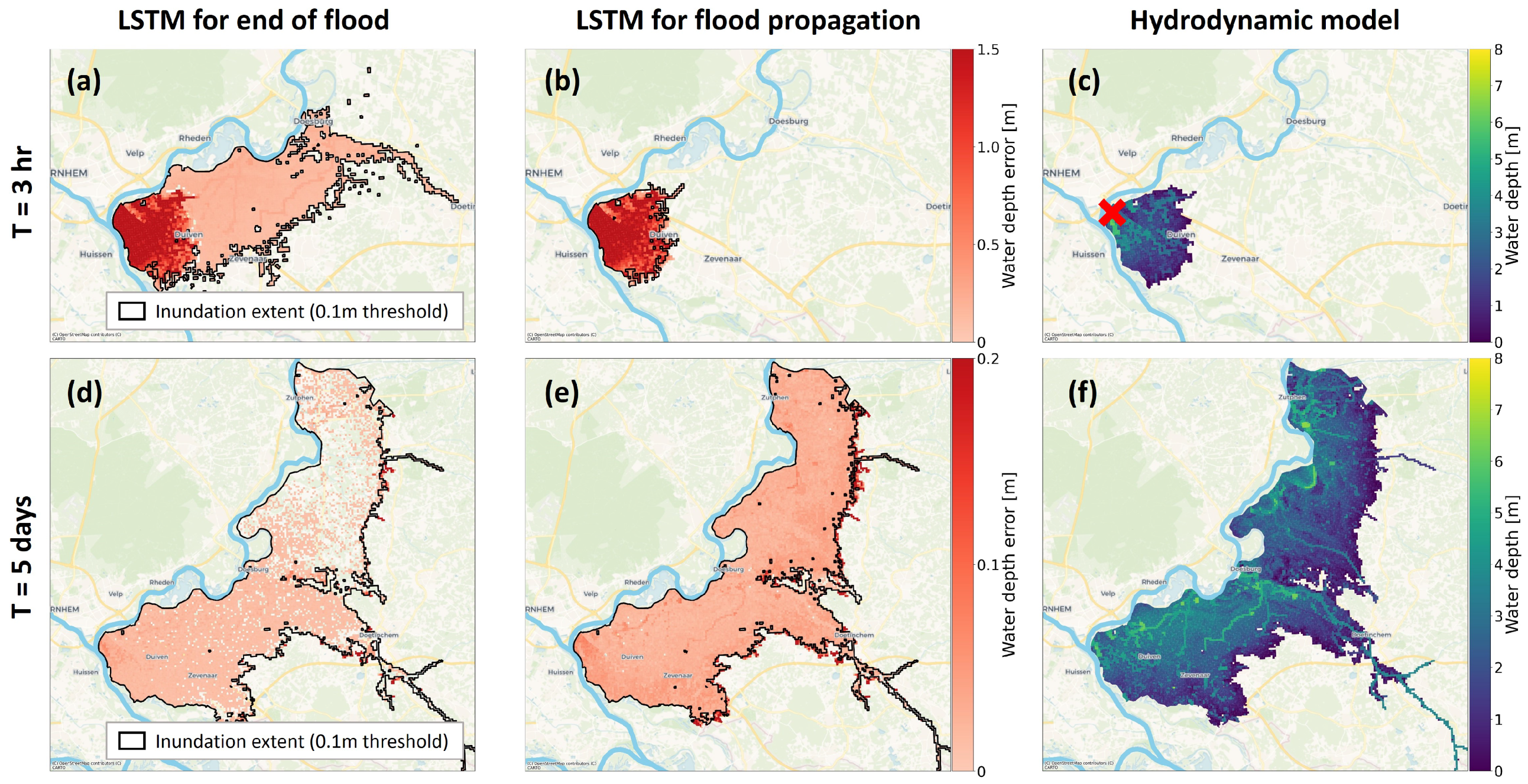
Out of all models trained and evaluated by the optimization algorithm, the LSTM of Figure 5 achieved the best MAE, RMSE and CSI during the first four to five days after the breach, in which the flood was propagating through the hinterland. However, it should be mentioned that a model with a slightly different combination of hyperparameters scored slightly better in terms of the MAE and RMSE for all time steps (Table 1). This other LSTM with an MAE/RMSE of 0.038/0.092 m across all time steps predicts an oversized flooded area for the first time step (Figure 6a), with small water depths compared to the flood propagation LSTM and the hydrodynamic model result (Figure 6b–c). Starting from 5 days after the breach to the end of the simulation, however, this other LSTM model performed slightly better across the complete area of flooded grid cells (Figure 6d compared to e and f). This compensates for the poorer performance during the flood propagation phase, resulting in a lower overall MAE and RMSE for all time steps. However, the propagation phase up until the maximum inundation extent is arguably the most important to predict accurately, as it allows analysis of flood arrival times and in the end a relevant planning of evacuation strategies. Therefore, the LSTM with the best MAE and RMSE scores during the flood propagation phase is considered the most suitable model out of the hyperparameter optimization. We discuss this phenomenon in Section 6.1.

5.2. LSTM Predictions

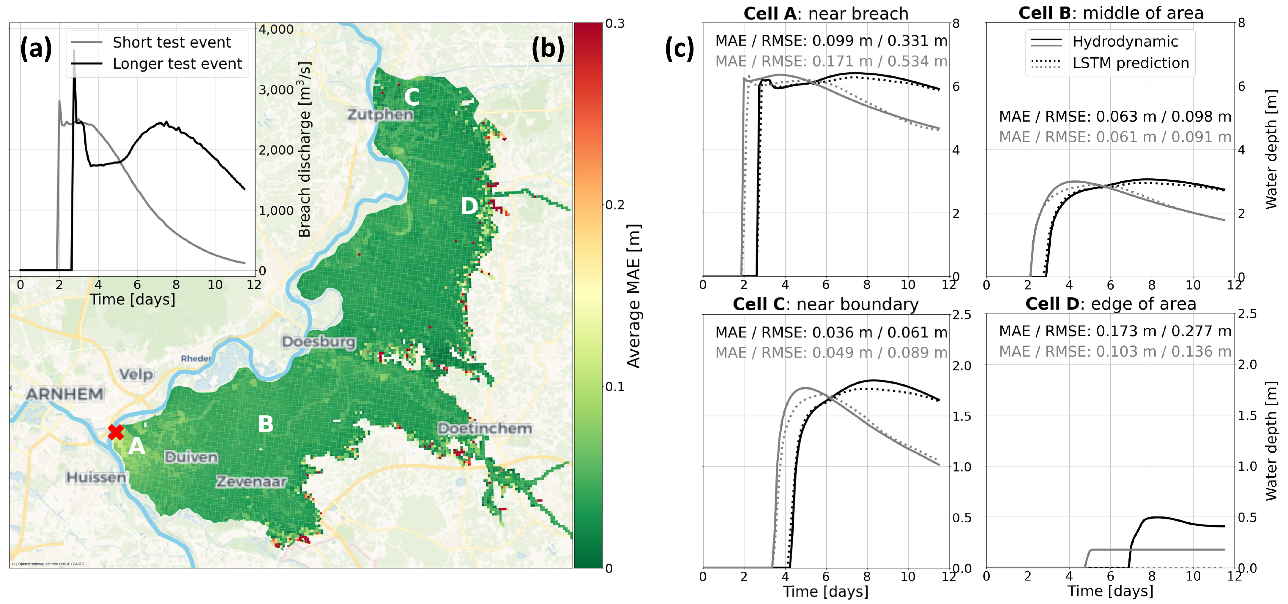
Evaluating the Mean Absolute Error (MAE) for the LSTM on the unseen testing data set, it becomes clear that the water depths were predicted accurately. Averaging the MAE across the 15 test flood scenarios, the LSTM scores low errors of less than 10 cm throughout most of the study area (Figure 7b). Near the dike breach, the LSTM has a slightly higher error of approximately 15 cm. This is caused by the apparent delay of one time step in the prediction of the LSTM compared to the hydrodynamic model which was discussed in Section 5.1.
Another striking observation in Figure 7b is the performance along the edges of the flood. As the flood water depths along this wet–dry border are generally quite small, it seems that the LSTM has difficulty learning when a particular scenario leads to flooding in a particular grid cell. This can be caused by these outer grid cells flooding only in the most severe flood scenarios; thus, the training data set contains few data points for these cells. However, the water depths here are generally small (between 0.1 and 0.5 m) and the width of this poorly predicted edge is at most 1 km. If the practical purpose of the LSTM would be to decide on evacuation measures, taking into account such a margin of error around the edges of the predicted flood would be wise regardless of the model accuracy.
The water depth prediction on single grid cells is shown to be accurate for both shorter and longer-lasting flood scenarios (Figure 7c). The figure shows the water depths decreasing much sooner for the shorter scenario than for the longer-lasting event, a behaviour which the LSTM can capture well. The delay in the first time step discussed in Section 5.1 is visible too, which causes an MAE of more than 10 cm and RMSE of more than 30 cm in cell A near the breach. In the middle of the study area (cell B) and near the northern boundary (cell C), the prediction by the LSTM is nearly identical to the hydrodynamic model water depths. The previously mentioned poorer performance in the edge region of the flooded area is also shown (cell D).
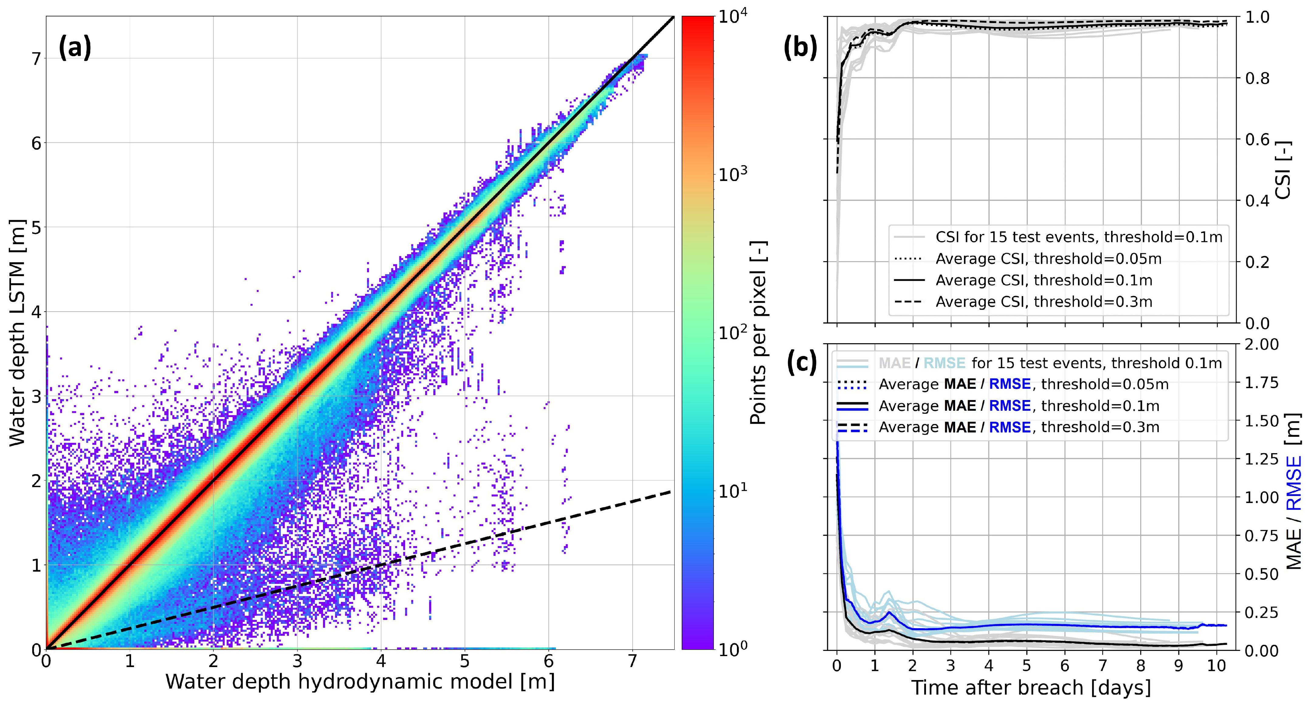
To visualize the LSTM prediction for every grid cell and time step in the 15 test flood events, a scatter density plot of the LSTM water depths against the hydrodynamic model water depths is shown in Figure 8. The majority of the data points are located along the solid black line that indicates perfect prediction. An interesting observation is the trail of points in a less steep slope along the dashed line, reflecting high hydrodynamic model water depths but low LSTM predictions. These points are the data of the first time step close to the breach, which were described in Section 5.1 as the delay of one time step between the LSTM and hydrodynamic model results.
The temporal variation of the MAE, RMSE and CSI for the 15 test flood events shown in Figure 8 indicates that the model performs accurately throughout the simulations. As the dike breaches, the performance indicators are less accurate compared to later in the flood. The MAE and RMSE start around 1.25 m for the first time step of the flood, which is due to the delay described in Section 5.1. They then quickly drop to around 0.1 m and lower for the rest of the simulation. The CSI starts at an average value of 0.6 for the first time step after the breach, increasing to 0.85 in the second time step. The average CSI reaches 0.95 one day after the breach and stays around 0.98 for the remainder of the simulations. The effect of different wet–dry thresholds is shown to be small, with different threshold values not leading to large changes in the average MAE, RMSE or CSI scores throughout the test flood events (Figure 8). Therefore, the LSTM consistently predicts the flood accurately with respect to the hydrodynamic model.

6. Discussion

In recent years, neural networks have mostly been applied to predicting flood water levels or discharges in rivers. In this study, for the first time, maps of water depths in time are predicted for large-scale overland flow after a dike breach using a single LSTM. The neural network has proven to be able to distinguish between the high and fast-increasing water levels close to the breach and the slower increase in water levels further away from the breach. The performance was also highly accurate for flood scenarios that were not present in the training data set.

6.1. Limitations and Improvements

In this study, the training data set created with the hydrodynamic model is considered the ground truth. This means that the accuracy of the LSTM can only be increased by improving the accuracy of the hydrodynamic model data. For example, the available hydrodynamic model data had a fixed output interval of 3 h, which was independent from the moment of breaching. As a result, the first output map after the breach of some scenarios contained the flood volume of only a short amount of time, while others contained 2.5 h of flood volume. This made the LSTM neural network perform less accurately compared to the hydrodynamic model in these scenarios. Additionally, the different breaching moments in these scenarios (discussed in Section 4.1 and shown in Figure 4) caused unrealistic behaviour in scenarios with late breaches. In these scenarios, the LSTM flooded a few grid cells near the breach just above the wet–dry threshold, while the input was still 0. A possible explanation is that the network has learned the usual moment of breaching so that for late-breach scenarios it already predicts a few cells with small water depths at that moment. When the breach does start and the input is no longer 0, the network recognizes this and starts to model the flood accurately. We ignored the outputs of the network while the input was still 0, since we were interested only in the flood propagation phase. However, for other authors to circumvent both these problems and obtain more robust machine learning models, we strongly recommend that the flood training scenarios start from the moment of breaching to ensure consistent timing frames.
A second point of attention is that in the optimized neural network, the number of neurons in the LSTM layer (928) was close to the maximum imposed during the Bayesian optimization (1024). This maximum was imposed due to the 6 GB memory limit on the NVIDIA GTX-1060 GPU available for the research. For further research, especially on hardware-limited devices, we recommended to look into a network setup that requires fewer neurons, to free up memory for larger or more detailed case studies. For example, only a selection of grid cells in the hinterland could be used for the neural network training, reducing the input and output size. Then, the output of the neural network could be post-processed using interpolation strategies, to compute the flood water depths in the entire study area. However, such a method could come at the cost of reduced accuracy.
Another recommendation is to define a loss function that is more specific to the modelled problem and desired outcome. For instance, the goal of the envisioned real-time flood forecasting system is to be able to aid in successful and timely evacuation. Thus, accurately predicting the flood propagation up to the maximum inundation extent is more important than the water depths after multiple days. In this study, we found that the Mean Absolute Error (MAE) can give varied conclusions on which model is best, depending on the time frame of evaluation (Section 5.1). As such, a more complex loss function combining water depth and flood extent could be developed that punishes the network more heavily for errors in the first days of the flood simulation up to the maximum inundation extent.

6.2. Application

Regarding the practicality of the LSTM developed in this study, the simulation time of the neural network is around 0.1 s, whereas the hydrodynamic model requires 6 to 10 h per simulated scenario on the available hardware. The near-instant simulation times allow for fast modelling during an emergency situation. The current model setup can handle varying outflow hydrographs as its boundary condition. These outflow hydrographs have to be quickly estimated in advance, possibly through the use of a 1D–0D river–hinterland model to limit the required computation in time-sensitive situations. With an envelope of possible outflow hydrographs, the neural network can be used to quickly evaluate each one of them to come to a prediction for the flood extent. This approach could take into account the uncertainty in factors such as final breach width and complicating aspects such as reduced/reversed breach outflow due to rising hinterland water levels. The output would then be a probabilistic inundation/depth map, instead of deterministic water depths for one scenario.
The main technical limitation for the application of the LSTM model in this study is that varying breach locations or changes in the hinterland were not considered. As such, the LSTM has no internal notion of location or water flow from cell to cell: it only trains each cell to respond in a particular way to an outflow hydrograph. This means that for a flood forecasting system using this approach, multiple of these LSTMs should be developed for each possible breach location. Gathering the training data would be very time-consuming and result in a large database of scenarios and corresponding flood maps. This database could be used for flood forecasting instead of the neural network, similar to how current emergency response is organized. Therefore, more research is needed into making neural networks less dependent on highly specific training data.
Finally, we would like to comment on bridging the gap between advances in machine learning and the application by practitioners. As discussed by Leskens et al. [6], decisions in flood disaster management are poorly supported by flood models, partly because the models lack speed and flexibility. Machine learning models could resolve this part of the issue and provide more scenario-based analyses to decision makers. However, machine learning models are typically viewed as black box models, so it is an open question how trust in these models can be gathered.
Some research fields have dedicated testing functions or data sets on which all new methods and models are benchmarked, which may help increase trust in machine learning models, too. For example, the famous MNIST data set of handwritten digits [40] is used to benchmark image classification models, with new techniques being evaluated on this data set. In flood modelling, we find only a limited culture of evaluating new techniques or models on benchmark case studies. An example is the hydrodynamic model benchmarking study conducted by Neelz and Pender [41], which has been used by Wijaya and Yang [42] to evaluate the performance of a cellular automata flood model. We follow the recommendation of Karim et al. [43] to publish the flood inundation data set used for this study, to hopefully contribute to an emerging culture of checks, benchmarks and building trust in robust machine learning techniques.

6.3. Future Research Directions

A promising research direction is to develop a generalized neural network that is able to model water flowing over an elevation map. This way, a model trained on a limited set of locations can be utilized in a wider variety of locations. Recently, Convolutional Neural Networks (CNNs) have been used more and more, because they can utilize spatial relationships between neighbouring cells on structured grids to extract and learn information [23,25]. Pianforini et al. [44] utilize a CNN layer to encode a flood map, followed by a Video Prediction Transformer Framework to predict the next time step of the flood, followed by a second CNN to decode the predicted data back to a flood map. Their approach can predict tens of time steps into the future with only a few past flood maps as input, instead of an incoming flood volume such as in this study.
Alternatively, the relatively new field of Graph Neural Networks (GNNs) uses graph theory, allowing the development of neural networks for irregularly structured data [45]. This overcomes limitations of structured grid cells, particularly in locations with sudden height increases or around raised structures. However, their applications have so far been mostly in the field of smaller-scale computational fluid dynamics (e.g., [46,47,48]). Recently, promising work by Bentivoglio et al. [49] has utilized GNNs to model water flow onto unseen computer-generated elevation maps of 40–160 km2, with a steady discharge of 50 m3/s. These techniques could help alleviate the problems caused by structured grids, as well as solve the problem of generalization for multiple breach locations. Their functioning in studies of large-scale overland flow on realistic topographies with realistic outflow hydrographs should be researched in more detail.
The next steps in the research field are to combine the efforts towards generalized breach locations with this research into varying and realistic outflow hydrographs. It is also important for the application of real-time flood forecasting in an emergency that a representative range of possible outflow hydrographs is evaluated for a possible breach. In this research, the constant breach width of 150 m resulted in a single outflow hydrograph per river discharge wave. However, many possible outflow hydrographs and inundation extents exist per river discharge wave, due to uncertainties in breach location, breaching mechanism and breach growth. This is why future work can be directed toward utilizing neural networks or other machine learning techniques to generate real-time flood probability maps, based on these various outflow hydrograph scenarios for incoming river discharge waves.

7. Conclusions

The objective of this study was to develop a neural network for predicting maps of hinterland water depths in time for large-scale overland flooding after a dike breach, using the outflow hydrograph as input. The chosen neural network, a Long Short-Term Memory (LSTM), has proven to be able to predict both the spatial and temporal flood behaviour both near to and far from a dike breach accurately, when compared to a hydrodynamic model considered as ground truth. For 15 unseen test scenarios not used for training, the Mean Absolute Error (MAE) in water depth was only 3% and the average Critical Success Index (CSI) reached up to 94%.
This LSTM setup offers flexibility in the outflow hydrograph used as forcing. Its main advantage is its high accuracy in this real case study of around 95% and its extremely short computation time in the order of milliseconds. This would allow for scenario analysis in case of an emergency situation and timely decision making on emergency measures such as evacuation. For wider application in a flood forecasting system, another important factor is the flexibility in dike breach location. If a future neural network setup such as a GNN or CNN can be generalized to predict for both various breach locations and varying breach discharges, there is large potential in the use of neural networks for providing an early and accurate indication of overland flow propagation in a real-time flood forecasting system.

Author Contributions

Conceptualization, L.S.B. and A.B.; methodology, L.S.B. and A.B.; software, L.S.B.; validation, L.S.B. and A.B.; formal analysis, L.S.B.; investigation, L.S.B.; resources, L.S.B.; data curation, L.S.B.; writing—original draft preparation, L.S.B.; writing—review and editing, L.S.B., A.B. and S.J.M.H.H.; visualization, L.S.B.; supervision, A.B. and S.J.M.H.H.; funding acquisition, S.J.M.H.H. All authors have read and agreed to the published version of the manuscript.

Funding

This research was funded by the Dutch Research Council’s (NWO) Simon Stevin Mastery grant received by Prof. Dr. Suzanne J.M.H. Hulscher.

Data Availability Statement

The data set used for training, as well as the code and final trained model, will be made available after publication at the 4TU.ResearchData repository under https://doi.org/10.4121/6fd289d8-ec0e-4dd9-94fd-4566783e9c3d [50]. For those interested in the HEC-RAS hydrodynamic model used to generate the training data, we refer to the Data Availability Statement in Bomers [27].

Conflicts of Interest

The authors declare no conflicts of interest.

References

  1. Schröter, K.; Barendrecht, M.; Bertola, M.; Ciullo, A.; da Costa, R.T.; Cumiskey, L.; Curran, A.; Diederen, D.; Farrag, M.; Holz, F.; et al. Large-scale flood risk assessment and management: Prospects of a systems approach. Water Secur. 2021, 14, 100109. [Google Scholar] [CrossRef]
  2. Mosavi, A.; Ozturk, P.; Chau, K.W. Flood prediction using machine learning models: Literature review. Water 2018, 10, 1536. [Google Scholar] [CrossRef]
  3. Alkema, D.; Middelkoop, H. The influence of floodplain compartmentalization on flood risk within the Rhine-Meuse delta. Nat. Hazards 2005, 36, 125–145. [Google Scholar] [CrossRef]
  4. Vorogushyn, S.; Merz, B.; Lindenschmidt, K.E.; Apel, H. A new methodology for flood hazard assessment considering dike breaches. Water Resour. Res. 2010, 46, 8541. [Google Scholar] [CrossRef]
  5. Chu, H.; Wu, W.; Wang, Q.J.; Nathan, R.; Wei, J. An ANN-based emulation modelling framework for flood inundation modelling: Application, challenges and future directions. Environ. Model. Softw. 2020, 124, 104587. [Google Scholar] [CrossRef]
  6. Leskens, J.G.; Brugnach, M.; Hoekstra, A.Y.; Schuurmans, W. Why are decisions in flood disaster management so poorly supported by information from flood models? Environ. Model. Softw. 2014, 53, 53–61. [Google Scholar] [CrossRef]
  7. Apel, H.; Thieken, A.H.; Merz, B.; Blöschl, G. Flood risk assessment and associated uncertainty. Nat. Hazards Earth Syst. Sci. 2004, 4, 295–308. [Google Scholar] [CrossRef]
  8. Bomers, A.; Schielen, R.M.J.; Hulscher, S.J.M.H. Consequences of dike breaches and dike overflow in a bifurcating river system. Nat. Hazards 2019, 97, 309–334. [Google Scholar] [CrossRef]
  9. D’Oria, M.; Maranzoni, A.; Mazzoleni, M. Probabilistic Assessment of Flood Hazard due to Levee Breaches Using Fragility Functions. Water Resour. Res. 2019, 55, 8740–8764. [Google Scholar] [CrossRef]
  10. Teng, J.; Jakeman, A.J.; Vaze, J.; Croke, B.F.W.; Dutta, D.; Kim, S. Flood inundation modelling: A review of methods, recent advances and uncertainty analysis. Environ. Model. Softw. 2017, 90, 201–216. [Google Scholar] [CrossRef]
  11. Bhola, P.K.; Leandro, J.; Disse, M. Framework for Offline Flood Inundation Forecasts for Two-Dimensional Hydrodynamic Models. Geosciences 2018, 8, 346. [Google Scholar] [CrossRef]
  12. Ferrari, A.; Dazzi, S.; Vacondio, R.; Mignosa, P. Enhancing the resilience to flooding induced by levee breaches in lowland areas: A methodology based on numerical modelling. Nat. Hazards Earth Syst. Sci. 2020, 20, 59–72. [Google Scholar] [CrossRef]
  13. Slomp, R.; Kolen, B.; Westera, H.; Verweij, J.; Riedstra, D. Interpreting the impact of flood forecasts by combining policy analysis studies and flood defence. E3S Web Conf. 2016, 7, 03006. [Google Scholar] [CrossRef]
  14. Dazzi, S.; Vacondio, R.; Mignosa, P.; Aureli, F. Assessment of pre-simulated scenarios as a non-structural measure for flood management in case of levee-breach inundations. Int. J. Disaster Risk Reduct. 2022, 74, 102926. [Google Scholar] [CrossRef]
  15. Vacondio, R.; Palù, A.D.; Mignosa, P. GPU-enhanced Finite Volume Shallow Water solver for fast flood simulations. Environ. Model. Softw. 2014, 57, 60–75. [Google Scholar] [CrossRef]
  16. Morales-Hernández, M.; Sharif, M.B.; Kalyanapu, A.; Ghafoor, S.K.; Dullo, T.T.; Gangrade, S.; Kao, S.C.; Norman, M.R.; Evans, K.J. TRITON: A Multi-GPU open source 2D hydrodynamic flood model. Environ. Model. Softw. 2021, 141, 105034. [Google Scholar] [CrossRef]
  17. Razavi, S.; Tolson, B.A.; Burn, D.H. Review of surrogate modeling in water resources. Water Resour. Res. 2012, 48, W07401. [Google Scholar] [CrossRef]
  18. McGrath, H.; Bourgon, J.F.; Proulx-Bourque, J.S.; Nastev, M.; Abo El Ezz, A. A comparison of simplified conceptual models for rapid web-based flood inundation mapping. Nat. Hazards 2018, 93, 905–920. [Google Scholar] [CrossRef]
  19. Campolo, M.; Andreussi, P.; Soldati, A. River flood forecasting with a neural network model. Water Resour. Res. 1999, 35, 1191–1197. [Google Scholar] [CrossRef]
  20. Minns, A.W.; Hall, M.J. Artificial neural networks as rainfall-runoff models. Hydrol. Sci. J. 1996, 41, 399–417. [Google Scholar] [CrossRef]
  21. Liu, Y.; Pender, G. A flood inundation modelling using v-support vector machine regression model. Eng. Appl. Artif. Intell. 2015, 46, 223–231. [Google Scholar] [CrossRef]
  22. Xie, S.; Wu, W.; Mooser, S.; Wang, Q.J.; Nathan, R.; Huang, Y. Artificial neural network based hybrid modeling approach for flood inundation modeling. J. Hydrol. 2021, 592, 125605. [Google Scholar] [CrossRef]
  23. Bentivoglio, R.; Isufi, E.; Jonkman, S.N.; Taormina, R. Deep Learning Methods for Flood Mapping: A Review of Existing Applications and Future Research Directions. Hydrol. Earth Syst. Sci. Discuss. 2022, 26, 4345–4378. [Google Scholar] [CrossRef]
  24. Staudemeyer, R.C.; Morris, E.R. Understanding LSTM—A tutorial into Long Short-Term Memory Recurrent Neural Networks. arXiv 2019, arXiv:1909.09586. [Google Scholar] [CrossRef]
  25. Kabir, S.; Patidar, S.; Xia, X.; Liang, Q.; Neal, J.; Pender, G. A deep convolutional neural network model for rapid prediction of fluvial flood inundation. J. Hydrol. 2020, 590, 125481. [Google Scholar] [CrossRef]
  26. Hosseiny, H. A deep learning model for predicting river flood depth and extent. Environ. Model. Softw. 2021, 145, 105186. [Google Scholar] [CrossRef]
  27. Bomers, A. Predicting Outflow Hydrographs of Potential Dike Breaches in a Bifurcating River System Using NARX Neural Networks. Hydrology 2021, 8, 87. [Google Scholar] [CrossRef]
  28. Le, X.H.; Ho, H.V.; Lee, G.; Jung, S. Application of Long Short-Term Memory (LSTM) Neural Network for Flood Forecasting. Water 2019, 11, 1387. [Google Scholar] [CrossRef]
  29. Yu, Y.; Si, X.; Hu, C.; Zhang, J. A Review of Recurrent Neural Networks: LSTM Cells and Network Architectures. Neural Comput. 2019, 31, 1235–1270. [Google Scholar] [CrossRef]
  30. Hochreiter, S.; Schmidhuber, J. Long Short-Term Memory. Neural Comput. 1997, 9, 1735–1780. [Google Scholar] [CrossRef]
  31. Sherstinsky, A. Fundamentals of Recurrent Neural Network (RNN) and Long Short-Term Memory (LSTM) network. Phys. D Nonlinear Phenom. 2020, 404, 132306. [Google Scholar] [CrossRef]
  32. Kao, I.F.; Liou, J.Y.; Lee, M.H.; Chang, F.J. Fusing stacked autoencoder and long short-term memory for regional multistep-ahead flood inundation forecasts. J. Hydrol. 2021, 598, 126371. [Google Scholar] [CrossRef]
  33. Kilsdonk, R.A.H.; Bomers, A.; Wijnberg, K.M. Predicting Urban Flooding Due to Extreme Precipitation Using a Long Short-Term Memory Neural Network. Hydrology 2022, 9, 105. [Google Scholar] [CrossRef]
  34. Karim, R. Animated RNN, LSTM and GRU: Recurrent Neural Network Cells in GIFs. 2018. Available online: https://towardsdatascience.com/animated-rnn-lstm-and-gru-ef124d06cf45 (accessed on 31 August 2024).
  35. Chollet, F. Keras. 2015. Available online: https://keras.io (accessed on 31 August 2024).
  36. Abadi, M.; Agarwal, A.; Barham, P.; Brevdo, E.; Chen, Z.; Citro, C.; Corrado, G.S.; Davis, A.; Dean, J.; Devin, M.; et al. TensorFlow: Large-Scale Machine Learning on Heterogeneous Systems. 2015. Available online: https://www.tensorflow.org/ (accessed on 31 August 2024).
  37. Pascanu, R.; Gulcehre, C.; Cho, K.; Bengio, Y. How to Construct Deep Recurrent Neural Networks. arXiv 2014, arXiv:1312.6026. [Google Scholar] [CrossRef]
  38. Rajaee, T.; Ebrahimi, H.; Nourani, V. A review of the artificial intelligence methods in groundwater level modeling. J. Hydrol. 2019, 572, 336–351. [Google Scholar] [CrossRef]
  39. Kingma, D.P.; Ba, J. Adam: A Method for Stochastic Optimization. arXiv 2017, arXiv:1412.6980. [Google Scholar]
  40. LeCun, Y.; Cortes, C.; Burges, C.J.C. The MNIST Database of Handwritten Digits. 1998. Available online: https://yann.lecun.com/exdb/mnist/ (accessed on 31 August 2024).
  41. Neelz, S.; Pender, G. Benchmarking the Latest Generation of 2D Hydraulic Modelling Packages; Technical Report; UK Environment Agency: Rotherham, UK, 2013.
  42. Wijaya, O.T.; Yang, T.H. A Novel Hybrid Approach Based on Cellular Automata and a Digital Elevation Model for Rapid Flood Assessment. Water 2021, 13, 1311. [Google Scholar] [CrossRef]
  43. Karim, F.; Armin, M.A.; Ahmedt-Aristizabal, D.; Tychsen-Smith, L.; Petersson, L. A Review of Hydrodynamic and Machine Learning Approaches for Flood Inundation Modeling. Water 2023, 15, 566. [Google Scholar] [CrossRef]
  44. Pianforini, M.; Dazzi, S.; Pilzer, A.; Vacondio, R. Real-time flood maps forecasting for dam-break scenarios with a transformer-based deep learning model. J. Hydrol. 2024, 635, 131169. [Google Scholar] [CrossRef]
  45. Scarselli, F.; Gori, M.; Tsoi, A.C.; Hagenbuchner, M.; Monfardini, G. The graph neural network model. IEEE Trans. Neural Netw. 2009, 20, 61–80. [Google Scholar] [CrossRef]
  46. Pfaff, T.; Fortunato, M.; Sanchez-Gonzalez, A.; Battaglia, P.W. Learning Mesh-Based Simulation with Graph Networks. arXiv 2020, arXiv:2010.03409. [Google Scholar] [CrossRef]
  47. Sanchez-Gonzalez, A.; Godwin, J.; Pfaff, T.; Ying, R.; Leskovec, J.; Battaglia, P.W. Learning to Simulate Complex Physics with Graph Networks. In Proceedings of the 37th International Conference on Machine Learning (ICML 2020), Virtual, 13–18 July 2020; PartF168147-11. pp. 8428–8437. [Google Scholar] [CrossRef]
  48. Liu, Q.; Zhu, W.; Jia, X.; Ma, F.; Gao, Y. Fluid Simulation System Based on Graph Neural Network. arXiv 2022, arXiv:2202.12619. [Google Scholar] [CrossRef]
  49. Bentivoglio, R.; Isufi, E.; Jonkman, S.N.; Taormina, R. Rapid spatio-temporal flood modelling via hydraulics-based graph neural networks. Hydrol. Earth Syst. Sci 2023, 27, 4227–4246. [Google Scholar] [CrossRef]
  50. Besseling, L.; Bomers, A.; Hulscher, S. Data Accompanying the Publication: Predicting Flood Inundation after a Dike Breach Using a Long Short-Term Memory (LSTM) Neural Network. 4TU.ResearchData. 2024. Available online: https://doi.org/10.4121/6fd289d8-ec0e-4dd9-94fd-4566783e9c3d (accessed on 31 August 2024).
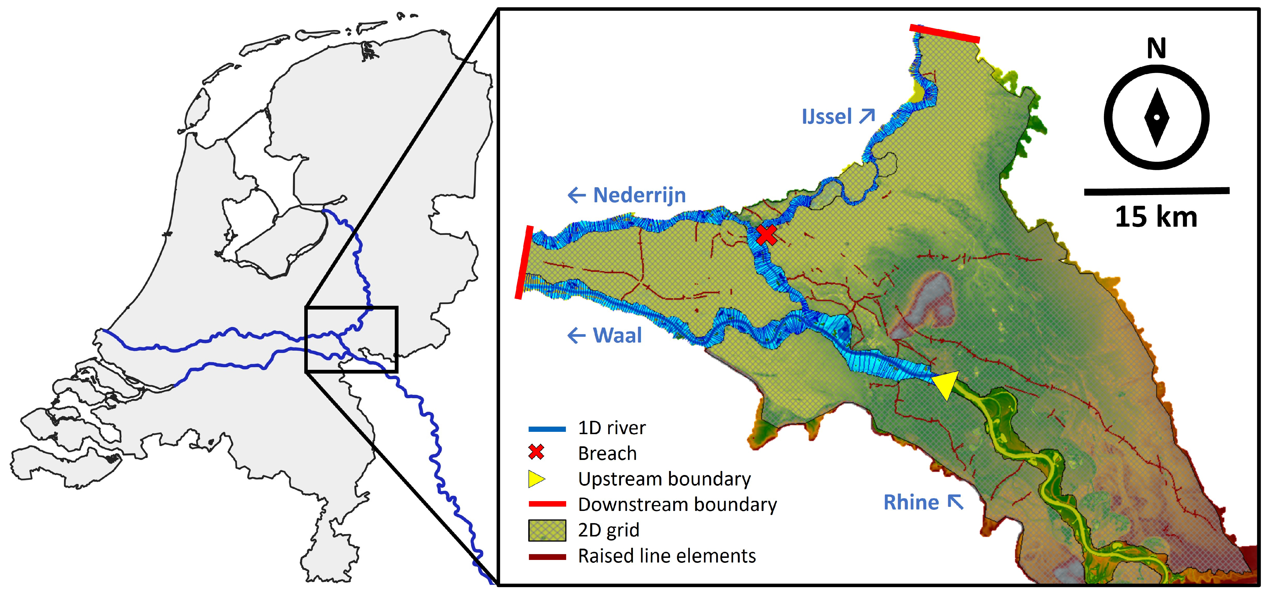
Figure 2. The study area of the Rhine river entering the Netherlands and bifurcating, and its representation in the 1D–2D hydrodynamic model of Bomers [27].
Hydrology 11 00152 g002
Figure 3. (a) Examples of river discharge waves at the boundary that lead to a breach downstream. The breach at the IJssel breach location occurs when the discharge in the Rhine reaches around 16,000 m3/s, marked with x on the three shown discharge waves. (b) The overland flow patterns computed by the hydrodynamic model of Bomers [27] during the black river discharge scenario of panel A at various times after the breach. Starting from the breach (at the red X) and spreading towards the north-east, the largest inundation extent is reached about 48 h after the breach.
Hydrology 11 00152 g003
Figure 4. The variability of the data set from Bomers [27]. (a) The input breach outflow hydrograph scenarios used for training and testing, with the hydrographs leading to the maximum and minimum inundation extents shown in blue and red, respectively. Figure 3a shows the corresponding river discharge at the upstream boundary in blue and red. (b) Map of the maximum and minimum inundation extents of the flood scenarios, and the difference in water depth between them per grid cell. Breach location indicated with a red X. (c) The water depths at locations A, B and C of panel B for all scenarios, with the max and min inundation scenarios indicated in blue and red, respectively.
Hydrology 11 00152 g004
Figure 5. Water depth predictions of LSTM model compared to hydrodynamic model for four time steps in the simulation of 1 of the 15 test flood events. Breach indicated with a red X.
Hydrology 11 00152 g005
Figure 6. Water depth prediction error of two LSTM models compared to the hydrodynamic model for a test data set flood. (ac) During the flood propagation phase (shown with the first time step after the breach), the end-of-flood LSTM model is less accurate than the LSTM model for flood propagation compared to the hydrodynamic model. (df) After 5 days, the end-of-flood LSTM model is more accurate than the flood propagation LSTM model compared to the hydrodynamic model. Breach indicated with a red X.
Hydrology 11 00152 g006
Figure 7. Results for the Mean Absolute Error (MAE) for the test flood events. (b) A map of spatial variation in total MAE per grid cell, averaging all time steps and all 15 test flood events. Breach indicated with a red X. (a) Outflow hydrographs of two specific test flood events, one with quickly diminishing breach outflow and one with longer continuation of the flood event. (c) The water depths in grid cells A–D of panel B for the short and long test flood events show that the LSTM is able to capture the difference in flood behaviour.
Hydrology 11 00152 g007
Figure 8. (a) A scatter plot of LSTM prediction against hydrodynamic model water depths for all grid cells and time steps during the 15 test flood events. Most of the 48 million data points are along the 1:1 solid line of perfect prediction, while only a few are scattered around. Some points concentrate along a less steep dashed line, which corresponds to the first time step delay between the LSTM and hydrodynamic model results. (b,c) The temporal variation of CSI and MAE/RMSE, averaged over all flooded grid cells for different wet–dry thresholds.
Hydrology 11 00152 g008
Table 1. Average MAEs, RMSEs and CSIs of all test flood events, for various evaluation time frames for two LSTM models: the LSTM model with the lowest overall MAE and RMSE and the LSTM with the lowest MAE and RMSE during the flood propagation phase. The best model per evaluation time frame indicated in bold.
MAE [m]RMSE [m]CSI [-]
Time after Breach [days]: 2 4 6 All 2 4 6 All 2 4 6 All
LSTM for end of flood0.140.0780.0570.0380.270.180.140.0920.810.890.920.94
LSTM for flood propagation0.0820.0710.0670.0450.190.170.170.130.910.940.950.94
Disclaimer/Publisher’s Note: The statements, opinions and data contained in all publications are solely those of the individual author(s) and contributor(s) and not of MDPI and/or the editor(s). MDPI and/or the editor(s) disclaim responsibility for any injury to people or property resulting from any ideas, methods, instructions or products referred to in the content.