Article

Machine Learning Model for River Discharge Forecast: A Case Study of the Ottawa River in Canada

Department of Building, Civil and Environmental Engineering, Concordia University, 1455 de Maisonneuve Boulevard West, Montreal, QC H3G 1M8, Canada
*
Author to whom correspondence should be addressed.
Hydrology 2024, 11(9), 151; https://doi.org/10.3390/hydrology11090151
Submission received: 15 August 2024 / Revised: 30 August 2024 / Accepted: 10 September 2024 / Published: 12 September 2024
(This article belongs to the Section Water Resources and Risk Management)

Abstract

:
River discharge is an essential input to hydrosystem projects. This paper aimed to modify the group method of data handling (GMDH) to create a new artificial intelligent forecast model (abbreviated as MGMDH) for predicting discharges at river cross-sections (CSs). The basic idea was to optimise the weights for selected hydrometric and meteorological predictors. One novelty of this study was that MGMDH could take the discharge observed from a neighbouring CS as a predictor when observations from the CS of interest had ceased. Another novelty was that MGMDH could include meteorological parameters as extra predictors. The model was validated using data from natural rivers. For given lead times, MGMDH automatically determined the best forecast equations, consistent with physical river hydraulics laws. This automation minimised computing time while improving accuracy. The model gave reliable forecasts, with a coefficient of determination greater than 0.978. For lead times close to the advection time from upstream to the CS of interest, the forecast had the highest reliability. MGMDH results compared well with some other machine learning models, like neural networks and the adaptive structure of the group method of data handling. It has potential applications for efficiently forecasting discharge and offers a tool to support flood management.

1. Introduction

River floods are a major global concern, causing substantial human and economic losses [1]. Historically, these events have devastated communities, with floods in 2016 alone affecting 74 million people, resulting in 4720 deaths and USD 57 billion in damages [2]. The impact of river floods can become more severe due to climate change, which has reportedly increased the frequency and intensity of floods [3,4,5,6,7,8,9,10]. Some regions in Canada are particularly vulnerable, with 100-year return floods potentially becoming 10- to 60-year events [3]. In the U.S., floods caused an average of 95 fatalities annually from 2009 to 2018 and USD 4.6 billion in damages per major event between 1980 and 2019 [7]. These statistics underscore an urgent need for effective flood management and adaptation strategies.
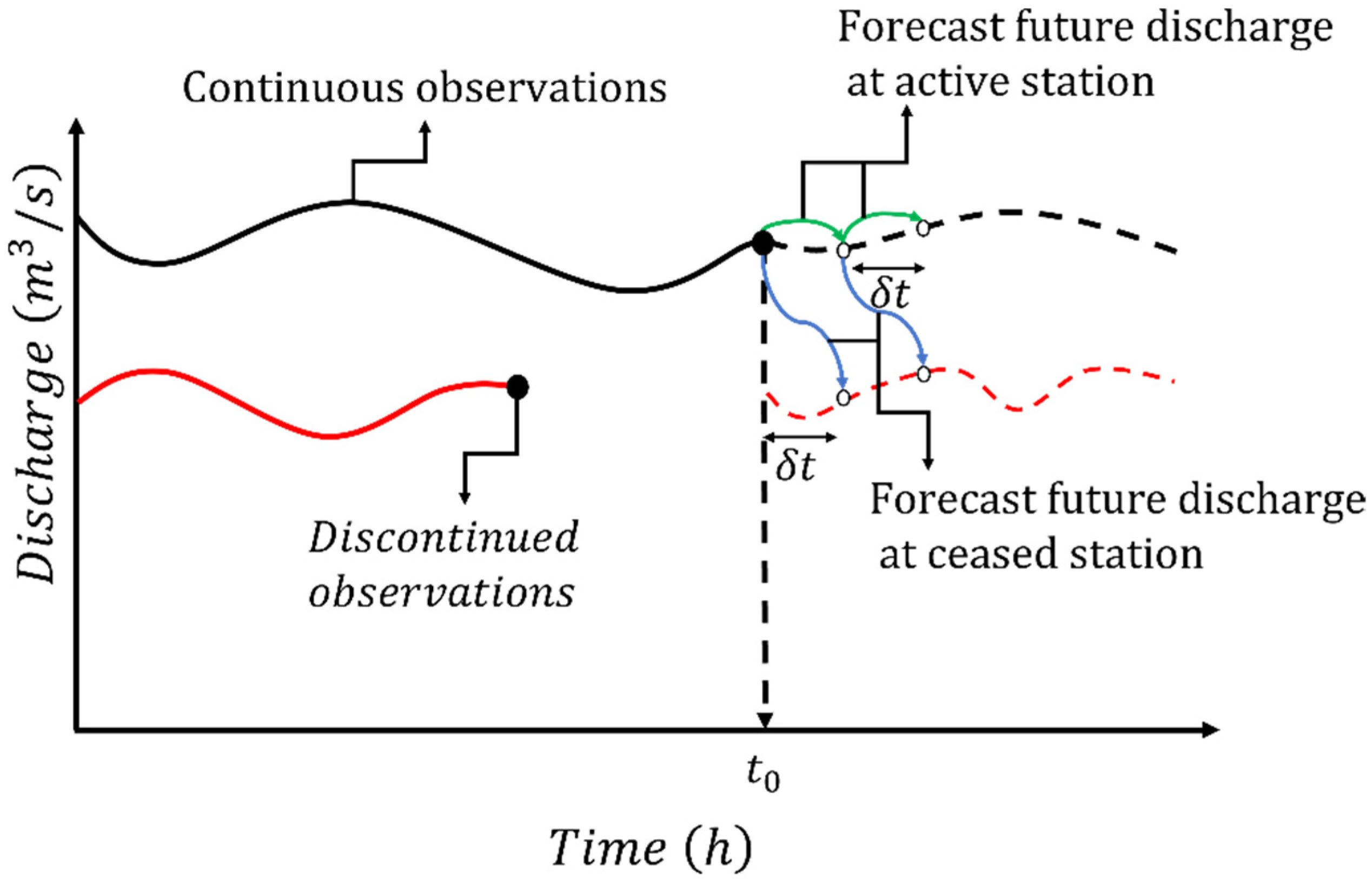
Floods occur when river discharge, q, exceeds a certain bankfull threshold. Thus, it is crucial to be able to predict discharge in real-time for the coming hours to provide early warning of floods, plan evacuation activities and structural measures, and prepare for flood hazards [11,12]. In order to improve the predictions about how q will change over the coming hours, the current initial value of q should be known, e.g., from real-time observations (Figure 1). However, in reality, continuous real-time observations from the river cross-section (CS) of interest may not be available, as schematically illustrated in Figure 2.
Extensive efforts have been made to predict river discharge using MLMs, including the widely used artificial neural network (ANN) [13,14] and long short-term memory (LSTM) [15,16,17,18,19,20]. Both ANN and LSTM capitalise on their data-driven capabilities. The ANN is known for its good learning capability, noise immunity, and generalisability, and has proven effective in hydrological applications [21]. For instance, Ekwueme (2024) [14] effectively predicted discharge in five rivers by optimising the neuron count in a three-layer ANN, utilising meteorological data as inputs. LSTM networks have the ability to capture long-term dependencies and have shown remarkable success in hydrological forecasting. Liu et al. (2021) [15] applied an LSTM-based rolling forecast to predict short-term water levels, adjusting for varying observation intervals and forecast times. Similarly, Kao et al. (2024) [20] employed an LSTM-based encoder–decoder model for multi-step-ahead forecasting of reservoir inflows, accurately predicting up to six hours ahead based on preceding hourly inflow and rainfall data. There are also studies (e.g., Skoulikaris and Nagkoulis (2024) [22]) that use genetic algorithms for enhanced rainfall distributions for accurate simulations of flood events.
The drawbacks of the previous studies include: (a) MLMs are black-box models, making it difficult to interpret results; (b) they require large amounts of input data and incur high computing costs; (c) they encounter challenges in pre-processing datasets and automatically selecting predictors; and (d) some of the MLMs have used only precipitation and temperature as predictors in the meteorological module. Most of the previous studies have overlooked the need for discharge forecasts on hourly time scales, which are arguably the most relevant for early warning and preparedness during flood seasons.
Previous studies have mostly focused on daily and multiple-day forecasting of streamflow, which is useful for water management. Girihagama et al. (2022) [23] developed a real-time forecasting model considering multiple lead times, ranging from one to five days, using LSTM models. Similarly, Alizadeh et al. (2021) [24] found that their novel LSTM model outperformed others in low, medium, and high flow ranges for one- to seven-day ahead forecasts across various basins. Adnan et al. (2019) [25] used hydro-climatic data to predict and estimate daily streamflow. Cheng et al. (2020) [26] assessed forecast performance for lead times from one to twenty days, noting decreased accuracy with increased lead time. However, limited studies have focused on accurate real-time hourly discharge forecasting, which is equally important for effective water management.
Recently, GMDH techniques have successfully been applied to hydrology problems [27,28,29,30,31]. Souza et al. (2022) [32] applied particle swarm optimisation to fine-tune the training–testing split in the GMDH model for predicting river flow one day in advance. Elkurdy et al. (2022) [33] employed the generalized structure group method of data handling for short-term flow forecasting, using discharge data from the previous two to five timesteps. Their models demonstrated acceptable accuracy, achieving an R2 value of 0.90 for predictions up to 17 h ahead. Letessier et al. (2023) [30] modified the GMDH techniques by introducing an adaptive structure for the prediction of daily river discharge and incorporating the 2nd- and 3rd-order polynomial functions to capture nonlinearity. These studies have overlooked the linear relationship which can effectively reduce forecast errors in some cases.
The objectives of this study are to:
  • Incorporate observational data of q into a machine learning model (MLM) for expeditious and accurate forecasting. High efficiency is crucial for early warning during flood seasons, hazard preparedness, and evacuation activities.
  • Modify the group method of data handling (GMDH) and demonstrate the applicability of the modified GMDH (MGMDH) to natural river sites.
The novelty of this study lies in treating both continuous and discontinued observation cases. The significance of this work is as follows:
  • In the case of discontinued observations, MGMDH techniques allow one to digitally reactivate a ceased station, which is much less expensive than resuming its field operations. To the best of our knowledge, this cost-effective alternative is new.
  • In both cases, the prediction q ^ for coming hours can give necessary boundary conditions to support detailed hydraulics modelling of a river section, e.g., the section bounded by CSU and CSD in Figure 3, using HEC-RAS [34,35], MIKE11 [36,37], SWAT [38], or TELEMAC [39].
In this study, MGMDH techniques offer interpretable polynomial regression functions and work well even if the amounts of data available are small. The computations are efficient, with minimal risks of overfitting.
In the following section, the methodologies are described. Then, applications of the methodologies to two hydrometric stations in the Ottawa River (Figure 1), Ontario, Canada, are presented, and improvements to the techniques are demonstrated. This is followed by a discussion of the forecast results before conclusions drawn. This study assesses the influence of integrating meteorological data on the accuracy of the results.

2. Methods

2.1. River Discharge Forecast Model

Let q ^ denote the discharge at a cross-section (CS) of interest in a river channel (Figure 3, CSD), t o denote the current time, and δ t denote a time increment (in hours). The value of q ^ at time t = t o + δ t is forecasted using a Kolmogorov–Gabor polynomial of the form
q ^ = f x 1 , x n , t = w 0 + i = 1 n w i x i + i = 1 n j = i n w i j x i x j + i = 1 n i = i n k = j n w i j k x i x j x k +
where x 1 , x 2 , , x n are n independent variables or predictors evaluated at time t o , and w i , w i j , and w i j k are the coefficients or weights that reflect the influence of the terms in the model equation. In Equation (1), the first term w 0 is the bias of the model, the second term expresses a linear dependence of discharge on x i   ( i = 1 , 2 , , n ) , and the remaining terms are a non-linear dependence. Here, t is considered as a parameter.
The idea is to use a layered and iterative approach to determine the coefficients in order to capture and anticipate the intricate interactions and patterns that exist between the discharge and the predictors. A large number of different models for q ^ may exist, each corresponding to a set of different values for the coefficients. For certain predictors to be included in Equation (1), observed values must be available. On the basis of river hydraulics and river basin hydrology, examples of potential predictors include: (1) q U , (2) η D , (3) river basin precipitation P, and (4) river basin air temperature T. The approach to discharge forecast (Equation (1)) is conceptually simple.
Nevertheless, combinations of the potential predictors lead to a large number of models or different forms of Equation (1). It is challenging and time-consuming to discern the most influential predictors and further quantify their weights. Suitable predictors can be selected with the help of fundamental physical laws that govern river flow. For example, the principle of mass conservation implies a link of q ^ (or q D ) to q U , while the energy principle leads to a relationship between η U and η D . Unlike models based on physical laws, the discharge forecast model (Equation (1)) does not require input data such as riverbed geometries between CDU and CSD and uncertain bed friction parameters. Such input data may not be available and is expensive to obtain.

2.2. Model Training

This study dealt with the challenge by adopting a modified version of the group method of data handling from the original work of Ivakhnenko (1971) [40], because of its advantage over other machine learning techniques. This advantage lies in the self-organising approach to mathematical modelling, allowing for a range of potential models during training, simultaneously exploring multiple model structures, and automatically selecting the most suitable one. This study used a modified version of this method. Suitability was assessed using the least squares method, with the normalised mean squared error (NMSE), ε , as the objective function given by
ε = m 1 l = 1 m ( q l q ^ l ) 2 V a r ( q l )
where q 1 , q 2 , , q m are a dataset for model training, which consists of m samples of discharges observed from CSD (Figure 3), and q ^ 1 , q ^ 2 , , q ^ m are the corresponding discharges predicted from Equation (1). The error was normalised by the sample variance of the actual discharges, using it as an unbiased estimator [41].
The objective was to minimise ε through the refinement of models. The refinement started with a simple model (e.g., a sole predictor, Equation (1)) and progressed to increasingly complex models (i.e., multiple predictors) only when it improved ε . This approach helps achieve a balance between model sophistication and prediction quality. On the other hand, data overfitting needs to be avoided because the resultant model may lose generality. To prevent overfitting, the dataset q 1 , q 2 , , q m was divided into subsamples using a v-fold method with 5 folds for model training. For more details about the v-fold method, refer to Hipni et al. (2013) [42] and Modaresi and Araghinejad (2014) [43].
It is preferred to encompass linear, 2nd-order, and 3rd-order polynomial functions for short-term (sub-diurnal) forecasts of river discharges. Such polynomial functions allow efficient computations. Such forecasts are crucial for issuing timely warnings of river flooding hazards at downstream locations and enabling nearby riverine communities to act swiftly. This is particularly important for locations where monitoring hydrometric stations have ceased operations.

2.3. Model Testing

Following the model training mentioned above, the model in question was tested using a dataset of M samples of observed discharges: q m + 1 , q m + 2 , , q m + M from CSD (Figure 3). This testing quantifies the model performance.

2.4. Model Validation (Data Comparison)

Further model performance validation was performed based on five statistical indicators:
  • The coefficient of determination, R 2 , given by
    R 2 = 1 l = m + 1 m + M ( q l q ^ l ) 2 l = m + 1 m + M ( q q ¯ ) 2
    where q ¯ is the mean value of q m + 1 , q m + 2 , , q m + M . R 2 reveals the proportion of the variance of the discharges predictable from x 1 , x 2 , , x n (Equation (1)) and thus the goodness of fit. The larger the R 2 value, the better the fit. R 2 has the same value as the Nash–Sutcliffe efficiency coefficient widely used in the field of hydrology.
  • The normalised root mean square error, ε ~ , given by
    ε ~ = 1 q ¯ 1 M l = m + 1 m + M ( q i q ^ l ) 2
    This is the average model error relative to the range of discharges and allows for cross-dataset comparisons, independent of the magnitude, and is more accurate across diverse datasets. A lower ε ~ value means a smaller average deviation of q ^ from actual values.
  • Mean absolute relative error, ε a , given by
    ε a = 1 M l = 1 M q l q ^ l q l
    This is the average percentage error. The lower the ε a value, the more accurate the model.
  • Akaike information criteria (AIC), c, expressed as
    c = M log l = m + 1 m + M ( q l q ^ l ) 2 M + 2 n n + 1 M n 1
    which is crucial to finding a balance between model accuracy and complexity. The goal is to seek a lower c value, meaning that the model adeptly captures the underlying patterns while prioritising simplicity and avoiding overfitting.
  • The term reliability determines whether or not the model in question achieves an acceptable level of performance [44]. It ascertains the model’s consistency and reproducibility of observations. Reliability is given by
    R e = 100 M l = 1 M R l
    R l = 1 ,   q l q ^ l / q l < α 0 ,   q l q ^ l / q l α
    where α is an allowable relative error. Following Ebtehaj and Bonakdari (2022) [44] and Letessier et al. (2023) [30], the model testing used α = 0.01 , 0.02 , 0.05 , 0.1 , 0.15 , 0.2 . The idea is to test the extent to which the model is reliable, valid, and well-suited for the intended analysis.
  • Dimitriadis et al. (2016) [45] introduced two benchmark solutions:
    F B 1 = 1 l = M m + M q ¯ q ^ l 2 l = M m + M q ¯ q 2
    F B 2 = 1 l = M m + M q t 0 q ^ l 2 l = M m + M q ¯ q 2
    where q t 0 is the discharge at CSD at time t 0 . If F B 1 0 and F B 2 0 , the prediction of discharge for the lead time (or time window) in question is considered to be acceptable.
When observations from a neighbouring station are used, this station and the station in question should be from a homogeneous system, meaning temporal consistency in climatic, topographic, and hydraulic conditions. The two stations in a river stream need not be in the same reach (Figure 3).
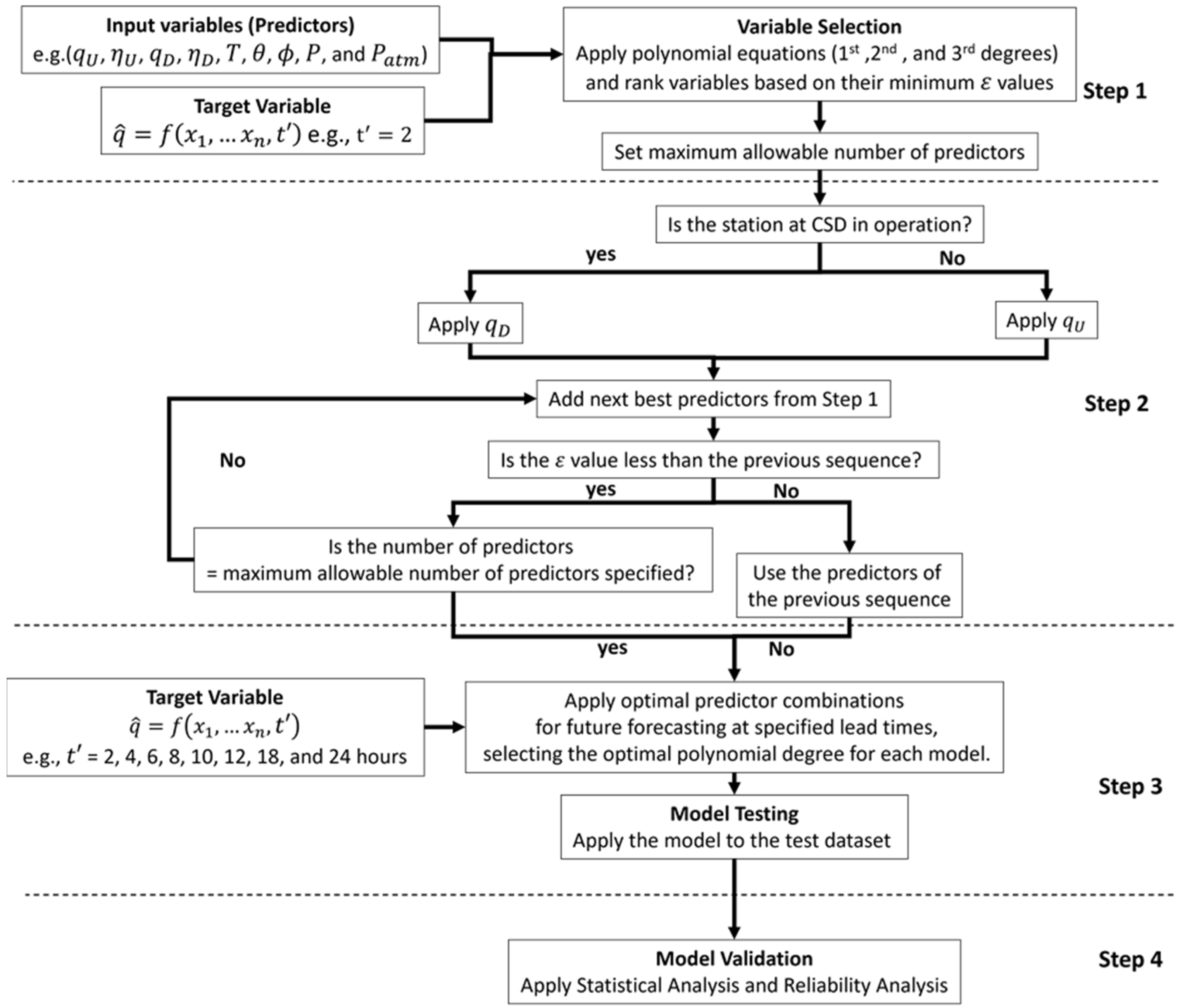
The flowchart of the MGMDH model data-driven framework is illustrated in Figure 4. The methodology began with a sole predictor analysis, where each predictor was evaluated individually, ranked, and sorted based on its normalised mean squared error (NMSE). The model then advanced by incorporating additional data, considering the status of the hydrometric station—either active (including its predictors) or ceased (using predictors from another station within the same river, along with meteorological data). The model systematically combined the best predictors, with the MGMDH sequentially adding predictors only if they enhanced prediction accuracy. This process continued until the hyperparameter for the maximum number of predictors was reached. The methodology was then applied to develop unique models for each lead time, with performance metrics used to validate the final models.
In summary, the GMDH is a self-organising modelling approach that creates complex polynomial models by selecting and combining functions of input variables through a multi-layered, iterative process. The original GMDH model generates either linear or quadratic equations by adjusting weights to predict the output variable (discharge) from the given input variables (predictors). The MGMDH proposed in this paper allows for 1st, 2nd, and 3rd degree polynomials.

3. Results

3.1. Predictors for Discharge Forecast

The Ottawa River was used as an example to demonstrate the methods (Figure 4) for discharge forecast (Equation (1)). The river CS of interest (WSC station ID: 02KF005) is located at 45°21′04″ N, 75°49′35″ W, marked as CSD in Figure 1. This paper explored the novel idea of replacing q D with available discharge q U from a neighbouring CS of the river, using a transparent MLM. This idea involves spatiotemporal extrapolations. The neighbouring CS (WSC Station ID: 02KF009) is located at 45°28′30″ N, 76°14′21″ W, at a distance of about δ x 43 km upstream from CSD. This neighbouring CS is marked as CSU in Figure 1.
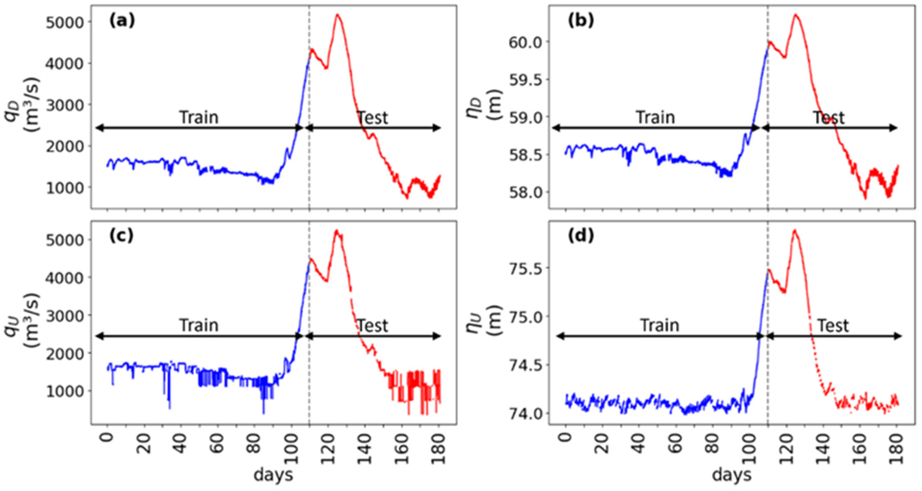
Time series of observed hourly averaged discharge q D and water level η D (Figure 5a,b) from CSD, and q U and water level η U (Figure 5c,d) from CSU were retrieved from the WSC database. The data showed seasonal variations and peak values from April to May (snow melting period). Here, 60% of q D data points (first 110 days) were used to train the model or determine the coefficients in Equation (1), while the remaining 40% (last 70 days) were used to test the model or assess the accuracy of the resulting polynomial functions. This split of percentages is acceptable.
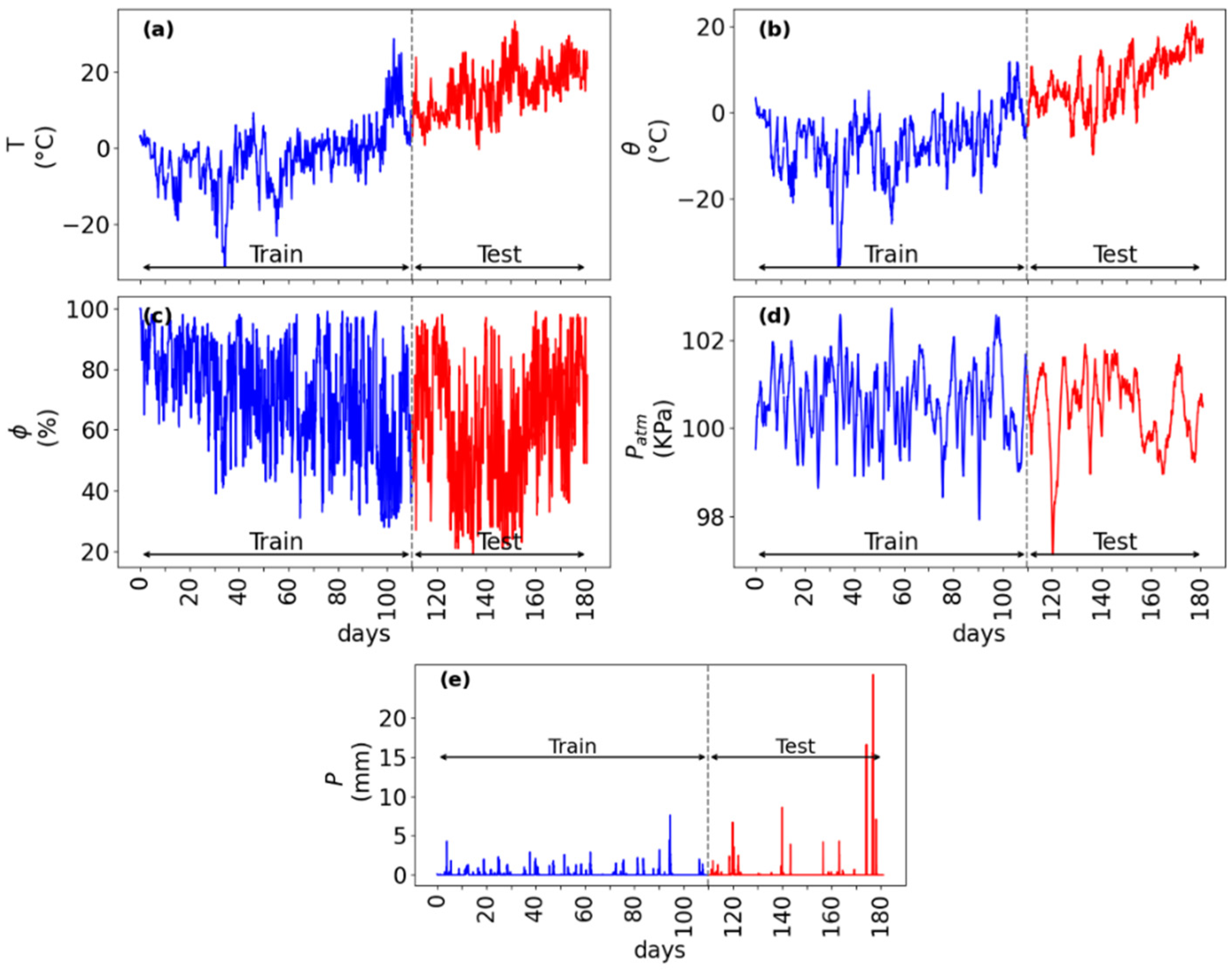
Watershed behaviour, and hence river discharge, may be influenced by air temperature, T , dew point temperature, θ , relative humidity, ϕ , precipitation, P , and atmospheric pressure, P a t m . Observations of these variables for the Ottawa River Basin are available (Figure 6). In summary, this study assessed a total of nine predictors (Table 1) for discharge (at CSD) forecast.
The magnitudes of q D differed significantly between the training dataset and the testing dataset. The former ranged from 704 to 5170 m3/s, with a standard deviation of 488 m3/s, whereas the latter varied from 1050 to 4120 m3/s, with a standard deviation of 1457 m3/s. It is a great challenge for an artificial intelligence model to capture the large variations in discharge present inf the testing dataset. Such varied discharge conditions serve the purpose of testing the model’s adaptability well.

3.2. Best Sole Predictor for Discharge Forecast

Among the nine predictors (Table 1), which is the best sole predictor for forecasting q ^ ? Step 1 of the methods (Figure 4) ranked them as follows. Take q U as an example. Training the model (Equation (1)) using 60% of q U data points (Figure 5c) produced polynomial functions for the given lead times. Let the lead time δ t be 2 h. The 1st, 2nd, and 3rd degree polynomial functions (Equation (1) of specific forms) were determined as
q ^ = f x 1 ,   t = f q U , 2 = w 0 + w 1 q U
q ^ = f x 1 ,   t = f q U , 2 = w 0 + w 1 q U + w 11 q U 2
q ^ = f x 1 ,   t = f q U , 2 = w 0 + w 1 q U + w 11 q U 2 + w 111 q U 3
where w 0 = 129.84 and w 1 = 0.91 in Equation (11); w 0 = 382.47 , w 1 = 0.67 and w 11 = 5.10 × 10 5 in Equation (12); and w 0 = 1.18 , w 1 = 5.71 , w 11 = 6.40 , and w 111 = 8.28 in Equation (13), as determined using the training data points (Figure 5c). For discharge prediction, the predictor q U in Equations (11)–(13) used input values from the training data points (Figure 5c). The reason for using training (as opposed to test) data points was due to the stage of model development. It is understood that the polynomial functions have coefficients having different values (not listed for conciseness) for different lead times (e.g., δ t = 4 , 8 and 18 h).
For δ t = 2 h, values of q ^ were predicted using the 1st degree polynomial function (Equation (11)). A comparison of these values with the training data points in Figure 5a showed a small NMSE ε = 0.002 (Equation (2); Table 1), indicating that Equation (11) was accurate. The 2nd degree polynomial function (Equation (12)) was acceptable, with a small ε (Table 1). The 3rd degree polynomial function (Equation (13)) was less accurate (Table 1). The forecast model given in Equation (11) was ranked the best among Equations (11)–(13).
For all nine predictors (Table 1), the same calculation procedures were implemented automatically using a Python script (without run-time manual control). Table 1 lists the ranking of the predictors as sole predictors for discharge forecast q ^ (Equation (1)), along with values of ε for δ t = 2 h. The conclusion was that the best four sole predictors were q D , η D , q U , and η U (Table 1). Will the various combinations of them as dual or triple predictors improve the accuracy of discharge forecast q ^ ? Step 2 of the methods (Figure 4) addressed this question. Note that the inclusion of only the best four predictors was not a limitation. In fact, MGMDH sequentially adds predictors if the addition improves the accuracy of q ^ (Equation (1)) or reduces ε (Equation (2)).

3.3. Adding Predictors for Improvement of Discharge Forecast

Consider the case where the operations of CSD (Figure 1) have ceased or q D is no longer available as a predictor, but where q U and η U are available, meaning that they became the best predictor and the second-best predictor, respectively. Adding η U as a predictor, in addition to q U , produced 1st, 2nd, and 3rd degree polynomial functions. These functions predicted values of q ^ , with NMSE values of ε = 0.132, 4.243, and 1213.748 (Equation (2)), respectively, when compared to the training data points shown in Figure 5a. Using the 1st degree polynomial function, adding η U reduced ε to 0.132 from 0.134 (Table 1) when using q U as the solo predictor. Thus, using dual predictors by adding η U to q U improved the accuracy of q ^ .
The question remains as to whether further adding θ or P (ranked 5th and 6th, respectively; see Table 1) or both to the dual predictors ( q U and η U ) will result in even better accuracy. In order to answer this question, Step 2 of the methods (Figure 4) continued as follows: MGMDH progressively included η U and P, in addition to q U , as predictors. The resulting 1st degree polynomial function showed a slight reduction in ε with the addition of P, but no reduction with the further addition of θ . Thus, the 1st degree polynomial function with the triple predictors ( q U , η U and P) was, as expected, the optimal model for discharge forecasting. For δ t = 2 h, the optimal polynomial function for discharge forecasting is
q ^ = 24012.88 + 0.78   q U + 328.44   η U 4.69   P
This is the best model equation for discharge forecasting. For completeness, the corresponding 2nd and 3rd degree polynomial functions are given below.
q ^ = 7.87 × 10 6 + 1.68 × 10 2   q U 2.16 × 10 5   η U + 4.24 × 10 3   P + 7.60 × 10 4 q U 2 + 1.48 × 10 3   η U 2 + 5.39   P 2 2.28   q U η U + 6.38 × 10 2   q U P 58.56   η U P
q ^ = 4.76 × 10 6 + 1.31 × 10 4   q U + 39.79   η U 40.78   P + 0.12   q U 2 + 2.61 × 10 3   η U 2 3.90 × 10 3   P 2 + 1.71 × 10 7   q U 3 23.53   η U 3 0.87   P 3 335.38   q U η U 27.92   q U P + 151.92   η U P 1.58 × 10 3 q U 2 η U 4.33 × 10 4 q U 2 P + 2.42   q U η U 2 20.68 η U 2 P + 0.03   q U P 2 53.18   η U P 2 + 1.00   q U η U P
Note that Equations (14)–(16) are valid for δ t = 2 . For other δ t values, the best model equations have the same form as Equations (14)–(16) but different values for the coefficients.
Consider the case where q D and η D are available (Figure 3). The 1st, 2nd, and 3rd degree polynomial functions are of the same form as Equations (14)–(16), except that q U , η U and P are replaced by q D , η D and q U , respectively, and that the values of the coefficients change.

3.4. Applying the Best Model for q ^ at Other Leading Times

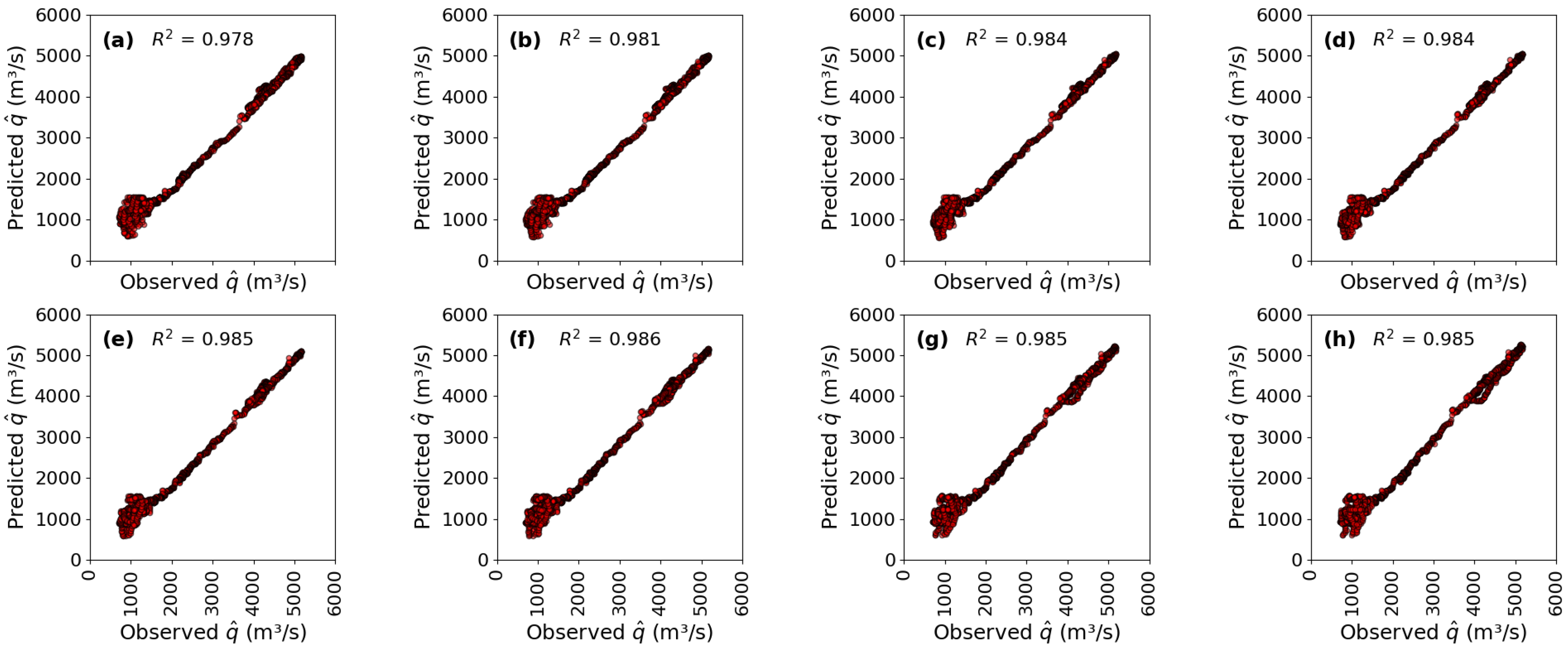
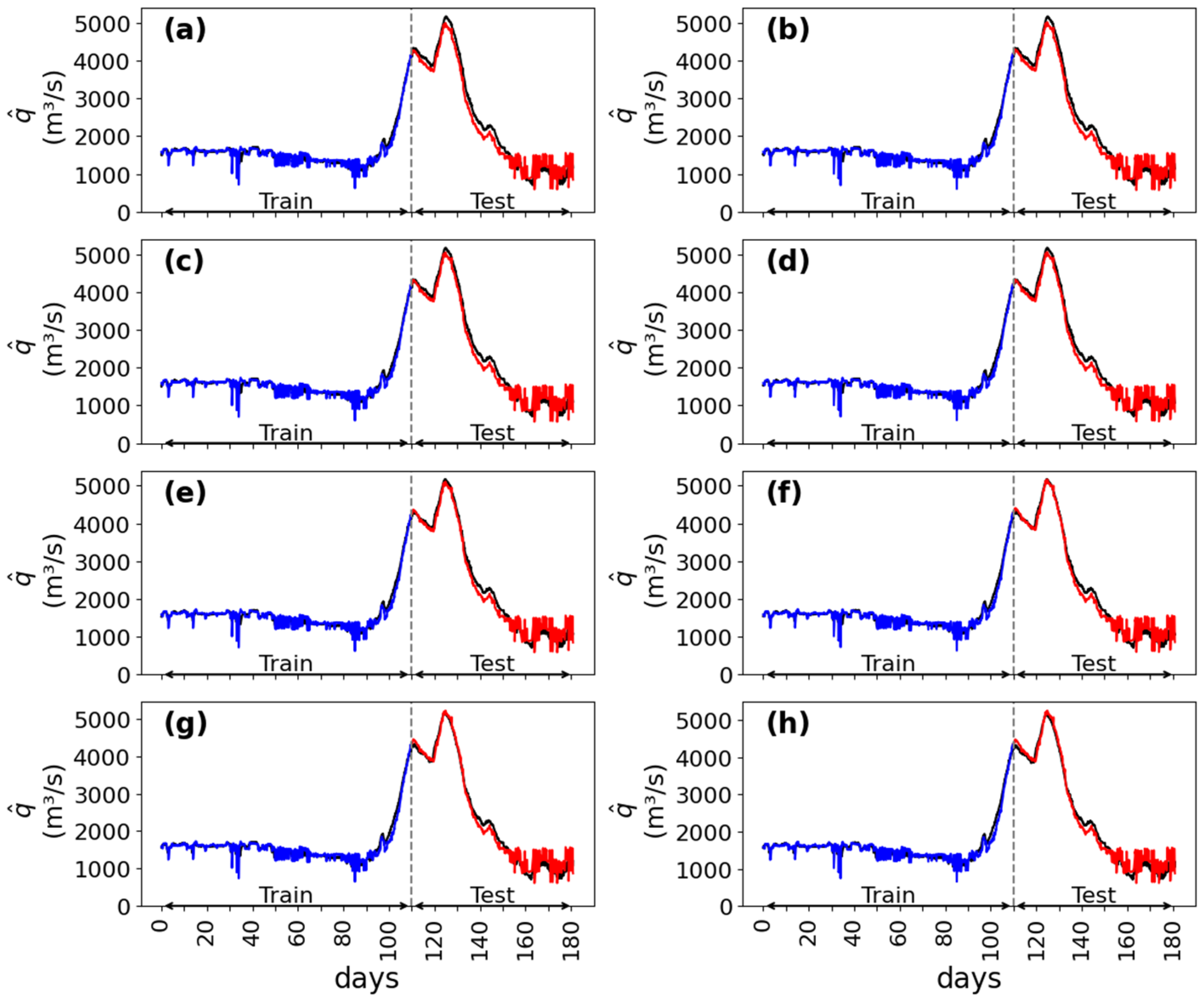
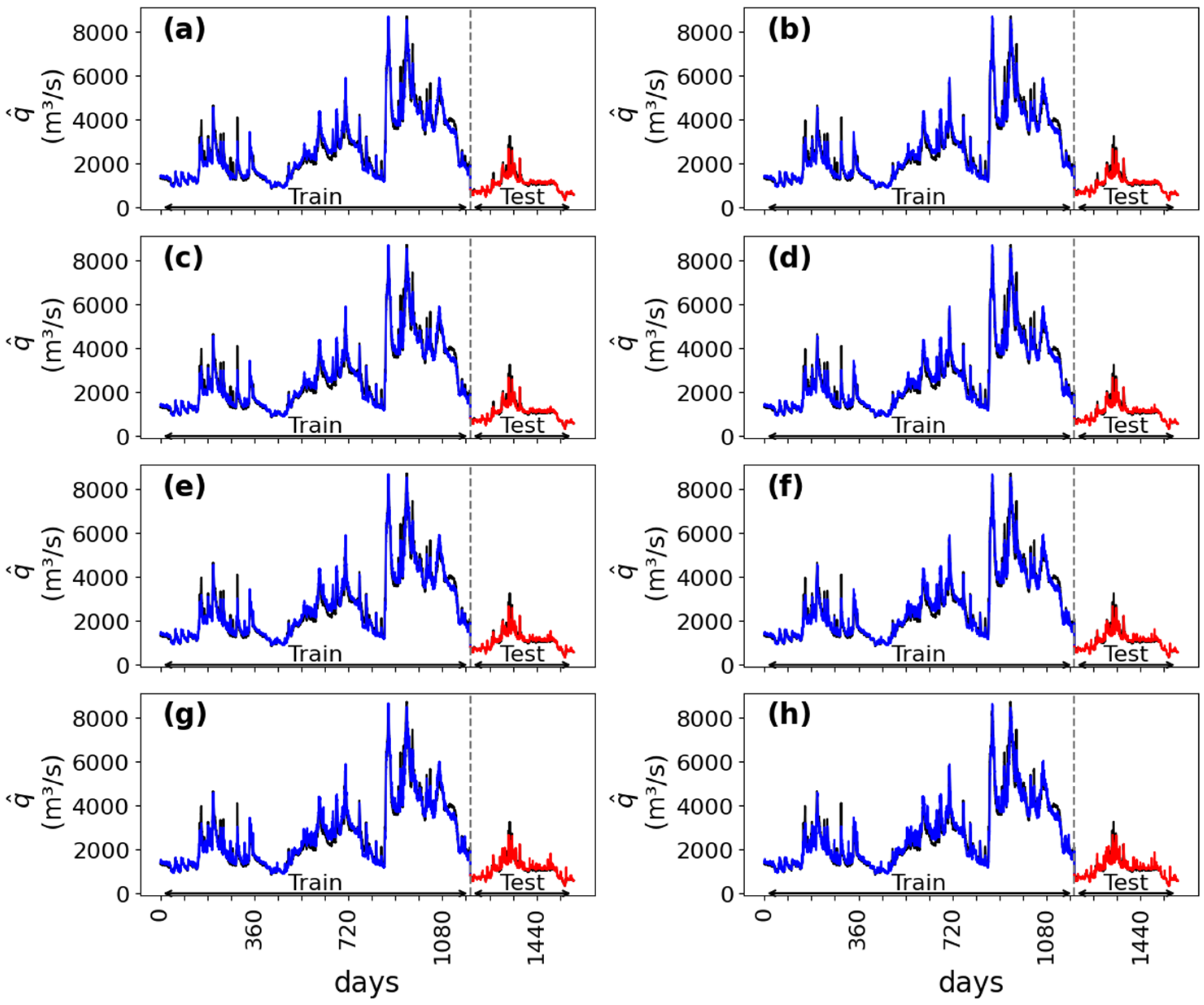
Using the test data points in Figure 5c,d and Figure 6e as input, the best model (Equation (14)) was used to predict discharge forecast q ^ at CSD (Figure 1) for eight given leading times. In Figure 7, the values of q ^ predicted using Equation (14) are compared with the corresponding test data points shown in Figure 7a. All comparisons show very strong correlations, with the coefficient of correlation ranging from 0.975 to 0.986. The results of the discharge forecast are particularly valuable for cases where the operations of CSD (Figure 1) have ceased and only historical data of q D exist. The results of q ^ effectively provide a spatiotemporal extension of the time series of discontinued data for a river CS, as illustrated in Figure 8.

3.5. Validation of the Best Model Equations

3.5.1. Discontinued Observation of Discharge at CSD

The best model equations (e.g., Equation (14) for δ t = 2 h) were validated through a reliability analysis using four statistical indicators (Equations (3)–(6)). Over the range of lead times δ t = 1–24 h, the TW for acceptable predictions (with F B 1 0 and F B 2 0 ) was determined. All leading times δ t = 1–24 h had F B 2 0 and δ t = 1–18 h had F B 1 0 . Short-term forecasts q ^ for δ t = 2, 4, 6, 8, 10, and 12 h were chosen for further data comparison. Data comparison was also made for larger lead times ( δ t = 16 and 18 h).
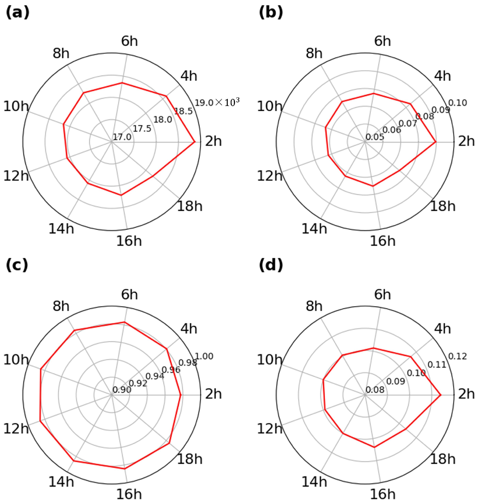
The statistical indicators of the analysis are shown in Figure 9. The values of AIC (Equation (6)) exhibited a decreasing trend, from c = 18,865 for δ t = 2 h to 18,070 for δ t = 12 h (Figure 9a), meaning that in a relative sense, the model equation (shown in Equation (14)) for δ t = 2 h was less reliable than that for δ t = 12 h. The normalised RMSE (Equation (4)) decreased from ε ~ = 8.4% for δ t = 2 h to 6.9% for δ t = 10 h, and then slightly increased to 7.5% at δ t = 18 h (Figure 9b). The coefficient of determination (Equation (3)) had large values, ranging from R 2 = 0.986 for δ t = 12 h to 0.978 for δ t = 2 h (Figure 9c). The mean absolute relative error (Equation (5)) gradually decreased from ε a = 12.0% for δ t = 2 h to 9.9% at δ t = 12 h (Figure 9d), indicating improved accuracy. ε a showed a minimum of 9.9% for δ t = 9 h.
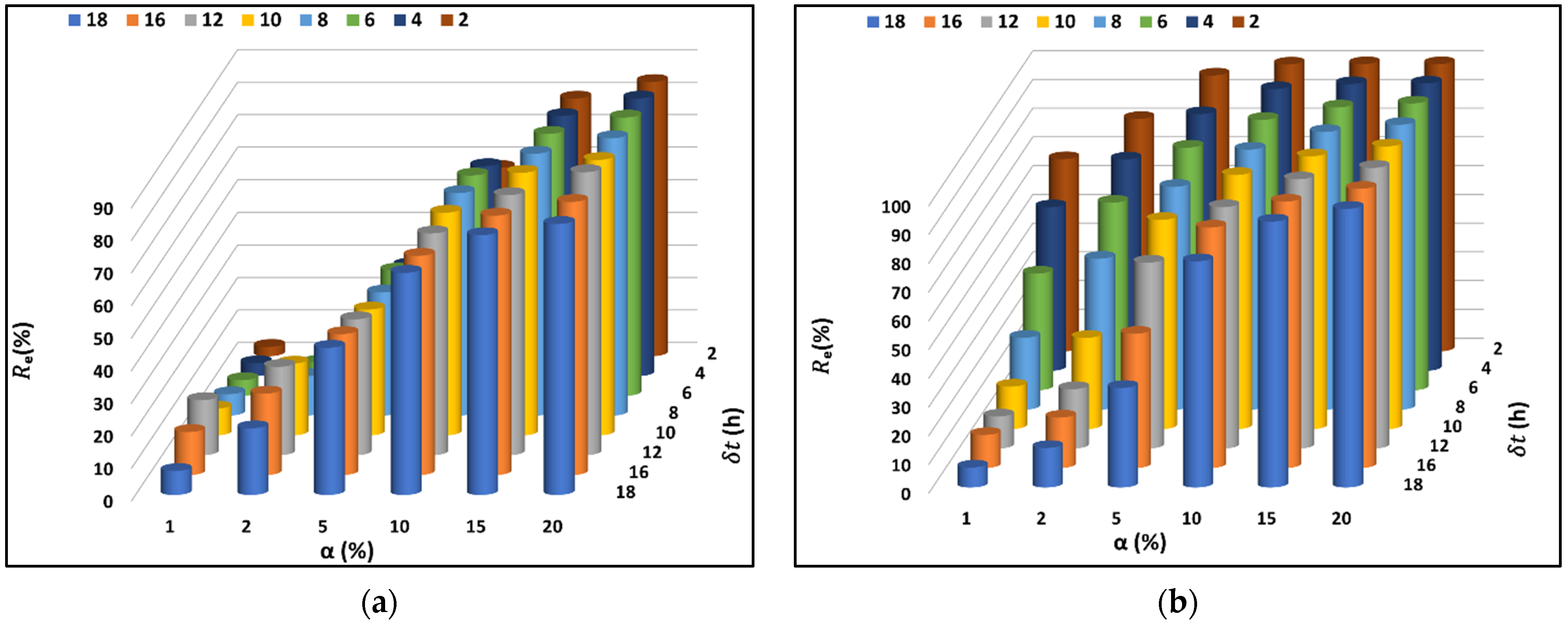
Values of the reliability R e (Equation (7)) for various leading times δ t and allowable relative errors α values are plotted in Figure 10a, where R e increased with increasing α. This is to say that reliability is lower if the allowable error is smaller. For example, if α was set to 1%, only 21% of the predicted discharges for δ t = 12 h had errors α < 1%. The percentage of the forecast discharges containing errors below 1% dropped to 17% for δ t = 12 h and to 3% for δ t = 2 h. As expected, it was difficult to obtain a reliable forecast for all leading times when the allowable error is very small (like α = 1%).
For larger α (say 5% or 10%), the reliability showed respective peak percentages of R e = 43% and 68% for δ t = 12 h, and the percentages dropped to 31% and 58% for δ t = 2 h (Figure 10a). A plausible explanation for the peak reliability is an advection time (time lag) of 12 h from the CSU to CSD. The uncertainties in discharge forecasts were higher for larger δ t . For α = 15%, approximately 80% of the predicted discharges contained errors below the error threshold.

3.5.2. Continuous Observation of Discharge at CSD

The best model equations (from input variables of q D , q U and T ) for the case of continuous discharge observation were validated using the same indicators as those used for the case of discontinued observation. Leading times δ t = 2, 4, 6, 8, 10, 12, 16, and 18 h were used for prediction. The values of c ranged from 10,977 for leading time δ t = 2 h, gradually decreasing to 18,175 for δ t = 18 h, meaning that the discharge forecast accuracy decreases with increasing leading time. The coefficient of determination was very close to unity for all leading times less than 12 h. The normalised RMSE was acceptable, ranging from 0.9% for δ t = 2 h to 7.4% for δ t = 18 h. The mean absolute relative error was also acceptable, in the range of 0.8–7.2%. The results given above indicate that the discharge forecast for 2 h leading time was more reliable than for other leading times.
One striking feature of the reliability distribution (Figure 10b) was that for a leading time δ t = 2 h, the values of reliability, R e , were high even when the allowable errors were very small, e.g., α = 2%. For all leading times, R e dropped as δ t increased. The reason is that the impact of the model input parameters on the output variable decreases with increasing leading time. For instance, for δ t = 2 h, R e = 0.75 when α was set to 1%, and 96.1% of the forecast discharges had a relative error below 5%, when compared to the corresponding observed values. The reliability was the lowest for δ t = 18 h for the given values of α , but there was still 92.5% of the forecast discharges with an error α 10%, and 97.0% with an error below 20%.

4. Discussion

The 1st degree polynomial models (e.g., Equations (11) and (14)) have shown a good reliability. This is supported by the principle of conservation of mass
q D = B   δ x δ t δ η + q U
where B is the channel width and δ η is the change of water level. The time-dependent flow from the CSU to CSD (Figure 3) is governed by this fundamental physical law, where q D , δ η , and q U are interrelated linearly. Such linearity corresponds to the 1st degree polynomial. Arguably, the automatic selection of the 1st degree polynomials in MGMDH has implicitly been informed by the physical law (Equation (17)).
At the same time, the flow is governed by the principle of the conservation of momentum
1 g δ q A δ t + q A g δ q A δ x + δ η δ x = S 0 S f
where g is the gravitational acceleration, A is cross-sectional area, q is the discharge, S f is the friction slope, and S 0 is the riverbed slope. The 2nd term on the left-hand side of Equation (18) introduces non-linearity to discharge relationship. For this reason, the 2nd or higher degree polynomial models, as MGMDH outputs, also have a physical basis, depending on the relative magnitude of the non-linear term. This can be one of the reasons that the 1st degree polynomial models introduce some errors in the discharge forecast. Note that compared to solving the time-dependent conservation equations, MGMDH offers a much more efficient and reasonably accurate discharge forecast, with high efficiency being crucial for real-time forecasting and management of river floods.
Although the reported polynomial models (Equations (11)–(16)) contain coefficients having site-specific values for the Ottawa River, the MGMDH is applicable to other similar river sites. This is demonstrated by applying the MGMDH to two CSs (USGS station ID: 13211205, and 13213000) of the Boise River in Idaho, U.S.A. They are located at 43°40′38″ N, 116°42′4″ W and 43°46′54″ N, 116°58′22″ W, respectively, and are about 30 km apart. The same procedures (Figure 4) were applied to time series of q U , η U , and T observed at 15-min intervals for the period of January 1–July 10, 2023. The results (Figure 11) demonstrate excellent performance, with R 2 = 0.910–0.996 (Equation (3)), ε ~ = 4.1–16.4% (Equation (4)), and R e = 90% when α is set to 10%.
Compared to other GMDH models (e.g., Ivakhnenko (1971) [40]; Letessier et al. (2023) [30]), the MGMDH in this paper included both linear and higher degree polynomials. This inclusion is useful for capturing complex patterns of river discharge data (Figure 8 and Figure 11), with minimal errors. This is a novel aspect of the current study. Some previous studies have overlooked the useful choice of linear polynomial models. The MGMDH can handle data gaps more effectively compared to GMDH and ASGMDH. The MGMDH is transparent, offering an explicit model equation (e.g., Equations (11)–(16)) for river engineers to use, as supposed to a black-box model.
In Figure 12, the performance of the MGMDH (applied to Ottawa River data for best and worst leading times δ t = 12 h (Figure 12a) and δ t = 2 h (Figure 12b), respectively) is compared to other two MLMs: adaptive structure of the group method of data handling (ASGMDH) and neural network (NN) that had five hidden layers and eight neurons. Figure 12 covered the complete list of statistical indicators given in Equations (3)–(6). The MGMDH slightly outperforms ASGMDH and NN in terms of c and R 2 and more significantly in terms of ε ~ and ε a . For more details about these four indicators for the ASGMDH, refer to Letessier et al. (2023) [30]. This can reflect that MGMDH has the capability to handle data with a wide variety of patterns, whereas ASGMDH can handle a limited variety of patterns. A plausible reason that MGMDH outperforms NN is NN’s tendency to overfit, especially with small or noisy datasets, and its complex structure that requires extensive tuning and may not always effectively capture underlying data patterns.
Take as an example a single data entry of discharge on 11 May 2023, at 6:00:00 AM. For δ t = 2 h, the observed discharge was 4310 m3/s, while the predicted discharge using Equation (14) was 4080 m3/s, resulting in a relative error ε a of 5%. In contrast, for δ t = 12 h, the observed discharge was 4240 m3/s, and the predicted discharge was 4206 m3/s (forecast equation is not listed), yielding a significantly lower relative error of 0.8%. This example shows improved forecast accuracy when the lead time is closer to the advection time. This alignment with the physical process likely improves the model’s R2 value, as the model’s predictive accuracy is more consistent when the forecast interval corresponds to the actual travel time of water between cross-sections. Therefore, choosing time intervals that reflect the natural advection time can significantly influence the overall performance and reliability of the model.
The model, intended primarily for real-time sub-diurnal discharge forecasting, can also be applied to daily forecasts. It has been used to forecast discharge at a 2-day lead time for the Ottawa and Boise rivers, showing a high accuracy with R 2 = 95% and ε ~ = 0.13 for the Ottawa River, and R 2 = 88% and ε ~ = 0.19 for the Boise River. Although the forecasts remain reliable for daily discharge, the accuracy decreases compared to sub-diurnal forecasting as lead time increases, as noted by Cheng et al. (2020) [26] and Nguyen et al. (2022) [46].
The MGMDH model has been primarily tested for floods in the Ottawa and Boise rivers during the ice melting period. However, it is suitable for predicting discharge over longer time periods. For example, for the Missouri River, the use of discharge data over the period of November 2016 to January 2020 from two stations (CSU ID: 06821250 and CSD ID: 06893000) gave predictions for the entire year of 2022 (Figure 13). The model exhibited high predictability performance, with R 2 = 0.9 at δ t = 2 , 4 , 6 , and 8 h, and R 2 0.854 at δ t = 24 h. The model is robust for long-term scenarios, which may be a discontinued case.
For continuous stations, changes in homogenisation due to topographic, hydraulic, or climatic conditions may initially impact the model reliability. However, as the model is continuously updated with new inputs, its accuracy improves over time. This adaptive approach aligns with ongoing management practices, refining predictions as new data becomes available.
For ceased stations, while minor impacts from climatic variations are anticipated, assuming regional similarities, it is crucial to consider these differences for model validity. The high variability of water-cycle processes, such as streamflow and precipitation, can be assessed through long-term persistence, often measured by the Hurst parameter [47]. Global analysis indicates that these processes typically exhibit a relatively high Hurst parameter [48], affecting their long-term predictability and thereby influencing expected reductions in lead time and time window.
The topography of river basins plays a significant role in altering flow regimes due to variations in elevation, slope, and land use between CSU and CSD. These differences can affect hydrological responses and necessitate careful consideration to maintain predictive accuracy. The sites in this study are situated along rivers that feature hydraulic structures, such as dams, which have the capacity to regulate flow patterns across extensive regions [49]. Hence, meticulous attention to these hydraulic influences is essential to mitigate errors and ensure reliable forecasts for ceased hydrometric stations.
A traditional rating curve may be established for a river CS and permits the conversion of observed water levels η D at the CS to discharges q D . The rating curve approach may not be feasible in certain situations, such as when a hydrometric station is ceased and η D data become unavailable. MGMDH can still be used if discharge and/or water level data are obtainable from a neighbouring station (e.g., Equations (11)–(13)). The operations of some existing hydrometrical stations may be suspended due to factors such as high costs, leaving data gaps for discharge. Such gaps can be filled using the cost-effective methods from this study. In addition, the methods can be used to address the influence of climate change on river discharge by adding air temperature and precipitation to predictors.
Nevertheless, the MGMDH should have limits on the minimum and the maximum number of predictors in order to enhance the reliability while mitigating potential accuracy issues. Including multiple predictors of discharge and water level aligns with the principles of the conservation of mass and of energy, which govern river flow. The use of a sole predictor is susceptible to a low reliability, possibly arising from errors in the measurements of the sole predictor. This vulnerability can be mitigated by including multiple predictors, which can help reduce the impact of missing or erroneous measurements of a particular predictor. Setting a limit on the maximum number of predictors helps prevent overfitting and saves computation time. It is important to strike a balance between reliability and efficiency in discharge forecast.
The model accuracy is significantly limited when relying solely on meteorological data without an active hydrometric station within the same river. Even if observations from a neighbouring station are used, these stations must be part of a homogeneous system with consistent climatic, topographic, and hydraulic conditions. However, the stations need not be in the same river reach, which adds complexity. Without hydrometric data from the river in question, the model’s reliability becomes questionable, potentially leading to inaccurate predictions.
One other limitation is that the ranking of predictors can possibly be unrealistic. For example, the dew point temperature was ranked higher than precipitation (Table 1). A plausible explanation is that the data analytics focused on correlations between predictors and the target variable rather than the underlying physical processes. Future studies should explore physics-informed ranking of predictors.
Errors can possibly arise in the selection of parameters, when the model calibration process achieves only a local minimum rather than the global minimum. This could result in suboptimal parameter values that do not accurately represent the system behaviour. Additionally, uncertainties in field observations, such as errors in the measurements of discharge or water level, can further propagate through the model, exacerbating prediction inaccuracies. In the absence of direct hydrometric data, such errors and uncertainties are expected to become more pronounced, significantly affecting the overall model performance. Accordingly, future research should focus on improving parameter calibration techniques to avoid local minima and refining methods to quantify and reduce observational uncertainties.

5. Conclusions

This paper reports an artificial intelligence model for the forecast of river discharge at continuous and ceased hydrometric stations. The model is a modified version of the group method of data handling (MGMDH). It is applied to two hydrometric stations of the Ottawa River in Ontario. The following conclusions have been reached:
  • The MGMDH automatically determines the best forecast model. The 1st degree model is consistent with the principle of mass conservation (Equation (17)). Higher degree models reflect the conservation of momentum. The models are efficient and accurate.
  • The MGMDH predicts a reliable forecast of river discharge at both active and ceased hydrometric CSs. The coefficient of determination, R 2 , is greater than 0.978 (Figure 7).
  • Forecasting of discharge at a ceased CS for a lead time close to the advection time from upstream to the CS is the most reliable.
  • The MGMDH developed for the Ottawa River is applicable to other rivers, as demonstrated in the successful application to the Boise River in Idaho, with R 2 > 0.9 (Figure 11).
  • The MGMDH outperforms other MLMs, like the black-box NN, for river discharge predictions (Figure 12). Compared to traditional rating curves, the MGMDH allows for forecasting and can include other predictors, such as meteorological parameters.
  • The automated selection of predictors is essential for river discharge forecasting. This improves model accuracy while minimising computing time, as discussed in Section 3.3.
This paper has contributed to the development of a simple, reliable framework for efficient forecasting of river discharge. This framework can serve as a tool to support river flood management and to generate hydrometric data as input to river engineering projects. The 1st degree polynomial models can introduce some errors in the forecast of discharge when patterns are complicated. It is recommended to limit the number of predictors to prevent overfitting and save computing time without a significant loss of accuracy.

Author Contributions

Conceptualisation, M.A.A.; Data algorithm and analysis, M.A.A.; Supervision, S.S.L.; Writing—original the draft, M.A.A.; Writing—review and editing, S.S.L.; Funding acquisition, S.S.L. All authors have read and agreed to the published version of the manuscript.

Funding

This study received financial support from the Natural Sciences and Engineering Research Council of Canada through Discovery Grants held by S.S.L. (grant number 2020-06796).

Data Availability Statement

All relevant data are included in the paper.

Acknowledgments

M.A.A. received on-leave approval from Ain Shams University, Cairo, Egypt.

Conflicts of Interest

The authors declare no conflicts of interest.

References

  1. Lešcěšen, I.; Basarin, B.; Pavić, D.; Mudelsee, M.; Pekarova, P.; Mesaroš, M. Are extreme floods on the Danube River becoming more frequent? A case study of Bratislava station. J. Water Clim. Change 2024, 15, 1300–1312. [Google Scholar] [CrossRef]
  2. Paterson, D.L.; Wright, H.; Harris, P.N.A. Health Risks of Flood Disasters. Clin. Infect. Dis. 2018, 67, 1450–1454. [Google Scholar] [CrossRef] [PubMed]
  3. Gaur, A.; Gaur, A.; Simonovic, S.P. Future Changes in Flood Hazards across Canada under a Changing Climate. Water 2018, 10, 1441. [Google Scholar] [CrossRef]
  4. Blöschl, G.; Hall, J.; Viglione, A.; Perdigão, R.A.P.; Parajka, J.; Merz, B.; Lun, D.; Arheimer, B.; Aronica, G.T.; Bilibashi, A.; et al. Changing climate both increases and decreases European river floods. Nature 2019, 573, 108–111. [Google Scholar] [CrossRef] [PubMed]
  5. Blöschl, G.; Hall, J.; Parajka, J.; Perdigão, R.A.P.; Merz, B.; Arheimer, B.; Aronica, G.T.; Bilibashi, A.; Bonacci, O.; Borga, M.; et al. Changing climate shifts timing of European floods. Science 2017, 357, 588–590. [Google Scholar] [CrossRef] [PubMed]
  6. Berghuijs, W.; Aalbers, E.; Larsen, J.; Trancoso, R.; Woods, R. Recent changes in extreme floods across multiple continents. Environ. Res. Lett. 2017, 12, 114035. [Google Scholar] [CrossRef]
  7. Alabbad, Y.; Yildirim, E.; Demir, I. Flood mitigation data analytics and decision support framework: Iowa Middle Cedar Watershed case study. Sci. Total Environ. 2022, 814, 152768. [Google Scholar] [CrossRef]
  8. Lins, H.F.; Slack, J.R. Seasonal and regional characteristics of U.S. streamflow trends in the United States from 1940 to 1999. Phys. Geogr. 2005, 26, 489–501. [Google Scholar] [CrossRef]
  9. Hirabayashi, Y.; Alifu, H.; Yamazaki, D.; Imada, Y.; Shiogama, H.; Kimura, Y. Anthropogenic climate change has changed frequency of past flood during 2010–2013. Prog. Earth Planet Sci. 2021, 8, 36. [Google Scholar] [CrossRef]
  10. Tabari, H. Climate change impact on flood and extreme precipitation increases with water availability. Sci. Rep. 2020, 10, 13768. [Google Scholar] [CrossRef]
  11. Li, M.; Wang, Q.J.; Robertson, D.E.; Bennett, J.C. Improved error modelling for streamflow forecasting at hourly time steps by splitting hydrographs into rising and falling limbs. J. Hydrol. 2017, 555, 586–599. [Google Scholar] [CrossRef]
  12. Agarwal, S.; Roy, P.; Choudhury, P.; Debbarma, N. Comparative study on stream flow prediction using the GMNN and wavelet-based GMNN. J. Water Clim. Chang. 2022, 13, 3323–3337. [Google Scholar] [CrossRef]
  13. Khosravi, K.; Cooper, J.R.; Daggupati, P.; Thai Pham, B.; Tien Bui, D. Bedload transport rate prediction: Application of novel hybrid data mining techniques. J. Hydrol. 2020, 585, 124774. [Google Scholar] [CrossRef]
  14. Ekwueme, B.N. Deep neural network modeling of river discharge in a tropical humid watershed. Earth Sci. Inform. 2024, 17, 1161–1177. [Google Scholar] [CrossRef]
  15. Liu, Y.; Wang, H.; Feng, W.; Huang, H. Short term real-time rolling forecast of urban river water levels based on LSTM: A case study in Fuzhou city, China. Int. J. Environ. Res. Public Health 2021, 18, 9287. [Google Scholar] [CrossRef] [PubMed]
  16. Garg, N.; Negi, S.; Nagar, R.; Rao, S.; Seeja, K.R. Multivariate multi-step LSTM model for flood runoff prediction: A case study on the Godavari River Basin in India. J. Water Clim. Chang. 2023, 14, 3635–3647. [Google Scholar] [CrossRef]
  17. Haznedar, B.; Kilinc, H.C.; Ozkan, F.; Yurtsever, A. Streamflow forecasting using a hybrid LSTM-PSO approach: The case of Seyhan Basin. Nat. Hazards 2023, 117, 681–701. [Google Scholar] [CrossRef]
  18. Li, J.; Yuan, X.; Ji, P. Long-lead daily streamflow forecasting using Long Short-Term Memory model with different predictors. J. Hydrol. Reg. Stud. 2023, 48, 101471. [Google Scholar] [CrossRef]
  19. Tan, W.Y.; Lai, S.H.; Pavitra, K.; Teo, F.Y.; El-Shafie, A. Deep learning model on rates of change for multi-step ahead streamflow forecasting. J. Hydroinform. 2023, 25, 1667–1689. [Google Scholar] [CrossRef]
  20. Kao, I.F.; Zhou, Y.; Chang, L.C.; Chang, F.J. Exploring a Long Short-Term Memory based Encoder-Decoder framework for multi-step-ahead flood forecasting. J. Hydrol. 2020, 583, 124631. [Google Scholar] [CrossRef]
  21. Jhong, Y.-D.; Lin, H.P.; Chen, C.S.; Jhong, B.C. Real-time Neural-network-based Ensemble Typhoon Flood Forecasting Model with Self-organizing Map Cluster Analysis: A Case Study on the Wu River Basin in Taiwan. Water Resour. Manag. 2022, 36, 3221–3245. [Google Scholar] [CrossRef]
  22. Skoulikaris, C.; Nagkoulis, N. A genetic algorithm’s novel rainfall distribution method for optimized hydrological modeling at basin scales. J. Hydroinform. 2024, 26, 1295–1312. [Google Scholar] [CrossRef]
  23. Girihagama, L.; Naveed Khaliq, M.; Lamontagne, P.; Perdikaris, J.; Roy, R.; Sushama, L.; Elshorbagy, A. Streamflow modelling and forecasting for Canadian watersheds using LSTM networks with attention mechanism. Neural Comput. Appl. 2022, 34, 19995–20015. [Google Scholar] [CrossRef]
  24. Alizadeh, B.; Ghaderi Bafti, A.; Kamangir, H.; Zhang, Y.; Wright, D.B.; Franz, K.J. A novel attention-based LSTM cell post-processor coupled with bayesian optimization for streamflow prediction. J. Hydrol. 2021, 601, 126526. [Google Scholar] [CrossRef]
  25. Adnan, R.M.; Liang, Z.; Trajkovic, S.; Zounemat-Kermani, M.; Li, B.; Kisi, O. Daily streamflow prediction using optimally pruned extreme learning machine. J. Hydrol. 2019, 577, 123981. [Google Scholar] [CrossRef]
  26. Cheng, M.; Fang, F.; Kinouchi, T.; Navon, I.M.; Pain, C.C. Long lead-time daily and monthly streamflow forecasting using machine learning methods. J. Hydrol. 2020, 590, 125376. [Google Scholar] [CrossRef]
  27. Kheimi, M. Data-driven approaches for estimation of sediment discharge in rivers. Earth Sci. Inform. 2023, 17, 761–781. [Google Scholar] [CrossRef]
  28. MacKenzie, K.M.; Gharabaghi, B.; Binns, A.D.; Whiteley, H.R. Early detection model for the urban stream syndrome using specific stream power and regime theory. J. Hydrol. 2022, 604, 127167. [Google Scholar] [CrossRef]
  29. Mohanta, A.; Pradhan, A.; Mallick, M.; Patra, K.C. Assessment of Shear Stress Distribution in Meandering Compound Channels with Differential Roughness Through Various Artificial Intelligence Approach. Water Resour. Manag. 2021, 35, 4535–4559. [Google Scholar] [CrossRef]
  30. Letessier, C.; Cardi, J.; Dussel, A.; Ebtehaj, I.; Bonakdari, H. Enhancing Flood Prediction Accuracy through Integration of Meteorological Parameters in River Flow Observations: A Case Study Ottawa River. Hydrology 2023, 10, 164. [Google Scholar] [CrossRef]
  31. Yarahmadi, M.B.; Parsaie, A.; Shafai-Bejestan, M.; Heydari, M.; Badzanchin, M. Estimation of Manning Roughness Coefficient in Alluvial Rivers with Bed Forms Using Soft Computing Models. Water Resour. Manag. 2023, 37, 3563–3584. [Google Scholar] [CrossRef]
  32. Souza, D.P.M.; Martinho, A.D.; Rocha, C.C.; Christo, E.d.S.; Goliatt, L. Hybrid particle swarm optimization and group method of data handling for short-term prediction of natural daily streamflows. Model. Earth Syst. Environ. 2022, 8, 5743–5759. [Google Scholar] [CrossRef]
  33. Elkurdy, M.; Binns, A.D.; Bonakdari, H.; Gharabaghi, B.; McBean, E. Early detection of riverine flooding events using the group method of data handling for the Bow River, Alberta, Canada. Int. J. River Basin Manag. 2022, 20, 533–544. [Google Scholar] [CrossRef]
  34. Bruno, L.S.; Mattos, T.S.; Oliveira, P.T.S.; Almagro, A.; Rodrigues, D.B.B. Hydrological and Hydraulic Modeling Applied to Flash Flood Events in a Small Urban Stream. Hydrology 2022, 9, 223. [Google Scholar] [CrossRef]
  35. Erima, G.; Kabenge, I.; Gidudu, A.; Bamutaze, Y.; Egeru, A. Differentiated Spatial-Temporal Flood Vulnerability and Risk Assessment in Lowland Plains in Eastern Uganda. Hydrology 2022, 9, 201. [Google Scholar] [CrossRef]
  36. Mentzafou, A.; Dimitriou, E. Hydrological Modeling for Flood Adaptation under Climate Change: The Case of the Ancient Messene Archaeological Site in Greece. Hydrology 2022, 9, 19. [Google Scholar] [CrossRef]
  37. Filianoti, P.; Gurnari, L.; Zema, D.A.; Bombino, G.; Sinagra, M.; Tucciarelli, T. An evaluation matrix to compare computer hydrological models for flood predictions. Hydrology 2020, 7, 42. [Google Scholar] [CrossRef]
  38. Yang, X.; Liu, Q.; He, Y.; Luo, X.; Zhang, X. Comparison of daily and sub-daily SWAT models for daily streamflow simulation in the Upper Huai River Basin of China. Stoch. Environ. Res. Risk Assess. 2016, 30, 959–972. [Google Scholar] [CrossRef]
  39. Sun, Y.; Zhang, L.; Liu, J.; Lin, J.; Cui, Q. A Data Assimilation Approach to the Modeling of 3D Hydrodynamic Flow Velocity in River Reaches. Water 2022, 14, 3598. [Google Scholar] [CrossRef]
  40. Ivakhnenko, A.G. Polynomial Theory of Complex Systems. IEEE Trans. Syst. Man. Cybern. 1971, 1, 364–378. [Google Scholar] [CrossRef]
  41. Montgomery, D.C.; Runger, G.C. Applied Statistics and Probability for Engineers. Eur. J. Eng. Educ. 1994, 19, 383. [Google Scholar] [CrossRef]
  42. Hipni, A.; El-shafie, A.; Najah, A.; Karim, O.A.; Hussain, A.; Mukhlisin, M. Daily Forecasting of Dam Water Levels: Comparing a Support Vector Machine (SVM) Model With Adaptive Neuro Fuzzy Inference System (ANFIS). Water Resour. Manag. 2013, 27, 3803–3823. [Google Scholar] [CrossRef]
  43. Modaresi, F.; Araghinejad, S. A comparative assessment of support vector machines, probabilistic neural networks, and K-nearest neighbor algorithms for water quality classification. Water Resour. Manag. 2014, 28, 4095–4111. [Google Scholar] [CrossRef]
  44. Ebtehaj, I.; Bonakdari, H. A reliable hybrid outlier robust non-tuned rapid machine learning model for multi-step ahead flood forecasting in Quebec, Canada. J. Hydrol. 2022, 614, 128592. [Google Scholar] [CrossRef]
  45. Dimitriadis, P.; Koutsoyiannis, D.; Tzouka, K. Predictability in dice motion: How does it differ from hydro-meteorological processes? Hydrol. Sci. J. 2016, 61, 1611–1622. [Google Scholar] [CrossRef]
  46. Nguyen, D.H.; Le, X.H.; Anh, D.T.; Kim, S.H.; Bae, D.H. Hourly streamflow forecasting using a Bayesian additive regression tree model hybridized with a genetic algorithm. J. Hydrol. 2022, 606, 127445. [Google Scholar] [CrossRef]
  47. Hurst, H.E. Long-Term Storage Capacity of Reservoirs. Trans. Am. Soc. Civ. Eng. 1951, 116, 770–808. [Google Scholar] [CrossRef]
  48. Dimitriadis, P.; Koutsoyiannis, D.; Iliopoulou, T.; Papanicolaou, P. A global-scale investigation of stochastic similarities in marginal distribution and dependence structure of key hydrological-cycle processes. Hydrology 2021, 8, 59. [Google Scholar] [CrossRef]
  49. Poff, N.L.R.; Olden, J.D.; Merritt, D.M.; Pepin, D.M. Homogenization of regional river dynamics by dams and global biodiversity implications. Proc. Natl. Acad. Sci. USA 2007, 104, 5732–5737. [Google Scholar] [CrossRef]
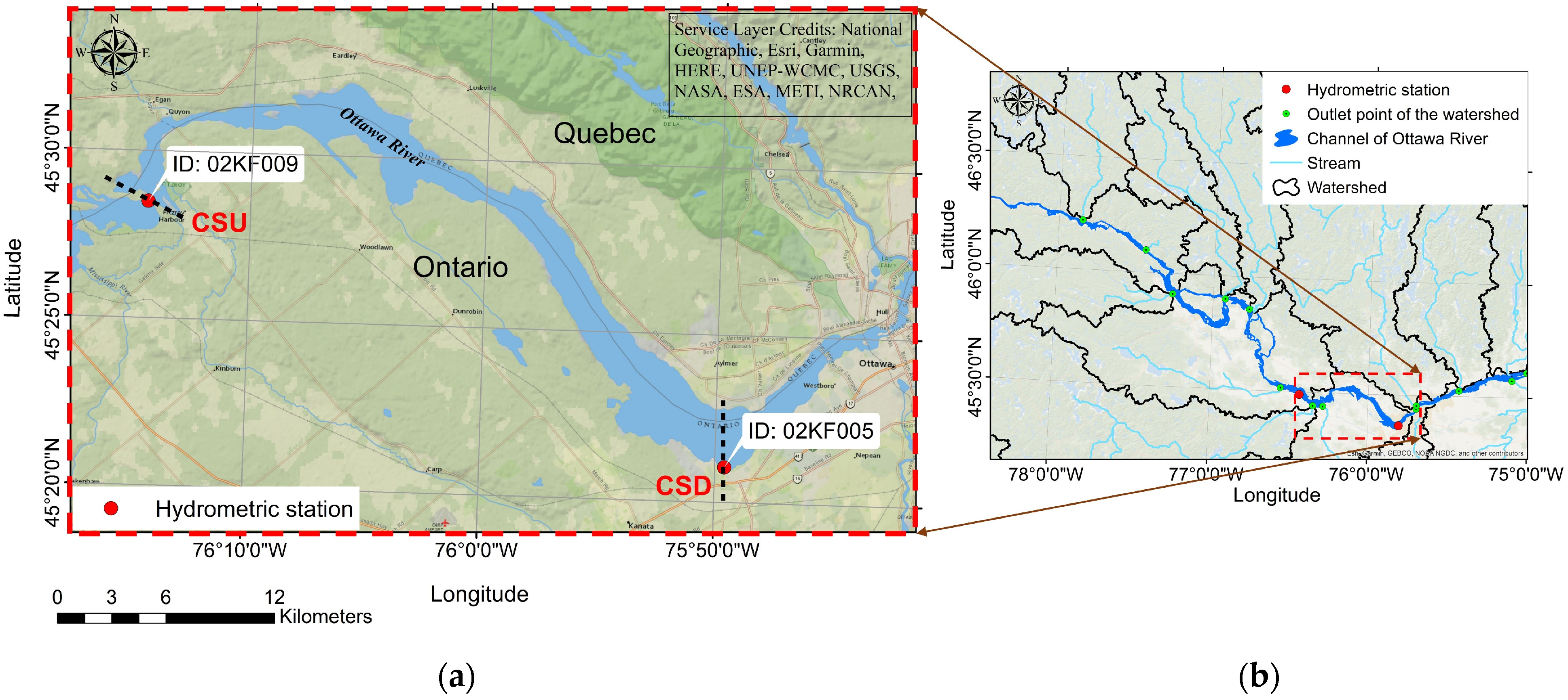
Figure 1. (a) Close-up view of the Ottawa River between hydrometric stations 02KF009 (CS upstream or CSU) and 02KF005 (CS downstream or CSD); (b) broad view of the stream network, watershed boundaries, and outlet points, illustrating how these watersheds flow into and connect with the Ottawa River.
Hydrology 11 00151 g001
Figure 2. Schematic time series of continuous observations of q (solid black curve), discontinued observations of q (solid red curve), and predicted future values of q ^ (dashed curves).
Hydrology 11 00151 g002
Figure 3. Definition diagram of river flow: (a) top view of the river channel; (b) CS at upstream (CSU) with discharge q U and water level η U (above a certain reference datum); (c) CS at downstream (CSD) with discharge q D and water level η D .
Hydrology 11 00151 g003
Figure 4. Flowchart of the methods for river discharge forecast.
Hydrology 11 00151 g004
Figure 5. Time series of hourly averaged variable: (a) discharge q D ; (b) water level η D , observed from the CS of interest (02KF005); (c) discharge q U ; (d) water level η U , observed from 02KF009, covering a period of 180 days (1 January–30 June 2023). The dotted lines divide the time series into two parts: one for model training, and the other for model testing (the same in subsequent figures).
Hydrology 11 00151 g005
Figure 6. Time series of observed hourly averaged variable: (a) T ; (b) θ ; (c) ϕ ; (d) P a t m ; (e) P for the period of 1 January–30 June 2023 at WMO station (ID: 71063) located at 45°23′00″ N, 75°43′00″ W.
Hydrology 11 00151 g006
Figure 7. Values of q ^ predicted from Equation (14) for lead times: (a) δ t = 2, (b) 4, (c) 6, (d) 8, (e) 10, (f) 12, (g) 16, and (h) 18 h, in comparison with observed q D (test data points in Figure 5a).
Hydrology 11 00151 g007
Figure 8. Time series of hourly-averaged discharges, observed at CSD (black curve), and forecasted using Equation (14) for the training period (blue curve) and for the testing period (red curve). The forecast is for lead times: (a) δ t = 2; (b) 4; (c) 6; (d) 8; (e) 10; (f) 12; (g) 16; and (h) 18 h.
Hydrology 11 00151 g008
Figure 9. Performance of the forecast model: (a) AIC c; (b) normalised RMSE ε ~ ; (c) the coefficient of determination R 2 ; (d) mean absolute relative error ε a .
Hydrology 11 00151 g009
Figure 10. Reliability (Equation (7)) of the best model functions for: (a) the case of discontinued discharge observation; and (b) the case of continuous discharge observation.
Hydrology 11 00151 g010
Figure 11. Time series of 15-min-averaged discharges, observed at CSD of the Boise River (black curve), and forecasted for the training period (blue curve) and for the testing period (red curve). The forecast is for lead times: (a) δ t = 2; (b) 4; (c) 6; (d) 8; (e) 10; (f) 12; (g) 18; and (h) 24 h.
Hydrology 11 00151 g011
Figure 12. Comparison of performance between MGMDH and other MLMs. The lead time is: (a) δ t = 12 h; and (b) δ t = 2 h.
Hydrology 11 00151 g012
Figure 13. Time series of hourly averaged discharges, observed at CSD of the Missouri River (black curve), and forecasted for the training period (blue curve) and for the testing period (red curve). The forecast is for lead times: (a) δ t = 2; (b) 4; (c) 6; (d) 8; (e) 10; (f) 12; (g) 18; and (h) 24 h.
Hydrology 11 00151 g013
Table 1. Predictors and values of ε for various degree polynomial functions. The ranking of the predictors as the best sole predictor is for lead time δ t = 2 h.
Predictor NMSE   ε Rank
1st Degree Polynomial2nd Degree Polynomial3rd Degree Polynomial
q D 0.002 a0.0031.1031
η D 0.0390.002 a0.5182
q U 0.134 a1.9574.0783
η U 0.500 a0.832888.3624
θ 1.2901.3521.176 a5
P 1.183 a1.1841.1916
P a t m 1.200 a1.2061.2267
ϕ 1.2841.2901.252 a8
T1.379 a1.5021.5999
a best among the 1st, 2nd and 3rd degree polynomial functions for the same sole predictor.
Disclaimer/Publisher’s Note: The statements, opinions and data contained in all publications are solely those of the individual author(s) and contributor(s) and not of MDPI and/or the editor(s). MDPI and/or the editor(s) disclaim responsibility for any injury to people or property resulting from any ideas, methods, instructions or products referred to in the content.