Article

Development of Statistical Downscaling Model Based on Volterra Series Realization, Principal Components, Climate Classification, and Ridge Regression

Department of Civil and Environmental Engineering, University of Auckland, Auckland 1010, New Zealand
*
Author to whom correspondence should be addressed.
Hydrology 2024, 11(9), 144; https://doi.org/10.3390/hydrology11090144
Submission received: 19 July 2024 / Revised: 21 August 2024 / Accepted: 27 August 2024 / Published: 10 September 2024

Abstract

:
This paper applied the fuzzy function approach, combined with the ridge regression model, to produce daily rainfall projections from large-scale climate variables. This study developed a statistical downscaling model based on principal components, c-means fuzzy clustering, Volterra series, and ridge regression. The model is known, hereafter as SDC2R2. In the developed downscaling model, the use of ridge regression, instead of multiple linear regression, is proposed to downscale daily rainfall with wide range (WR) predictors. The WR predictors were applied to sufficiently incorporate climate change signals. The developed model also captured the non-linear interactions of the climate variables by applying the transformation of Volterra series realization over WR predictors. This transformation was performed by applying principal components as orthogonal filters. Further, these principal components were clustered by using c-means clustering and non-linear transformations were applied on these membership functions, to improve the prediction ability of the model. The reanalysis of climate data from the National Centres for Environmental Prediction (NCEP) was used to develop the model and was validated by using the Global Climate Model (GCM) for four locations in the Manawatu River basin. The developed model was used to obtain future daily rainfall projections from three Representative Concentrative Pathways (RCP 2.6, RCP 4.5, and RCP 8.5) scenarios from the Canadian Earth System Model (CanESM2) GCM. The performance of the model was compared with a widely used statistical downscaling model (SDSM). It was observed that the model performed better than SDSM in downscaling rainfall on a daily basis. Every scenario indicated that there is a probability of obtaining high future rainfall frequency. The results of this study provide valuable information for decision-makers since climate change may potentially impact the Manawatu basin.

1. Introduction

The climate change influence over hydrological cycle is altering water resources considerably. The future projections of climate change are obtained by using different emission scenarios of Global Circulation Models (GCMs) [1]. The GCMs can simulate the large-scale atmospheric variables with optimum accuracy but these outputs cannot be directly used to assess the climate change impacts on local scale hydrological variables, such as rainfall. The potential cause for this failure is mainly due to the mismatch between the spatial resolutions of GCMs and that of hydrological models. In principle, the GCMs are three-dimensional models, which provide spatial coverage at the global scale (ranges from 250 to 600 km) while the hydrological models are at much finer scales (ranges up to a few hundred km). Furthermore, the goal of evaluating the climate impacts at the local scale is obtained using downscaling methods. Downscaling is the process of converting the coarser resolution data to finer resolution data, which can involve the generation of the hydrological variable at a specific area using the GCM outputs. The downscaling methods are mainly classified as dynamical and statistical downscaling techniques. It is widely reported that statistical downscaling techniques are simple to use and the area of interest can be easily transferred from one place to another, thus they are preferred over dynamical downscaling techniques [2]. Statistical downscaling is classified as, namely: (i) weather generator, (ii) weather typing, and (iii) multiple regression, which is specifically used to develop empirical relationships between the predictors (large-scale variables) and the predictand (small-scale variable). In particular, statistical downscaling is also preferred because it does not directly need the knowledge of the region’s physical processes to establish the statistical relationship between local variables, climate variables, and GCMs’ output [3]. Thus, statistical downscaling is broadly used by researchers to obtain projections based on the climate studies [3,4].
Despite the fact that the statistical downscaling models are very popular and extensively used in many studies, it is observed that they perform well only under those conditions and regions for which they were developed [5]. The credibility of the statistical downscaling technique is dependent on the stability of the predictor and predictand relationship. Basically, the statistical relationship is established by the subjective choice of predictors. In this context, the predictor selection and preparation are crucial for successful downscaling. Generally, the predictor selection is based on correlation analysis [6,7]. Hewitson and Crane (1996) mentioned that the chosen predictors could perform successful downscaling by fulfilling all three of the following criteria: (i) the chosen GCM reproduces large-scale predictors appropriately, (ii) the relationship between predictors and predictand is valid, even outside the calibration period, and (iii) the chosen predictor set is strongly incorporating climate change signals. Furthermore, the most important criterion is that the predictors and predictand relationship should also be valid even outside the calibration period, which is the most difficult target to fulfill by the restricted choice of predictors [8]. Therefore, Wetterhall (2005) suggested working with wide range predictors, which will cover all three aspects required for successful downscaling [8]. Singh et al. (2023) worked with wide range (WR) predictors to fulfil all criteria of the successful downscaling and improved performance of the statistical downscaling model [9]. However, a variety of techniques associated with certain strengths and weaknesses are available to establish the statistical downscaling model. Owing to the simple application and the low computational cost, several machine-learning and statistical approaches are applied in the field of climate downscaling. Some machine-learning approaches include relevance vector machines [10], support vector machines [6,11], the regression-based statistical downscaling model (SDSM) [12,13], and Gene Expression programming (GEP) [13]. Even though these machine-learning approaches are popular, due to their black-box nature they are often criticized. The underlying process between the predictors and predictand relationship is generally unknown. Govindaraju (2005) noted that the traditional ANN models suffer from the possibility of getting trapped in the local minima [11]. Similarly, the support vector machine performance is affected by the size of the training data set and the absence of probabilistic interpretation. Generally, natural processes are non-stationary and thus work at different temporal and spatial scales. Any models designed for climate downscaling will produce more realistic results if they are capable of capturing these spatial variabilities [12], therefore, it is essential to understand the spatial variability of the region.
Machiwal et al. (2019) mentioned that rainfall is highly variable over space and time, and it can be regarded as a good indicator of climate change and variability [13]. Consequently, several methods were used to investigate the spatial rainfall patterns, such as harmonic analysis [14], multivariate regression [15], spatial interpolation [16], k-means clustering [17], regional frequency analysis [18], and support vector machines [19]. Some research studies also applied Cluster Analysis (CA) and Principal Component Analysis (PCA) to specify the rainfall patterns. Amissah-Arthur and Jagtap (1999) identified decreasing rainfall trends in four delineated groups by the application of PCA and CA [20]. Ghosh and Mujumdar (2006) developed a downscaling model to study future droughts under climate change. The model was developed by clustering principal components into different clusters (c-means clustering) to regress the observed rainfall data with multiple linear regression (MRA) and obtained the future projections of monthly rainfall with 90% accuracy [21]. Machiwal et al. (2019) applied hierarchical cluster analysis (HCA) over 62 stations in the western arid region of India, to inspect the spatial patterns of monthly, seasonal, and annual rainfall, which are vital for planners and decision-makers to articulate a master plan to manage unexpected rainfall quantities [13].
The fuzzy function approach based on the regression model produces successful results for the prediction problems [22]. The fuzzy functions are obtained by applying some transformation over the input (explanatory) variables. Bas et al. (2019) mentioned that the transformation applied should be non-linear, as the linear relationship between explanatory variables in MRA leads to multi-collinearity [22]. Also, this multi-collinearity causes an increase in the variance of regression estimators, which leads to inconsistent results. The Principal Component Analysis (PCA) and the ridge regression (RR) are the potential solutions to be used in the presence of multi-collinearity. PCA is applied to address the multi-collinearity of the variables by extracting the important principal components (PCs) for model development. In addition, the principal components could be used as an orthogonal filter over the climate variables to obtain the realization of Volterra series expansion. Watanabe (1986) described that “the sum of powers of the outputs from the orthogonal filter is considered as the model, and the coefficient of the terms in the model are determined so that the mean square error between the outputs of the system to be measured and the model is minimized” [23]. Additionally, the Volterra model is applied to model climate inputs [24], as the Volterra model successfully addresses the non-linear behaviour of the geophysical state variables by producing a comprehensive representation of the non-linear natural systems [25].
In a previous study, Ghosh and Mujumdar (2006) projected monthly rainfall with 90% accuracy for the assessment of climate change’s impact on future droughts. The monthly rainfall projections were obtained by a downscaling model, which was developed by a combination of techniques, namely, multiple linear regression, principal component analysis (PCA), c-means clustering, and seasonality. A matter of fact is that the regression estimates generated by MLA are unstable due to multi-collinearity, and Hoerl and Kennard (1970) mentioned that another important remedy to model the multi-collinearity problem is ridge regression (RR) [26]. In comparison to the ordinary least square (OLS) method used in regression analysis, the RR has two major advantages: (i) it works on multi-collinearity, and (ii) it also decreases the mean square error (MSE) of the predictors. Hoerl et al. (1975) proposed a formula to obtain shrinkage parameters in RR. The shrinkage parameter, also known as the ridge parameter, has small positive values, which helps in dealing with multi-collinearity and minimizing the mean square error of the observed and predicted data [27]. Thus, the motivation of this paper is to apply an orthogonal filter obtained from PCA, which was used to generate the explanatory variables generated as a realization of Volterra series expansions to address the non-linear behaviour of the system. The application of c-means fuzzy clustering further strengthened the model’s ability to capture the non-linear interactions of the climate variables at both temporal and spatial scales, which means capturing the relationship variability of predictand and predictors at different time scales. Additionally, the non-linear transformation was applied to the membership functions as exponential and logarithmic transformation, which improves the model prediction ability. Finally, the SDC2R2 model is developed with Fuzzy RR instead of Fuzzy MLR to deal with the multi-collinearity of membership functions developed due to the transformations and deliver more accurate rainfall projections by producing stable coefficient estimates.

2. Study Area and Data Used

The study area has four rainfall gauging stations—Palmerston, Marton, Opiki and Te Rehunga, located in the Manawatu catchment, New Zealand, shown in Figure 1. The catchment has a warm and temperate climate zone. It also has high rainfall variability, which ranges from 900 mm to 1500 mm. The most significant natural hazard of the catchment is flooding, which is likely to become more intensified and frequent due to atmospheric changes caused by climate change [28]. Thus, the essential component of impact assessment is to obtain future rainfall projections at local scales. Therefore, to assist climate change impact at local scales, we choose the Manawatu catchment to implement the downscaling approach to generate future rainfall projections provided by the GCMs. This study used the daily observed rainfall data as the local scale predictand, obtained from the National Climate Database (http://cliflo.niwa.co.nz/) accessed in 1 January 2021. Similar to previous downscaling studies, the National Centers for Environmental Prediction (NECP) reanalysis data was used as the large-scale predictors for the development of the statistical downscaling model [29,30]. The large-scale reanalysis datasets were obtained from the NCEP/NCAR reanalysis gridded datasets CanESM2 project (Canadian site http://climate-scenarios.canada.ca/, accessed on 1 January 2021). This study used the CanESM2 dataset because this dataset is widely used in hydrological and climate change studies, because of its global coverage [31]. Chim et al. (2020) noted that numerous studies, such as Rashid et al. (2016) [32] and Agarwal et al. (2017) [33], have achieved successful downscaling results using the CanESM2 dataset [31]. CanESM2 is developed by Environment and Climate Change Canada (ECCC). The CanESM2 model has a spatiotemporal resolution of approximately 2.8 degrees latitude by 2.8 degrees longitude. This means that each grid cell of the model covers a region roughly 2.8 degrees by 2.8 degrees in geographic coordinates. Additionally, CanESM2 generally provides output at monthly or daily intervals, depending on the specific dataset or simulation being used.
Furthermore, the large-scale predictors of GCMs were also obtained from the same Canadian site (NCEP). The three different Representative Concentration Pathway (RCP) scenarios used for the future projections are: RCP 2.6 (low emission scenario that leads radiative forcing (RF) to 3.1 W/m2 by 2035 and drops to 2.6 W/m2 by 2100), RCP 4.5 (medium stabilization scenario that leads RF to 4.5 W/m2 beyond 2100), and RCP 8.5 (high emission scenario that leads RF to 8.5 W/m2 by 2100). Additionally, the identification of these pathways is based on greenhouse and aerosol concentrations, which will be produced by the end of the century. The climate downscaling in the Manawatu River basin was previously studied by Singh et al. (2023) [9], and the selected predictors were strong contributors to the variability of rainfall in the region. Thus, based on their documentation, a total of 20, 16, 19, and 21 predictors were considered for Palmerston, Marton, Opiki, and Te Rehunga stations, respectively.

3. Tools and Techniques

In this study, several methods are used for the development of the downscaling model, as well as for benchmarking the results of the developed downscaling model. These methods are the statistical downscaling model (SDSM), the Multiple Linear Regression (MLR), the Principal Component Analysis (PCA), the Volterra Series Expansion, the c-means clustering, and the ridge regression. The first two methods are regression-based downscaling models, which primarily depend on developing a predictor and predictand relationship. Although these are popular traditional single-scale downscaling models, they are not proficient in reproducing the variability of different time scales [34]. Agarwal et al. (2017) mentioned that the climate system dynamics, at both temporal and spatial scales, could be appropriately captured by multi-scale models [35]. In this regard, the last four methods are combined to form the multi-scale downscaling model to capture the climate system dynamics of both temporal and spatial scales, and the model is named Statistical Downscaling Climate Classification with Ridge Regression (SDC2R2). A brief description of these methods is given below:

3.1. Multiple Linear Regression

Multiple Linear Regression (MLR) is applied to establish the linear relationship between multiple predictor variables ( x 1 ,   x 2 , x 3 . ,   x n ) and predictand variable (y). Multiple regression is the extension of ordinary least-square (OLS) regression, with the involvement of more than one explanatory variable [36]. The MLR expression can be represented as:
y = b 0 + b 1 x 1 + b 2 x 2 + . . + b n x n
where b 0 , b 1 , b 2 , . b n are the regression estimates obtained from the ordinary least square method.

3.2. Statistical Downscaling Model (SDSM)

The statistical downscaling model (SDSM) is a hybrid between the multiple linear regression model and a stochastic weather generator [37]. Basically, two types of daily data, the local predictand and large-scale predictors, are required for the downscaling process. Correlation and partial correlation analysis are performed in SDSM between predictand and predictors to select the most relevant predictors. Prior to correlation, the predictors are often time shifted and transformed (fourth root) to establish the stable statistical relationship between the predictors and the predictand. Furthermore, SDSM is applied to assess the future impact of climate change by generating future climate scenarios, which is the advantage of working with the combination of regression based downscaling and stochastic weather generators, as noted by Zhang et al. (2010) [38]. Many studies applied SDSM to downscale rainfall at different study areas around world. Thus, the SDSM is used as a base model to evaluate the performance of the proposed model. The detailed description of SDSM is given in the literature of Wilby et al. (2002) [39].

3.3. Principal Component Analysis (PCA)

PCA was proposed by Pearson (1901) as a method that works on dimensionality by performing the covariance analysis between variables. The principal components (PCs) are derived from the set of interrelated variables transformed into a set of uncorrelated variables. The PCs are derived in such a way that instead of representing the individual variables, they represent the fractions of the original data variability, such as how the first PC explains the largest fraction of variability, whereas the second PC explains lesser fraction of data variance. Similarly, the other PCs are classified in the decreasing order of the fraction of the data variance accounted by them [40]. Even though the number of PCs is equal to the number of independent variable, most of the data variance is explained by first few PCs [41]. Because the new variables from the PCA are orthogonal to each other and remove potential complexity due to multi-collinearity, it is ideal to use these predictors in the regression model. These orthogonal PCs are used as the filters to apply the transformation on the original independent variables. The present study used these PCs as the orthogonal filter to obtain the Volterra series realization.

3.4. Generation of Volterra Series Realization

The non-linear dynamical system is often represented by the Volterra series model. Although the Volterra series model is similar to the Taylor series, it has the ability of capturing the memory effects of all other time periods. The input and output relationship for the non-linear system was first introduced by Wiener [23] as a series of functionals of power series type. Depending on the input, the Volterra series can be represented by an expansion using Wiener’s orthogonal series functionals and the model is formed by the sum of powers of outputs to form the orthogonal filter. This orthogonal filter is used to determine the coefficient of terms, so that the mean square error between the simulated and observed data is minimized [23]. The present study derived orthogonal series by the application of principal components as the orthogonal filter. The derived functionals are equivalent to the realization of the Volterra series expansion. The orthogonal principal components are multiplied by the chosen set of climate predictors, as shown below:
Z = X
where Z represents the transformed matrix, is the matrix of principal components, and X is the matrix of climate predictors [9].

3.5. Ridge Regression

The ordinary regression analysis often leads to inconsistent prediction results due to multi-collinearity, whereas ridge regression (RR) is considered as a remedy for multicollinearity [22]. Ridge regression was first introduced by Hoerl and Kennard (1970) and has two major advantages over the ordinary least square (OLS) method [26]. The first advantage is that it solves multi-collinearity, and the second is that the mean square error (MSE) of predictors is decreased. The multi-collinearity produces large variance due to which the parameter estimates are far from the original value. The ridge regression reduces this variance by producing a biased regression coefficient estimate. The ridge regression coefficient estimator is β R = X X + k I 1 X Y where Y is the dependent variable, X is the matrix of independent variables, β is the ridge regression coefficient, and λ is the ridge/shrinkage parameter. The ridge parameter is used to add bias to influence the ridge coefficient estimation with the magnitude of the ridge parameter (λ). Thus, the most important point in ridge regression is the value of ‘λ’. This ‘λ’ value is called the shrinkage parameter and the value lies between 0 and 1. The λ value is added to the diagonal elements of the explanatory variable matrix, and thus biased regression coefficients are derived [22]. Thus, this study selected the ‘λ’ value as 0.01, with the motivation to apply the ridge regression technique to decrease mean square error and treat the multi-collinearity of the predictors.

3.6. Statistical Downscaling Combined with Ridge Regression (SDCRR)

Singh et al. (2023) developed statistical downscaling combined with ridge regression (SDCRR) by using principal component analysis (PCA), Volterra series, and ridge regression to downscale daily rainfall in Manawatu [9]. The developed model is based on the Volterra series, principal components, and ridge regression (Figure 2). This model incorporated the climate change signals adequately by working with wide range (WR) predictors. Further, Principal Component Analysis is applied to the WR predictors to derive the orthogonal components. The orthogonal components matrix is expressed in the form of Volterra series realization to obtain the final regression estimates. Detailed information about the model is available in [9].

3.7. Fuzzy Clustering

Fuzzy clustering is widely studied and applied in various areas [22,38]. There are two main methods of clustering: hard clustering and fuzzy clustering. In hard clustering, the data is classified in a crisp sense, and here, each data point either belongs to one cluster or not. Therefore, it is not advisable to use hard clustering for climate studies, as the slight change in climate parameters may lead to a different class with different regression equations [21]. Furthermore, Ghosh and Mujumdar (2007) also mentioned that the future circulation pattern of the GCM may constitute a new class, encompassing values from both present and past circulation patterns. Consequently, this may end up with an inaccurate regression equation. Alternatively, fuzzy clustering assigns membership values to all data points of different clusters, which means that each data point can belong to more than one cluster. Clusters are classified based on similarity measures, such as data of similar patterns, features, attributes, and other similar characteristics. Fuzzy clustering is used in the context of weather classification technique [42], where the purpose is to maximize the Euclidean distance between cluster centres and to minimize the Euclidean distance between each data point in a cluster [43]. Bardossy et al. (1995) used fuzzy clustering technique to classify atmospheric circulation patterns into different states [44,45]. Additionally, Bárdossy et al. (2015), used fuzzy rule-based circulation patterns (CPs) classification to model rainfall and ocean waves [46]. The researchers further mentioned that the circulation patterns could be defined in groups. The following CPs could be formed: (i) by using only the atmospheric variables, (ii) by developing patterns of atmospheric variables and the local variables, and (iii) by using a combination of atmospheric variables and local variables. Although the goal of the above-mentioned classification is different, the best approach is to develop combinations of atmospheric variables that have similar patterns and explain the target variable, as well as possible. In this study, the principal components were classified into different clusters or classes with the assumption that the relationship between rainfall and climate variables is different in each cluster, which will provide a combination of atmospheric variables. Furthermore, the regression estimates produced by the combined application of these values and ridge regression will produce fuzzy ridge estimates, which can be used to obtain the simulated rainfall values.

4. Model Development

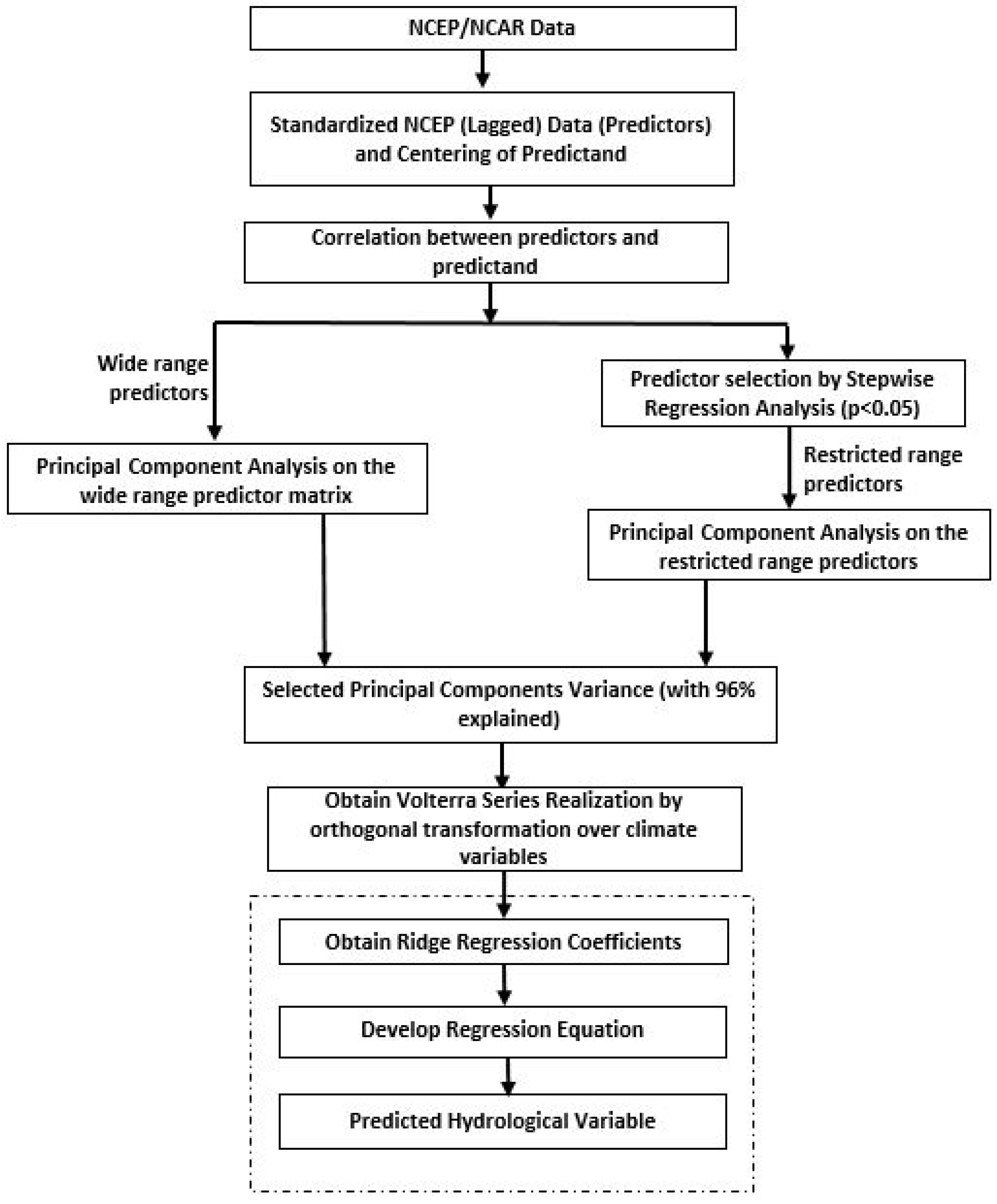
Figure 3 shows the overall schematic of the proposed downscaling model development methodology. The methodology is based on the concepts mentioned above in Section 3 (Tools and Techniques) of this paper. The developed model was used to downscale future rainfall at daily time intervals for the Palmerston North, Marton, Opiki, and Te Rehunga rainfall gauging stations, and the model was named the Statistical Downscaling Climate Classification with Ridge Regression (SDC2R2). The purpose of the proposed model is to deal with climate perturbation and produce successful rainfall predictions, on a daily basis. Previously, Ghosh and Mujumdar (2006) projected monthly rainfall with 90% accuracy by using PCA, fuzzy clustering and MLA [21]. In statistical downscaling, predictors play a crucial role but often suffer from multi-collinearity problems, thus, this study used PCA to deal with multi-collinearity and also to incorporate the temporal and spatial variability of a region, which is similar to the study of [13]. Further, the PCs were clustered by using fuzzy c-means clustering, which produced membership functions. Bas et al. (2019) transformed the membership function with various non-linear transformations and used ridge regression to deal with the multi-collinearity, which altogether improved the prediction results [22]. Thus, this study applied exponential and logarithmic transformations and finally combined them with ridge regression to produce successful daily rainfall projections. The statistical downscaling model developed by Singh et al. (2023) was capable of downscaling the daily rainfall with reasonable accuracy [9], but the model did not incorporate the frequency changes of the circulation types. Thus, the motivation behind the development of the SDC2R2 model is to involve the temporal variations of the atmospheric circulation in the downscaling model. This section provides a detailed description of each step used in the development of the statistical downscaling model (SDC2R2), as given in the following steps.

4.1. Step 1: Normalization

Pre-processing of the large-scale atmospheric data is required prior to training the statistical downscaling model, which includes standardization and normalization. Standardization is used to avoid the systematic biases from the mean and variance of NCEP and GCM predictors. Furthermore, normalization is the process of database design, which reduces data redundancy and eliminates undesirable characteristics. The usual process of obtaining the normalized data is by first subtracting the mean and then dividing by the standard deviation of the predictor variable, for a predefined baseline period for NCEP and GCM data. Additionally, Raje and Mujumdar (2009) mentioned that normalization is used as a predecessor to using Principal Component Analysis (PCA) [47].

4.2. Step 2: Selection of Predictors

In past downscaling studies, the selection of predictors is based on their relevant relationship with rainfall and availability in the climate models such as NCEP and GCM outputs [48].
The predictors selected for GCM grid points should assimilate the climate change signals and establish a valid relationship between predictors and predictand, even outside the calibration period. The chosen predictors were divided into two slices, the first slice (1961–1990) of Palmerston, (1965–1995) Marton, (1965–1995) Opiki, and (1961–1990) Te Rehunga rainfall gauging stations data was used for model calibration. However, the second slice (1991–2000) of Palmerston, (1995–2005) Marton, (1995–2005) Opiki, and (1991–2000) Te Rehunga rainfall gauging station data was used for the model validation. As mentioned by the National Institute of Water and Atmospheric Research (NIWA), the simulations with GCM predictors should be compared with the observed baseline/current climate data [49]. Thus, the rainfall data used in the present study to represent the current climate/baseline is from (2005–2020) Palmerston, (2005–2016) Marton, (2005–2019) Opiki and Te Rehunga. The baseline data is also used to compare the future projections.

4.3. Step 3: Classification for Climate Predictors for Regression Analysis

The MRA is most widely used in regression analysis. It is expressed by fitting the linear equation between the climate variables (predictors) and the response variable (predictand as rainfall). Despite its successful applications, the regression approach often struggles with difficulties due to the correlation among independent variables [40]. PCA is the standard approach of reducing the dimension and removing multicollinearity from the predictors. Thus, after selecting the potential predictors, the PCA was applied to obtain the principal components ( P C k t ) .
Although, there is no specific rule of selecting number of principal components, the Kaiser’s rule was adopted by Kannan and Ghosh (2013) for selection of the principal components. According to the Kaiser rule, all those components which explain variance less than 1% of the total data set are not used further in the analysis [49]. Thus, the study selected the number of principal components serving more than the 96% of total variance. The earlier study of Ghosh and Mujumdar (2006) used FCM technique to cluster principal components to downscale monthly rainfall and resulted with very high accuracy (90%) [21]. Thus, in this study, the principal components ( P C k t ) were clustered using the FCM technique and the membership values were calculated as μ i t   ( i = 1 , . . 3 ; t = 1 , k ) . Initially, to begin with the fuzzy clustering, the number of clusters were chosen randomly, and after few iterations, the optimal number of clusters were chosen as three, which was also similar to the study of Ghosh and Mujumdar (2006). The regression function for the clustered principal components were constituted as given below:
Y = X β R + ε
Y = y 1 y 2 y t ,
where Y is the target output (Equation (4)), X is the input matrix of the explanatory variables, and β R are the ridge regression coefficients, which could be obtained by means of the equations (Equations (5)) and (6)) discussed in the following section:

4.4. Step 4: Applying Transformation of Membership Values

Based on the distance between the cluster centre and the data point, the fuzzy c-means (FCM) clustering assigns membership to each data point of the clusters. Celikyilmaz and Turksen (2009) indicated that the logarithmic and the exponential transformation of the membership functions might increase the performance of the system [50]. Therefore, this study applied the exponential transformation of the membership values as given below:
X = μ i 1 e x p μ i 1 P C 11 P C k 1 μ i 2 e x p μ i 2 P C 12 P C k 2 μ i t e x p μ i t P C 1 t P C k t ,   i = 1 ,   ,   3
β R = X X + k I 1 X Y
Furthermore, PCA has widely being used to detect the spatial and temporal variations of rainfall over a region [51]. Gadgil and Iyengar (1980) mentioned that “the rainfall at any station n-thin the j-th year is expressed as the sum of the products of the coefficients,   A k n varying over space, associated with a temporal pattern or eigen vectors B t j ” [52] as given below:
R ( n , j ) = k = 1 t A k n × B t j

4.5. Step 4: Explanatory Variables Used as Orthogonal Filters

Additionally, as mentioned above, the temporal rainfall pattern represented by the eigen vectors are derived from the principal components. Thus, from Equations (5) and (7), the eigen vectors B n j will be replaced by P C k t . Additionally, the study applied the model with the assumption that, with respect to all principal components, the associated coefficient value is constant for a particular station. Thus, the matrix X of explanatory variables will be as given below:
X ^ = μ i 1 e x p μ i 1 k = 1 t A k × P C 11 +   P C k 1 μ i 2 e x p μ i 2 k = 1 t A k × P C 12 +   P C k 2 μ i t e x p μ i t k = 1 t A k × P C 1 t +   P C k t ,   i = 1 ,   ,   3
Furthermore, as mentioned in Step 3, the spatially varied coefficient A k value, which will be constant for all other P C k t   is derived by regressing the observed rainfall data over transformed matrix. Similar, to Equation (2), the transformed matrix is derived as the realization of the Volterra series expansion. Sequentially, the principal components were multiplied by the matrix of climate data (PRED) as given below:
Z 1,2 t = P R E D × P C 1,2 t
After running of various trials, the most suitable Z t value was obtained from Equation (9) and further the same value is used to obtain the principal component’s coefficient (constant value) from the equation given below:
A k = Z 1 . . . t Z 1 . . . t + k I 1 Z 1 . . . t Y
Additionally, the derived (principal component’s) coefficient value was used to obtain the final matrix of explanatory variables from Equation (8). Furthermore, this explanatory variable matrix was used as orthogonal filter to obtain the Volterra series realization as given below:
Z f = P R E D × X ^

4.6. Step 4: Calculated Fuzzy Ridge Regression Coefficient

As mentioned in Section 3.7 of this paper, the fuzzy ridge regression coefficient will be used to obtain future rainfall simulations. Thus, transformed matrix, Z f obtained from the above step was used to calculate the final values of fuzzy ridge regression coefficients from Equation (12) as shown here:
β R ^ =   Z f Z f + k I 1 Z f Y

4.7. Step 5: Rainfall Projections Using GCM Simulations

The careful selection of the predictor domain and the number of grids is critical in statistical downscaling. For instance, Najafi et al. (2011) [49] chose multiple GCM grids across the catchment, while Hassan et al. (2014) selected two GCM grids [50]. In this context, Kannan and Ghosh (2011) mentioned that the chosen statistical downscaling technique and the study area under investigation influence the chosen set of predictor domains. Therefore, the GCM grid selection may range from a single GCM grid to multiple GCM grids. Thus, this study selected a single grid of 4 GCMs for the chosen study area under investigation, shown in Figure 1. Additionally, the study derived future rainfall projections for the Representative Concentration Pathways (RCP) climate scenarios: RCP 2.5, RCP 4.5 and RCP 8.5 of CanESM2, which are based on radiative forcings. These RCPs range from low (RCP 2.5) to high (RCP 8.5) and are used to understand how climate change will affect the future, due to changes in the concentration of greenhouse gases [53].
The statistical relationship was established using NCEP reanalysis data as predictors and observed rainfall as the predictand. The same predictor set was extracted from the respective RCPs, and the established relationship was then applied to the predictors of 4 GCMs. Further, the methodology mentioned in above steps were used for modelling future rainfall for the study area.

4.8. Step 6: Bias Correction

The fuzzy ridge estimate deviates from the true value because of the bias problem [53]. However, Salvi et al. (2016) mentioned that with the introduction of fuzziness, the GCM predictors cannot be used directly due to the presence of bias with respect to reanalysis data [54], but Maraun et al. (2010) adjusted and improved simulated rainfall series for the bias correction, which was obtained from the statistical downscaling model [55]. Chim et al. (2020) used linear scaling bias correction method in their study and produced very good downscaling results, thus, we applied the linear scaling method to remove biasedness from the results of large-scale climate predictors [31]. Thus, the study proceeded with the bias correction process to tune downscaling predictions.

5. Performance Indices

The principal consideration of the SDC2R2 model is to downscale future rainfall having perturbations due to climate change impact. The performance indices used to access the efficiency of downscaling method SDC2R2 were the Normalized Root mean square error (NRMSE) and the Normalized Mean Absolute Error (NMAE), which are normalized to a scale [0, 1]. The normalization helps in simplifying the process of model performance comparison across different stations [25] and Coefficient of Determination ( R 2 ). The definition of RMSE, MAE and R2 are as defined below:
(i).
The expression for RMSE is:
RMSE = 1 n i 1 n O i P i 2
(ii).
The expression for MAE is:
MAE = 1 n i = 1 n O i P i
Normalized Root Mean Square Error (NRMSE) and Normalized Mean Absolute Error (NMAE) are expressed as follows:
NRMSE = RMSE/Range and NMAE = MAE/Range
where Range is the difference between the maximum and minimum value of the observed dataset.
(iii)
Coefficient of Determination ( R 2 ) is expressed as given below:
R 2 = i = 0 n P i n O ¯ 2 i = 0 n O i n O ¯ 2
where O i and P i are the observed and simulated rainfall data respectively for ‘n’ number of data points, O ¯ is the mean of the observed rainfall and P ¯ is the mean of simulated rainfall. The NRMSE and NMAE performance is observed to be better if the model evaluator value is closer to 0 whereas the R 2 value lies between [0, 1], and higher values indicate that the simulated results are more accurate.

6. Results and Discussion

The efficacy of the proposed SDC2R2 model was investigated by sequential application of the steps developed under the methodology section. The results obtained by the classification of climate change signals were to improve the closeness between the simulated and observed rainfall data by successfully incorporating the spatial and temporal variability intervals, to analyse future performance of rainfall projections due to the climate change impact. The proposed model was calibrated and validated at all four different stations of the Manawatu River basin to check its capability of producing appropriate results.

6.1. Performance of SDSM and SDCRR

The results obtained with SDSM and SDCRR are presented in Table 1, and show the performance of two models in terms of downscaling daily rainfall projections. The detailed comparison of the performance of the two models assisted in the selection of the base model. SDSM was used as a benchmark for comparing the performance of the proposed model, SDC2R2. The predictors used for SDSM modelling were selected by performing the correlation analysis between the predictors and predictand in SDSM. The best correlation results were improved by lagging predictors by 1 day. Based on the correlation results, the SDSM model was calibrated by using the predictors, namely the mean sea level pressure, the divergence near the surface, the geostrophic air flow velocity at 500 hPa, and the meridional velocity component at 500 hPa.
The statistical relationship was developed between these predictors and predictand to derive the future rainfall projections. The goodness of fit (R2) value obtained with the simulated series of daily rainfall for Palmerston, Marton, Opiki, and Te Rehunga was 0.28, 0.22, 0.31 and 0.25, respectively, as shown in Table 1. Additionally, the derived R 2 value of SDSM is lower but is comparable, as noted in the literature which has obtained even lower values of R 2 [30,41].
The   R 2 value demonstrated (Table 1) that for the daily rainfall event, the SDCRR model performed better than SDSM, thus will be used as a base model for the performance comparison of the proposed model. Furthermore, the SDC2R2 model was calibrated by using the most relevant predictor set, which was selected from the study of Singh et al. (2023) as mentioned in Section 2, shown in Table 2. The selected predictors could capture the regional variability very well and, thus, were used here to obtain the principal components for the SDC2R2 model.
Then, these principal components were used as orthogonal filters to develop the Volterra series realization. Finally, the transformed series was used to obtain the ridge regression coefficients. The goodness of fit ( R 2 ) values obtained for the Palmerston, Marton, Opiki, and Te Rehunga stations were 0.66, 0.75, 0.6, and 0.52, respectively, as shown in Table 3. The table shows that the performance of the SDCRR model is capable of simulating daily rainfall with optimum accuracy. The detailed working of the model is explained in [9]. The research also confirms that the SDCRR performed better than SDSM, in terms of simulating daily rainfall, and the same could be confirmed from Table 1 and Table 3.

6.2. Identifying Predictors for SDC2R2 Model

Table 2 presents the WR predictors influential in acquiring the minimum correlation coefficient value (r 1.5 ) at Palmerston, Marton, Opiki, and Te Rehunga. The reanalysis (NCEP) data is available at 500 and 850 pressure levels. It can be seen in Table 2 that there are many predictors, which are common at all four stations (shown in bold) and few of them (shown in italics) are effective, at either two or three stations. Among them, the mean sea level, wind speed, and vorticity of surface pressure level are commonly selected at all four stations. Then, the geopotential height available at 500 pressure level is selected at all four stations, whereas the same predictor at 850 pressure level is commonly selected at three stations (Palmerston, Marton, and Opiki) but not at Te Rehunga. Similarly, vorticity at 850 pressure level is linked well with the observed data of all four stations, but the same predictor at 500 pressure level was not correlated well only at the Te Rehunga station. Furthermore, the chosen set of predictors: 20 (Palmerston), 19 (Marton), 21 (Opiki), and 16 (Te Rehunga), shown in Table 2, are used to derive the principal components (PCs). The principal components retain the most valuable part of all input variables in the form of explained variance. The number of PCs was selected to meet the requirement of the percent of variance to be accounted for in the regression analysis, as mentioned in the methodology. It is essential for the selected number of PCs to serve more than the average amount of total variance.
The study selected 12 (Palmerston), 11 (Marton), 12 (Opiki), and 10 (Te Rehunga) PCs at these stations, to explain 96% of the total variance of the original climate predictors. The chosen principal components were clustered to develop the explanation, as mentioned in Section 4 (model development). These membership functions will be used for the ridge regression analysis.

6.3. Performance of the SDC2R2 Model over the Calibration and Validation Period

The model was calibrated and validated for the daily rainfall data at the four stations. The SDC2R2 model performed well at each station. As observed from Table 3, the calibration of the SDC2R2 model provided R 2 of 0.78, 0.74, 0.77, and 0.72 for Palmerston, Marton, Opiki, and Te Rehunga stations, respectively.
The goodness of fit (R2) value obtained with SDC2R2 is higher than those of SDCRR at all four stations, Palmerston, Opiki, Marton, and Te Rehunga, which assures that the model produced better daily rainfall simulations than SDCRR. The SDC2R2 model produced successful daily rainfall projections from large-scale climate variables by capturing non-linear interactions of the climate variables. The performance of the model was improved with the classification of climate variables to derive membership functions with clustered principal components, used to incorporate climate change in terms of temporal and spatial variability by statistical downscaling.
Furthermore, the consistency of the results was maintained during the validation period, with R 2 values of 0.88, 0.81, 0.84, and 0.76 for all four stations namely, Palmerston, Marton, Opiki and Te Rehunga. The results obtained with other performance indices, such as NRMSE and NMAE, were very good at all four stations. Table 4 shows that the model performance is highly satisfactory, as the NRMSE and NMAE values are close to zero. As mentioned in Section 5, if the value of NRMSE and NMAE is low, then it is an indication that the downscaled values have higher similarity to the observed data. Thus, the results obtained with the satisfactory estimates of all performance indices, indicated that the model responded in an effective manner to the daily rainfall data.

6.4. Application of Bias Correction to the SDC2R2 Model

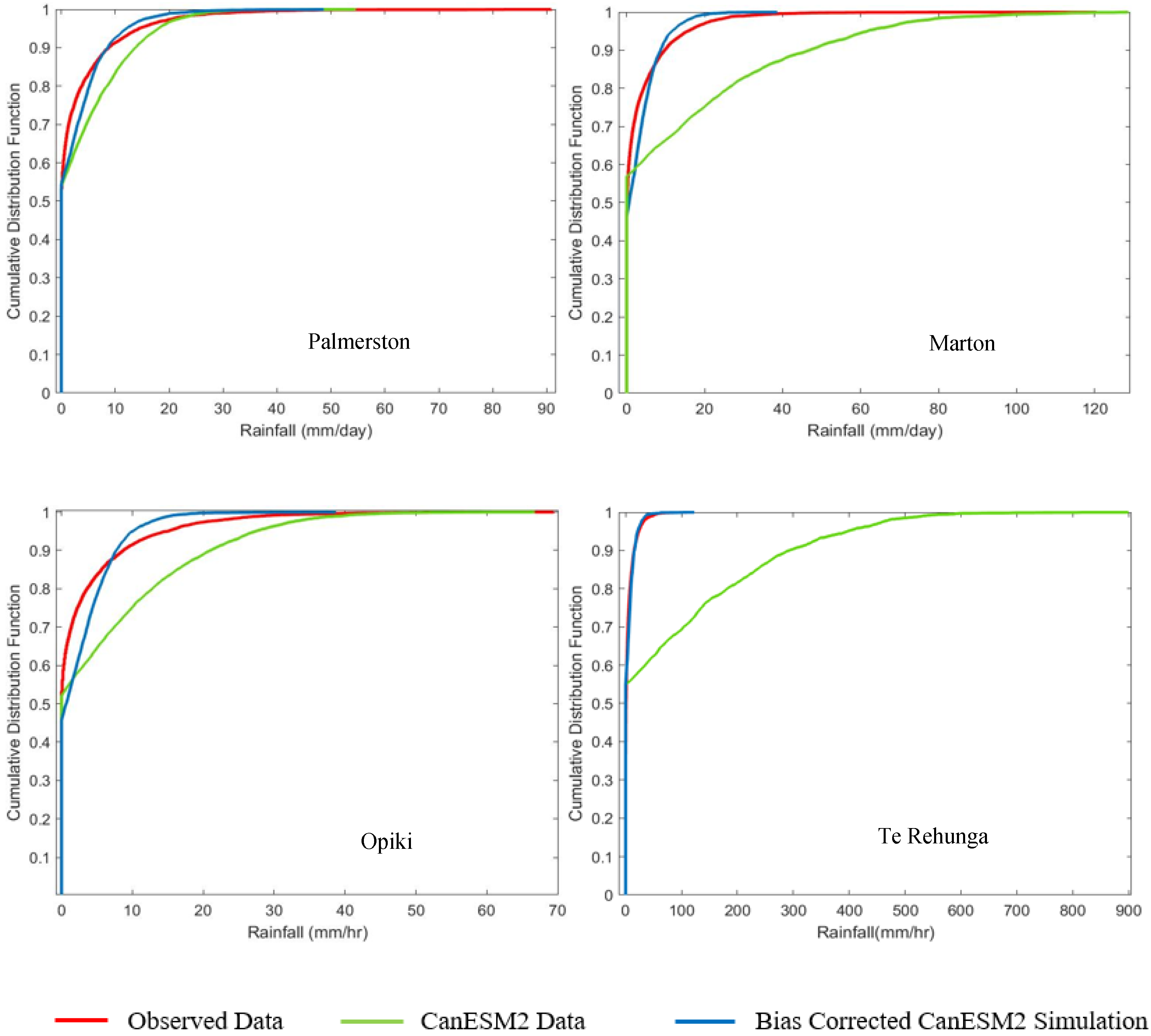
Results obtained in Table 3 and Table 4 show that the proposed model performed well at all the stations with the reanalysis (NCEP) climate data. On the contrary, when the ability of the SDC2R2 model was tested by using the historical predictor variables of GCM (CanESM2) data, the results (see Figure 4) indicated that the downscaling of daily rainfall values were not satisfactory due to the introduction of fuzziness.
Thus, a bias correction (linear scaling method) was used in this study to improve the simulation by assuming the factors obtained by the correction method will be stationary. The bias factors were obtained by applying the linear scaling algorithm for the rainfall simulated with CanESM2 (historical) data and the same factors were used for the future rainfall scenarios. Figure 4 compares the cumulative distribution function (CDF) of the simulated rainfall series generated at each station with the observed rainfall data. The CDF of simulated rainfall was obtained by using the bias-corrected rainfall simulation obtained with historical CanESM2 GCM predictors (1985–2005) and observed data of the same time period. The figure clearly shows that the bias-corrected rainfall simulation is showing minimum deviation from the observed data.
Figure 5 shows the comparison between observed data and bias-corrected simulated rainfall. The SDC2R2 model performed well for the daily rainfall data at Palmerston, Marton, Opiki, and Te Rehunga stations by using the CanESM2 GCM historical predictors. Another important observation is that the SDC2R2 model is able to capture the percent of dry days (rainfall < 1   mm/day) as well as wet days (rainfall 1 mm/day) adequately. The model was able to capture about 55% of dry days at Palmerston and Te Rehunga, whereas 48% of dry days at Marton and Opiki, which is equal to the actual observed dry day percent at respective stations (Figure 5).
Figure 5 shows that the model was able to capture the wet days (greater than 20 mm/day), as both simulated and observed curves showed optimum closeness at Te Rehunga followed by Palmerston, Marton, and Opiki.
Additionally, in terms of capturing extreme events (maximum rainfall), the model performed well at both Te Rehunga and Palmerston stations. At other stations, the model did not perform well in capturing maximum rainfall but responded well to minimum rainfall, which ensures that the developed model could be used for both flood and drought studies.

6.5. Future Projections Using GCM Simulations

This study investigated climate change impact over the future period 2031–2060 under different emission scenarios of RCPs. Chim et al. (2020) [31] utilized these emission scenarios, and the findings indicate a strong likelihood of decreased precipitation across all future scenarios for the Cambodia catchment. Similarly, Mishra and Lihare [56] projected that the precipitation is expected to change significantly under future climate conditions in most river basins across the Indian subcontinent. Projections indicate that precipitation could increase by up to 14%, 30%, and 50% in the Near, Mid, and End-term climates, under the RCP 4.5 and 8.5 scenarios.
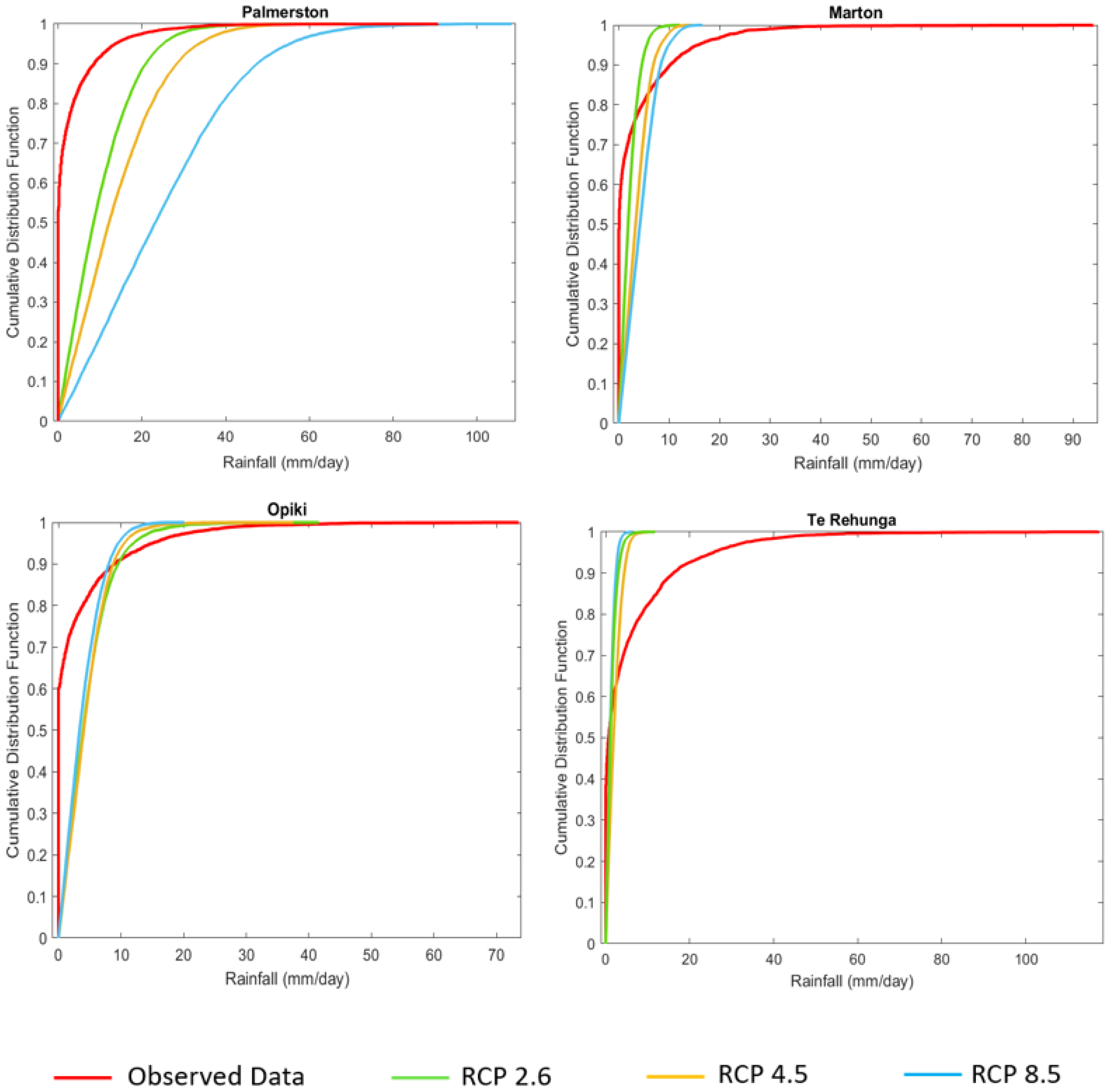
The CDF of future rainfall projections at daily time steps obtained at the four downscaling stations are shown in Figure 6. Although the rainfall event properties can be measured by many methods, the CDFs are used as the best tool to determine the downscaling model’s (SDC2R2) ability. The change in frequency of low and high rainfall is recorded with the shift in CDFs above and below the observed rainfall curve [49].
The developed model SDC2R2, based on ridge regression and fuzzy clustering, is applied to downscale daily rainfall for the future period of 2031–2060 and compared to the base period observed rainfall; 2005–2020 for Palmerston, 2005–2019 for Opiki and Te Rehunga, and 2005–2016 for Marton. The CDFs obtained for three scenarios showed wide variation in the future rainfall projections at Palmerston, Marton, Opiki, and Te Rehunga rain stations. At Palmerston, there is a downward shift in CDF (refer to Figure 6), which indicates that in comparison to the baseline data, the probability of obtaining high rainfall frequency for the future (2031–2060) is higher with all three scenarios, RCP 2.6, RCP 4.5, and RCP 8.5. Alternatively, CDF plotted at Te Rehunga shows minimal instances of receiving low to medium rainfall values when compared with the observed data (see Figure 6). Additionally, Opiki and Marton are expected to receive low instances of rainfall under the influence of all three scenarios (RCP 2.6, RCP 4.5, and RCP 8.5) in comparison to the observed rainfall (refer to Figure 6).

7. Conclusions

This paper evaluates the fuzzy function approach combined with a regression model to produce successful daily rainfall projections from large-scale climate variables for the Manawatu catchment, New Zealand. The modelling framework was applied to four different stations, spanning the study area, and its performance was evaluated at each station. PCA and fuzzy clustering were performed to improve the model performance in terms of capturing the temporal and spatial variability. Another important step was that the membership functions were transformed into exponential transformation and the explanatory matrix was formed by combining membership functions, transformed membership functions, and principal components. This explanatory matrix was used to obtain the transformation of climate predictors in the form of Volterra series expansion. The transformed climate predictors were used to regress the observed data by using ridge regression analysis, which added value to the performance of the model. Additionally, the explanatory variable matrix was formed by the combination of membership functions, and principal components, where principal components were assumed to have a constant coefficient value. As the model is a combination of regression and classification, it can thus be considered a hybrid model of weather typing and transfer function. Furthermore, the performance of the SDC2R2 model was compared with SDCRR and SDSM. Singh et al. (2023) indicated that the SDCRR performed better in simulating daily rainfall than SDSM, which is widely used in various studies for downscaling rainfall (Osman and Abdellatif, 2016; Hashmi et al., 2009) [57,58] The results of this study show that the SDC2R2 model simulated daily rainfall with higher accuracy than that of SDCRR. Based on the results obtained from the Palmerston, Marton, Opiki, and Te Rehunga stations, it is concluded that the proposed model, SDC2R2, was able to simulate the daily rainfall with optimum accuracy at each station. The bias problem of the fuzzy ridge estimator was also addressed by applying linear scaling at the end of downscaling. The methodology developed could be used to examine hydrologic implications due to climate change. Further, it is worth obtaining future projections with different GCMs, so the dependence on a single GCM result is avoided, which could further lead to appropriate planning. Thus, working with multiple GCMs in SDC2R2, in terms of capturing GCM uncertainty, is proposed to be carried out in future research. Future research could also include a comparison of various non-stationarity trends in rainfall data based on projections from multiple GCMs.

Author Contributions

Conceptualization, P.S.; methodology, P.S.; formal analysis, P.S.; investigation, P.S.; data curation, P.S. and writing—original draft preparation, P.S.; writing—review and editing, P.S. and A.Y.S.; supervision, A.Y.S., B.W.M. and L.W. All authors have read and agreed to the published version of the manuscript.

Funding

This research received no external funding.

Data Availability Statement

The developed computer codes for downscaling daily rainfall with the SDC2R2 model are available on request from the authors.

Acknowledgments

The authors express their gratitude to the Horizons Regional Council for supplying the rainfall data. They also thank the National Climate Database (http://cliflo.niwa.co.nz/, 1 January 2021) and Environment and Climate Change Canada (ECCC) (Canadian site http://climate-scenarios.canada.ca/, 1 January 2021) for providing access to their websites to extract the respective data.

Conflicts of Interest

The authors declare no conflict of interest.

References

  1. Tahir, T.; Hashim, A.M.; Yusof, K.W. Statistical Downscaling of Rainfall under Transitional Climate in Limbang River Basin by Using SDSM. IOP Conf. Ser. Earth Environ. Sci. 2018, 140, 012037. [Google Scholar] [CrossRef]
  2. Singh, S.; Kannan, S.; Timbadiya, P.V. Statistical Downscaling of Multisite Daily Precipitation for Tapi Basin Using Kernel Regression Model. Curr. Sci. 2016, 110, 1468–1484. [Google Scholar]
  3. Munawar, S.; Rahman, G.; Farhan, M.; Moazzam, U.; Miandad, M.; Ullah, K.; Al-ansari, N.; Thi, N.; Linh, T. Future Climate Projections Using SDSM and LARS-WG Downscaling Methods for CMIP5 GCMs over the Transboundary Jhelum River Basin of the Himalayas Region. Atmosphere 2022, 13, 898. [Google Scholar] [CrossRef]
  4. Ali, S.; Eum, H.; Cho, J.; Dan, L.; Khan, F.; Dairaku, K.; Shrestha, M.L.; Hwang, S.; Nasim, W.; Khan, I.A.; et al. Assessment of Climate Extremes in Future Projections Downscaled by Multiple Statistical Downscaling Methods over Pakistan. Atmos. Res. 2019, 222, 114–133. [Google Scholar] [CrossRef]
  5. Hashmi, M.Z.; Shamseldin, A.Y.; Melville, B.W. Statistical Downscaling of Precipitation: State-of-the-Art and Application of Bayesian Multi-Model Approach for Uncertainty Assessment. Hydrol. Earth Syst. Sci. Discuss. 2009, 6, 6535–6579. [Google Scholar] [CrossRef]
  6. Devak, M.; Dhanya, C.T. Downscaling of Precipitation in Mahanadi Basin, India. Int. J. Civ. Eng. Res. 2014, 5, 111–120. [Google Scholar]
  7. Salvi, K.; Ghosh, S. High-Resolution Multisite Daily Rainfall Projections in India with Statistical Downscaling for Climate Change Impacts Assessment. J. Geophys. Res. Atmos. 2013, 118, 3557–3578. [Google Scholar] [CrossRef]
  8. Wetterhall, F. Statistical Downscaling of Precipitation from Large-Scale Atmospheric Circulation. Ph.D. Thesis, Uppala University, Uppsala, Sweden, 2005. Available online: https://www.researchgate.net/publication/260265285_Statistical_Downscaling_of_Precipitation_from_Large scale_Atmospheric_Circulation (accessed on 1 January 2021).
  9. Singh, P.; Shamseldin, A.Y.; Melville, B.W.; Wotherspoon, L. Development of Statistical Downscaling Model Based on Volterra Series Realization, Principal Components and Ridge Regression. Model. Earth Syst. Environ. 2023, 9, 3361–3380. [Google Scholar] [CrossRef]
  10. Ghosh, S.; Mujumdar, P.P. Statistical Downscaling of GCM Simulations to Streamflow Using Relevance Vector Machine. Adv. Water Resour. 2008, 31, 132–146. [Google Scholar] [CrossRef]
  11. Govindaraju, R.S. Bayesian Learning and Relevance Vector Machines for Hydrologic Applications. In Proceedings of the 2nd Indian International Conference on Artificial Intelligence IICAI 2005, Pune, India, 20–22 December 2005; pp. 1078–1093. Available online: https://www.researchgate.net/publication/220887942_Bayesian_Learning_and_Relevance_Vector_Machines_for_Hydrologic_Applications_keynote_speech_of_the_session (accessed on 1 January 2021).
  12. Lakhanpal, A.; Sehgal, V.; Maheswaran, R.; Khosa, R.; Sridhar, V. A Non-Linear and Non-Stationary Perspective for Downscaling Mean Monthly Temperature: A Wavelet Coupled Second Order Volterra Model. Stoch. Environ. Res. Risk Assess. 2017, 31, 2159–2181. [Google Scholar] [CrossRef]
  13. Machiwal, D.; Kumar, S.; Meena, H.M.; Santra, P.; Singh, R.K.; Singh, D.V. Clustering of Rainfall Stations and Distinguishing Influential Factors Using PCA and HCA Techniques over the Western Dry Region of India. Meteorol. Appl. 2019, 26, 300–311. [Google Scholar] [CrossRef]
  14. Suhaila, J.; Jemain, A.A. A Comparison of the Rainfall Patterns between Stations on the East and the West Coasts of Peninsular Malaysia Using the Smoothing Model of Rainfall Amounts. Meteorol. Appl. 2009, 16, 391–401. [Google Scholar] [CrossRef]
  15. Sabziparvar, A.A.; Movahedi, S.; Asakereh, H.; Maryanaji, Z.; Masoodian, S.A. Geographical Factors Affecting Variability of Precipitation Regime in Iran. Theor. Appl. Climatol. 2015, 120, 367–376. [Google Scholar] [CrossRef]
  16. Gupta, A.; Kamble, T.; Machiwal, D. Comparison of Ordinary and Bayesian Kriging Techniques in Depicting Rainfall Variability in Arid and Semi-Arid Regions of North-West India. Environ. Earth Sci. 2017, 76, 512. [Google Scholar] [CrossRef]
  17. Machiwal, D.; Dayal, D.; Kumar, S. Long-Term Rainfall Trends and Change Points in Hot and Cold Arid Regions of India. Hydrol. Sci. J. 2017, 62, 1050–1066. [Google Scholar] [CrossRef]
  18. Medina-Cobo, M.T.; García-Marín, A.P.; Estévez, J.; Jiménez-Hornero, F.J.; Ayuso-Muñoz, J.L. Obtaining Homogeneous Regions by Determining the Generalized Fractal Dimensions of Validated Daily Rainfall Data Sets. Water Resour. Manag. 2017, 31, 2333–2348. [Google Scholar] [CrossRef]
  19. Lin, F.R.; Wu, N.J.; Tsay, T.K. Applications of Cluster Analysis and Pattern Recognition for Typhoon Hourly Rainfall Forecast. Adv. Meteorol. 2017, 2017, 5019646. [Google Scholar] [CrossRef]
  20. Amissah-Arthur, A.; Jagtap, S.S. Geographic Variation in Growing Season Rainfall during Three Decades in Nigeria Using Principal Component and Cluster Analyses. Theor. Appl. Climatol. 1999, 63, 107–116. [Google Scholar] [CrossRef]
  21. Ghosh, S.; Mujumdar, P.P. Future rainfall scenario over Orissa with GCM projections by statistical downscaling. Curr. Sci. 2006, 90, 396–404. [Google Scholar]
  22. Bas, E.; Egrioglu, E.; Yolcu, U.; Grosan, C. Type 1 Fuzzy Function Approach Based on Ridge Regression for Forecasting. Granul. Comput. 2019, 4, 629–637. [Google Scholar] [CrossRef]
  23. Watanabe, A. The Volterra Series Expansion of Functionals Defined on the Finite-dimensional Vector Space and Its Application to Saving of Computational Effort for Volterra Kernels. Electron. Commun. Jpn. 1986, 69, 37–46. [Google Scholar] [CrossRef]
  24. Chou, C. ming Efficient Nonlinear Modeling of Rainfall-Runoff Process Using Wavelet Compression. J. Hydrol. 2007, 332, 442–455. [Google Scholar] [CrossRef]
  25. Sehgal, V.; Lakhanpal, A.; Maheswaran, R.; Khosa, R.; Sridhar, V. Application of Multi-Scale Wavelet Entropy and Multi-Resolution Volterra Models for Climatic Downscaling. J. Hydrol. 2018, 556, 1078–1095. [Google Scholar] [CrossRef]
  26. Hoerl, A.E.; Kennard, R.W. American Society for Quality Ridge Regression : Biased Estimation for Nonorthogonal Problems. Technometrics 1970, 12, 55–67. [Google Scholar] [CrossRef]
  27. Eoerl, A.E.; Kaanard, R.W.; Baldwin, K.F. Ridge Regression: Some Simouxions. Commun. Stat. 1975, 4, 105–123. [Google Scholar] [CrossRef]
  28. Hermans, O.F. Flood Management in New Zealand: Exploring Management and Practice in Otago and the Manawatu. Ph.D. Thesis, University of Otago, Dunedin, New Zealand, 2017. [Google Scholar]
  29. Shashikanth, K.; Madhusoodhanan, C.G.; Ghosh, S.; Eldho, T.I.; Rajendran, K.; Murtugudde, R. Comparing Statistically Downscaled Simulations of Indian Monsoon at Different Spatial Resolutions. J. Hydrol. 2014, 519, 3163–3177. [Google Scholar] [CrossRef]
  30. Yang, C.; Wang, N.; Wang, S.; Zhou, L. Performance Comparison of Three Predictor Selection Methods for Statistical Downscaling of Daily Precipitation. Theor. Appl. Climatol. 2018, 131, 43–54. [Google Scholar] [CrossRef]
  31. Chim, K.; Tunnicliffe, J.; Shamseldin, A.; Chan, K. Identifying Future Climate Change and Drought Detection Using CanESM2 in the Upper Siem Reap River, Cambodia. Dyn. Atmos. Ocean. 2020, 94, 101182. [Google Scholar] [CrossRef]
  32. Rashid, M.M.; Beecham, S.; Chowdhury, R.K. Statistical Downscaling of Rainfall: A Non-Stationary and Multi-Resolution Approach. Theor. Appl. Climatol. 2016, 124, 919–933. [Google Scholar] [CrossRef]
  33. Agarwal, A.; Marwan, N.; Rathinasamy, M.; Merz, B.; Kurths, J. Multi-Scale Event Synchronization Analysis for Unravelling Climate Processes: A Wavelet-Based Approach. Nonlinear Process. Geophys. 2017, 24, 599–611. [Google Scholar] [CrossRef]
  34. Karim, S.A.A.; Kamsani, N.F. Fuzzy Multiple Linear Regression. In Water Quality Index Prediction Using Multiple Linear Fuzzy Regression Model: SpringerBriefs in Water Science and Technology; Springer: Singapore, 2020; pp. 11–21. [Google Scholar] [CrossRef]
  35. Wetterhall, F.; Bádossy, A.; Chen, D.; Halldin, S.; Xu, C.Y. Daily Precipitation-Downscaling Techniques in Three Chinese Regions. Water Resour. Res. 2006, 42, 1–13. [Google Scholar] [CrossRef]
  36. Zhang, Z.; Xu, C.; Huang, J.; Zhang, J.; Yao, J.; Wang, B. Estimation of Future Precipitation Change in the Yangtze River Basin by Using Statistical Downscaling Method. Stoch. Environ. Res. Risk Assess. 2010, 25, 781–792. [Google Scholar] [CrossRef]
  37. Williams, A.N. Diagnostic Evaluation in Aspirin-Exacerbated Respiratory Disease. Immunol. Allergy Clin. N. Am. 2016, 36, 657–668. [Google Scholar] [CrossRef]
  38. Rajab, J.M.; MatJafri, M.Z.; Lim, H.S. Combining Multiple Regression and Principal Component Analysis for Accurate Predictions for Column Ozone in Peninsular Malaysia. Atmos. Environ. 2013, 71, 36–43. [Google Scholar] [CrossRef]
  39. Rahman, A.S.; Rahman, A. Application of Principal Component Analysis and Cluster Analysis in Regional Flood Frequency Analysis: A Case Study in New South Wales, Australia. Water 2020, 12, 781. [Google Scholar] [CrossRef]
  40. Dogruparmak, S.C.; Keskin, G.A.; Yaman, S.; Alkan, A. Using Principal Component Analysis and Fuzzy C-Means Clustering for the Assessment of Air Quality Monitoring. Atmos. Pollut. Res. 2014, 5, 656–663. [Google Scholar] [CrossRef]
  41. Zhang, W.; Huang, T.; Chen, J. A Robust Bias-Correction Fuzzy Weighted C-Ordered-Means Clustering Algorithm. Math. Probl. Eng. 2019, 2019, 5984649. [Google Scholar] [CrossRef]
  42. Engineering, H. Downscaling from GCMs to Local Climate through Stochastic Andra s Ba Rdossy. J. Environ. Manag. 1997, 49, 7–17. [Google Scholar]
  43. Bardossy, A.; Duckstein, L.; Bogardi, I. Fuzzy Rule-based Classification of Atmospheric Circulation Patterns. Int. J. Climatol. 1995, 15, 1087–1097. [Google Scholar] [CrossRef]
  44. Bárdossy, A.; Pegram, G.; Sinclair, S.; Pringle, J.; Stretch, D. Circulation Patterns Identified by Spatial Rainfall and Ocean Wave Fields in Southern Africa. Front. Environ. Sci. 2015, 3, 31. [Google Scholar] [CrossRef]
  45. Raje, D.; Mujumdar, P.P. A Conditional Random Field-Based Downscaling Method for Assessment of Climate Change Impact on Multisite Daily Precipitation in the Mahanadi Basin. Water Resour. Res. 2009, 45, 1–20. [Google Scholar] [CrossRef]
  46. Pavan, Y.; Maheswaran, R.; Agarwal, A.; Sivakumar, B. Intercomparison of Downscaling Methods for Daily Precipitation with Emphasis on Wavelet-Based Hybrid Models. J. Hydrol. 2021, 599, 126373. [Google Scholar] [CrossRef]
  47. Najafi, M.R.; Moradkhani, H.; Wherry, S.A. Statistical Downscaling of Precipitation Using Machine Learning with Optimal Predictor Selection. J. Hydrol. Eng. 2011, 16, 650–664. [Google Scholar] [CrossRef]
  48. Hassan, Z.; Shamsudin, S.; Harun, S. Application of SDSM and LARS-WG for Simulating and Downscaling of Rainfall and Temperature. Theor. Appl. Climatol. 2014, 116, 243–257. [Google Scholar] [CrossRef]
  49. Kannan, S.; Ghosh, S. A Nonparametric Kernel Regression Model for Downscaling Multisite Daily Precipitation in the Mahanadi Basin. Water Resour. Res. 2013, 49, 1360–1385. [Google Scholar] [CrossRef]
  50. Celikyilmaz, A.; Türksen, I.B. Improved Fuzzy Clustering. Stud. Fuzziness Soft Comput. 2009, 240, 51–104. [Google Scholar] [CrossRef]
  51. Roy Bhowmik, S.K.; Sen Roy, S. Principal Component Analysis to Study Spatial Variability of Errors in the INSAT Derived Quantitative Precipitation Estimates over Indian Monsoon Region. Atmosfera 2006, 19, 255–265. [Google Scholar]
  52. Gadgil, S.; Narayana Iyengar, R. Cluster Analysis of Rainfall Stations of the Indian Peninsula. Q. J. R. Meteorol. Soc. 1980, 106, 873–886. [Google Scholar] [CrossRef]
  53. Rabiei, M.R.; Arashi, M.; Farrokhi, M. Fuzzy Ridge Regression with Fuzzy Input and Output. Soft Comput. 2019, 23, 12189–12198. [Google Scholar] [CrossRef]
  54. Salvi, K.; Ghosh, S.; Ganguly, A.R. Credibility of Statistical Downscaling under Nonstationary Climate; Springer: Berlin/Heidelberg, Germany, 2016; Volume 46, ISBN 0038201526. [Google Scholar]
  55. Maraun, D.; Brienen, S.; Rust, H.W.; Sauter, T.; Themeßl, M.; Venema, V.K.C.; Chun, K.P. Precipitation Downscaling under Climate Change: Recent developments to bridge the gap between dynamical models and the end user. Rev. Geophys. 2010, 48, 1–34. [Google Scholar] [CrossRef]
  56. Mishra, V.; Lihare, R. Hydrologic sensitivity of Indian sub-continental river basins to climate change. Glob. Planet. Chang. 2016, 139, 78–96. [Google Scholar] [CrossRef]
  57. Osman, Y.Z.; Abdellatif, M.E. Improving accuracy of downscaling rainfall by combining predictions of different statistical downscale models. Water Sci. 2016, 30, 61–75. [Google Scholar] [CrossRef]
  58. Hashmi, M.Z.; Shamseldin, A.Y.; Melville, B.W. Downscaling of Future Rainfall Extreme Events: A Weather Generator Based Approach. In Proceedings of the 18th World IMACS Congress MODSIM09 International Congress Modelling and Simulation, Cairns, Australia, 13–17 July 2009; pp. 3928–3934. [Google Scholar]
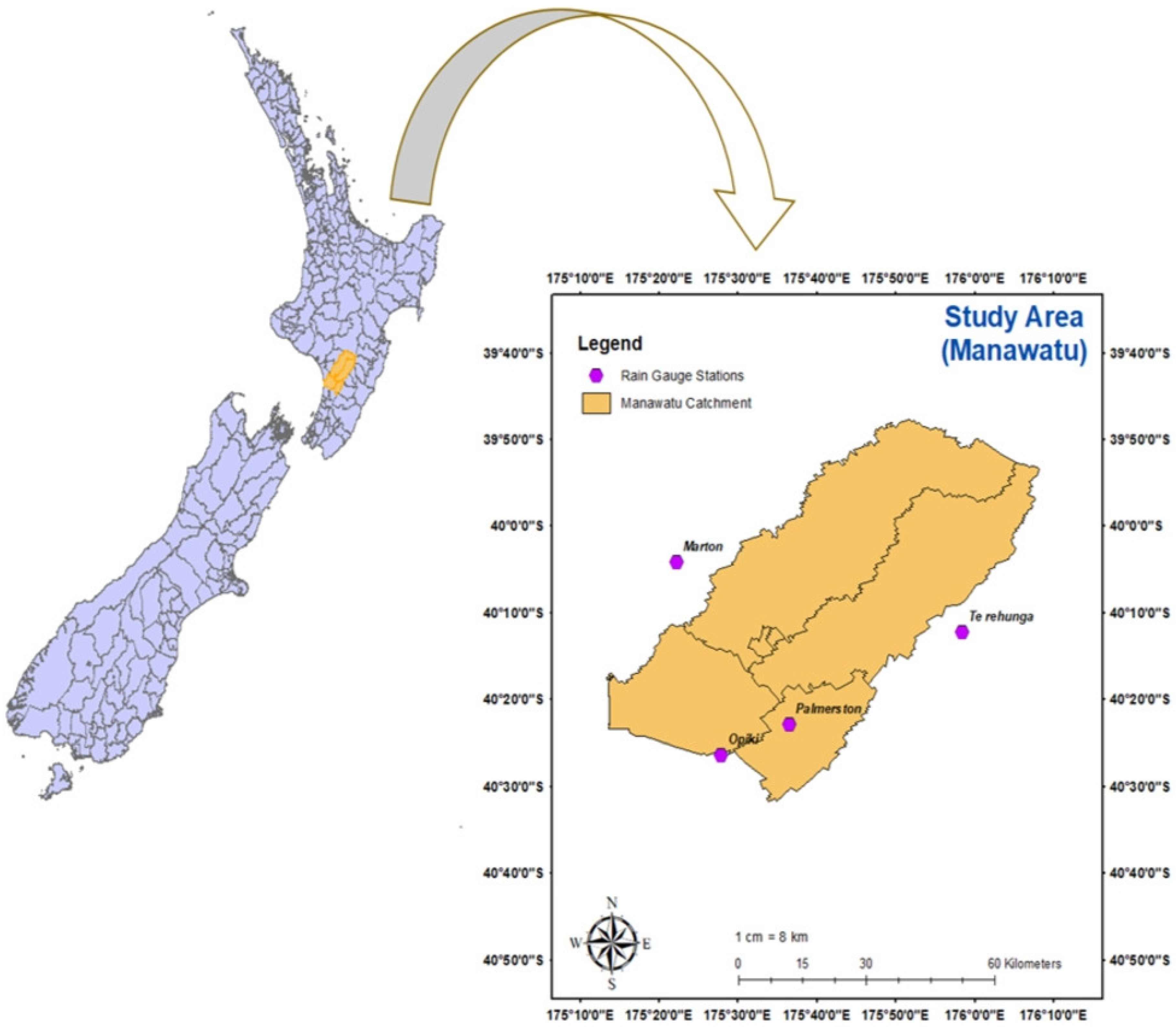
Figure 1. Location of the Manawatu Catchment.
Hydrology 11 00144 g001
Figure 2. Methodology of the SDCRR downscaling.
Hydrology 11 00144 g002
Figure 3. Flowchart of the proposed downscaling framework (SDC2R2).
Hydrology 11 00144 g003
Figure 4. Bias-corrected CDF of daily rainfall obtained by using the baseline CanESM2 historical (baseline) data (1985–2005) for Marton, Opiki and (1985–2001) for Palmerston and Te Rehunga Stations.
Hydrology 11 00144 g004
Figure 5. CDF of daily rainfall obtained from SDCRR downscaling model using the (baseline) CanESM2 historical data (1985–2005) for Marton, Opiki, and (1985–2001) for Palmerston and Te Rehunga Stations.
Hydrology 11 00144 g005
Figure 6. CDF of baseline/observed data (2005–2020) for Palmerston, (2005–2019) for Opiki and Te Rehunga, and (2005–2016) for Marton using CanESM2 predictor data under RCP 2.5, RCP 4.5 and RCP 8.5 scenarios compared with simulated future (2031–2060).
Hydrology 11 00144 g006
Table 1. Performance of SDSM.
Station NameModelYear LengthGoodness of Fit (R2) Obtained by SDSMGoodness of Fit (R2) Obtained by SDCRR
PalmerstonCalibration1961–19900.280.66
MartonCalibration1965–19950.220.75
OpikiCalibration1965–19950.310.82
TeRehungaCalibration1961–19900.250.76
Table 2. List of WR predictors used in the SDC2R2 model.
WR Predictors
LevelPalmerstonMartonOpikiTeRehunga
SurfaceMean sea level (mslp)Mean sea level pressure (mslp)Mean sea level (mslp)Mean sea level pressure (mslp)
Wind Speed (p_f)Wind Speed (p_f)Wind Speed (p_f)Wind Speed (p_f)
Vorticity (p_z)Vorticity (p_z)Vorticity (p_z)Vorticity (p_z)
Divergence of True Wind (p_zh)Divergence of True Wind (p_zh)Divergence of True Wind (p_zh)Divergence of True Wind (p_zh)
Total Precipitation (prcp)Total Precipitation (prcp)Total Precipitation (prcp)Total Precipitation (prcp)
Specific Humidity (shum)Specific Humidity (shum)Specific Humidity (shum)
Meridonal Wind Component (p_v)
500 hpaGeopotential Height (p500)Geopotential Height (p500)Geopotential Height (p500)Geopotential Height (p500)
Wind Speed (p5_f)Wind Speed (p5_f)Wind Speed (p5_f)Wind Speed (p5_f)
Zonal Wind Component (p5_u)Zonal Wind Component (p5_u)Zonal Wind Component (p5_u)Zonal Wind Component (p5_u)
Meridonal Wind Component (p5_v)Meridonal Wind Component (p5_v)Meridonal Wind Component (p5_v)Meridonal Wind Component (p5_v)
Vorticity (p5_z)Vorticity (p5_z)Vorticity (p5_z)Vorticity (p5_z)
Divergence of True Wind (p5_zh)Divergence of True Wind (p5_zh)Divergence of True Wind (p5_zh)
Specific Humidity (shum500)Specific Humidity (shum500)Specific Humidity (shum500)Specific Humidity (shum500)
850 hpaGeopotential Height (p850)Geopotential Height (p850)Geopotential Height (p850)Geopotential Height (p850)
Wind Speed (p8_f) Wind Speed (p8_f)Wind Speed (p8_f)
Zonal Wind Components (p8_u)Zonal Wind Components (p8_u)Zonal Wind Components (p8_u)
Vorticity (p8_z)Vorticity (p8_z)Vorticity (p8_z)Vorticity (p8_z)
Wind Direction (p8th)Wind Direction (p8th)Wind Direction (p8th)
Divergence of True Wind (p8_zh)Divergence of True Wind (p8_zh)Divergence of True Wind (p8_zh)Divergence of True Wind (p8_zh)
Specific Humidity (shum850)Specific Humidity (shum850)Specific Humidity (shum850)Specific Humidity (shum850)
Table 3. Performance of the SDC2R2 model at different rain gauge stations.
Station NameDownscaling ModelYear Length R 2
(SDCRR)
R 2
(SDC2R2)
PalmerstonCalibration1961–19900.660.78
Validation1991–20010.770.88
MartonCalibration1965–19950.740.84
Validation1996–20050.750.81
OpikiCalibration1965–19950.600.77
Validation1996–20050.820.84
TeRehungaCalibration1961–19900.520.72
Validation1991–20010.760.76
Table 4. Performance of the SDC2R2 model at different rain gauge stations.
Station NameSDCRR ModelYear LengthNRMSENMAE
PalmerstonCalibration1961–19900.0890.031
Validation1991–20010.1070.042
MartonCalibration1965–19950.0930.032
Validation1996–20050.0830.029
OpikiCalibration1965–19950.13950.055
Validation1996–20050.14410.055
TeRehungaCalibration1961–19900.10290.039
Validation1991–20010.09810.025
Disclaimer/Publisher’s Note: The statements, opinions and data contained in all publications are solely those of the individual author(s) and contributor(s) and not of MDPI and/or the editor(s). MDPI and/or the editor(s) disclaim responsibility for any injury to people or property resulting from any ideas, methods, instructions or products referred to in the content.