Article

Does Applying Subsampling in Quantile Mapping Affect the Climate Change Signal?

1
Research Institute for Forest Ecology and Forestry Rhineland-Palatinate, 67705 Trippstadt, Germany
2
Department of Physical Geography, University of Trier, 54286 Trier, Germany
*
Author to whom correspondence should be addressed.
Hydrology 2024, 11(9), 143; https://doi.org/10.3390/hydrology11090143
Submission received: 2 August 2024 / Revised: 4 September 2024 / Accepted: 6 September 2024 / Published: 9 September 2024

Abstract

:
Bias in regional climate model (RCM) data makes bias correction (BC) a necessary pre-processing step in climate change impact studies. Among a variety of different BC methods, quantile mapping (QM) is a popular and powerful BC method. Studies have shown that QM may be vulnerable to reductions in calibration sample size. The question is whether this also affects the climate change signal (CCS) of the RCM data. We applied four different QM methods without subsampling and with three different subsampling timescales to an ensemble of seven climate projections. BC generally improved the RCM data relative to observations. However, the CCS was significantly modified by the BC for certain combinations of QM method and subsampling timescale. In conclusion, QM improves the RCM data that are fundamental for climate change impact studies, but the optimal subsampling timescale strongly depends on the chosen QM method.

1. Introduction

Regional climate model (RCM) data typically shows significant deviations from observations [1]. Consequently, bias correction (BC) of RCM data is a well-established and often routinely applied pre-processing step [2,3,4] in climate change impact modelling (e.g., [5,6,7]). A wide variety of BC methods exists [8,9,10], with quantile mapping (QM) being a widely used [11,12,13] and well performing BC method [13,14,15,16].
It is well known that BC can alter the climate change signal (CCS) [17,18,19,20]. However, there is ongoing research and debate in the literature as to whether this change in the CCS is desirable or whether the CCS should generally be preserved. Gobiet et al. [21] argue that a modification of the CCS can be seen as an improvement because of the capability to correct intensity-dependent errors. This is consistent with the argumentation of both Boberg and Christensen [22] as well as of Ivanov et al. [23]. In contrast, Cannon et al. [24] argue that a BC can corrupt the CCS, and preserving the CCS is essential to retain the physical relationships in the data. Pierce et al. [25] and Tefera et al. [26] also promote BC methods that preserve the CCS. Casanueva et al. [27] likewise argue in favour of these methods as long as there are no physical reasons that justify a modification of the CCS. Therefore, BC methods have been developed that explicitly preserve the CCS of RCM simulations [28,29,30]. Maraun et al. [31] favour a decision based on an analysis of the underlying processes on a case-by-case basis. Reliable trends should not be modified by bias correction. However, in the case of implausible trends, physically justified improvements would be desirable. Casanueva et al. [27], Maraun et al. [31], Maraun [32] as well as Maraun et al. [33] provide a detailed insight into this discussion.
Several studies have analysed the general effect of BC on the CCS in detail [26,34,35]. However, the effect of the type of BC application is largely unknown. BC can be applied to the whole dataset or to subsamples, e.g., to correct for errors in the annual cycle [36,37,38,39]. The latter reduces the sample size, which increases the sampling uncertainty for the calibration process [36,37,40,41,42] and may also result in an overfitting of the BC [43,44]. This can reduce the overall quality of the BC [38,45,46].
Therefore, the question arises regarding whether subsampling in the BC additionally affects the CCS. In this study, we applied four QM methods of different complexity, without subsampling as well as with three subsampling timescales, to an ensemble of seven climate projections in order to analyse this.

2. Materials and Methods

We used daily precipitation data from seven climate projections (Table 1) for the emission scenario rcp8.5 and the periods 1951 to 2005 as well as 2071 to 2100 from the European Union climate change project CORDEX [47]. All projections were available on a common grid with a horizontal resolution of 0.11° (≈12.5 km). Daily precipitation data for the period 1951 to 2005 from the HYRAS observational dataset of the German Meteorological Service [48] were used as observations. The HYRAS dataset was available on a 5 km grid and was projected onto the common grid of the climate projections using nearest neighbour remapping in order to preserve the frequency of dry days. For all datasets, we analysed the daily precipitation data for Germany.
QM is a widely used [11,12,13] and well-performing BC method [13,14,15,16]. It adapts the cumulative distribution function (CDF) of the climate projections ( F R C M ) to the CDF of the observations ( F o b s ) using a transfer function:
y = F o b s 1 ( F R C M ( x ) )
where F o b s 1 is the inverse of the CDF of the observations and x is the precipitation time series of an RCM. This adaptation can be made (a) with a non-parametric transfer function, based on the empirical data [14,40], (b) with a transfer function based on parametric distributions such as the gamma distribution [49,50] or (c) with semi-parametric approaches that directly approximate the transfer function [43]. A more detailed description of the QM method in general as well as of the QM methods applied here can be found in Reiter et al. [46]. Four such different methods of QM that differ in their overall complexity as well as their flexibility to the observations were applied in this study (Table 2).
In this study, QM was applied without and with three different subsampling timescales (Table 3). In subsampling, a separate BC is calibrated and applied for each subsample, e.g., for each season or month. Subsampling is mainly used in BC to correct for deviations of the RCM data in the annual cycle [36,37,38,39]. For more detailed information on the approach of subsampling for the QM calibration and application, please see Reiter et al. [38].
Typically, climate models tend to produce too many wet days and too few dry days due to the ’drizzle effect’ [51,52]. However, in this study, there are cases where there are more dry days in the model data than in the corresponding observations. Consequently, the QM methods had to be modified since they are not designed to handle this case properly. This was accomplished by implementing a sampling approach, where data for excessive dry days in the model data are replaced by data resampled from the observations up to the corresponding percentile of dry day occurrence in the model data. The BC of the climate projections with the different QM methods and subsampling timescales was calibrated using data of the base period 1951–2005 and then applied to the data of the complete period 1951 to 2100. For each climate projection, 16 bias-corrected data sets were produced (4 QM methods × 4 subsampling timescales), resulting in a total of 112 (16 × 7 climate projections) bias-corrected climate projections.
The overall performance of the BC was assessed based on the correction of the mean annual precipitation sum as well as on the correction of the annual cycle. This was accomplished by calculating these two characteristics for each grid cell of the observations and the uncorrected as well as all bias-corrected climate projections for the base period 1951 to 2005, which was also used to calibrate the BC.
Five different indices (Table 4) were calculated in this study to assess the effect of BC on the CCS. The first index prcptot [53] is the annual precipitation sum for wet days (≥1 mm). It is used to show the effect of the different QM methods and different subsampling timescales on the CCS of overall precipitation. The four other indices are used to analyse the effect on the CCSs of precipitation extremes. The second index P 99 represents the 99th percentile of daily precipitation on wet days (≥1 mm) and assesses medium extremes. The mean number of wet days per year ranges from 95 to 180 in the observations. Thus, P 99 represents an annuality of approximately one to two years. Respectively, the third index P 99.9 represents a 10- to 20-year annuality and assesses high extremes. The fourth index rx1day [53] is the mean of the annual maximum of daily precipitation, and the fifth index P P 99.9 ptot (modified in reference to [53]) represents the precipitation amount on days with precipitation greater than the 99.9th percentile on wet days (≥1 mm) of the base period 1951 to 2005.
For every index, the CCS was calculated at each grid cell as the ratio between the 30-year mean of the period 2071 to 2100 and the 30-year mean of the base period 1976 to 2005. This was accomplished for both the uncorrected and all bias-corrected climate projections.
The effect of the different subsampling timescales on the CCS was analysed by comparing spatial means separately for each index and each QM method. We did not calculate the spatial mean of a grid as the arithmetic mean but used a newly defined index, the robust spatial mean rsm (Equation (1)). rsm is defined as the arithmetic mean of the 1st, 5th, 50th, 95th and 99th percentiles of the grid values. It is more sensitive to outliers and skewed distributions than the arithmetic mean or median (Figure 1). Since issues in BC usually first show at single grid cells, rsm in comparison allows an earlier detection of emerging issues.
r s m = ( P 01 , P 05 , P 50 , P 95 , P 99 ) ¯
The comparison of the rsm values was made using two-sided Wilcoxon rank-sum tests [54] with a significance level of α = 5%. For a more robust statistical analysis, we randomly split the values of each grid into five subsamples and calculated the rsm value for each subsample. Thus, for each of the five indices, we calculated 35 rsm values (7 climate projections × 5 subsamples) for the uncorrected climate projections as well as for each of the 16 bias-corrected combinations of QM method (4) and subsampling timescale (4). The 35 rsm values of the different subsampling timescales were tested against each other as well as against the 35 rsm values of the uncorrected climate projections separately for each index and each QM method.

3. Results

3.1. Bias Correction

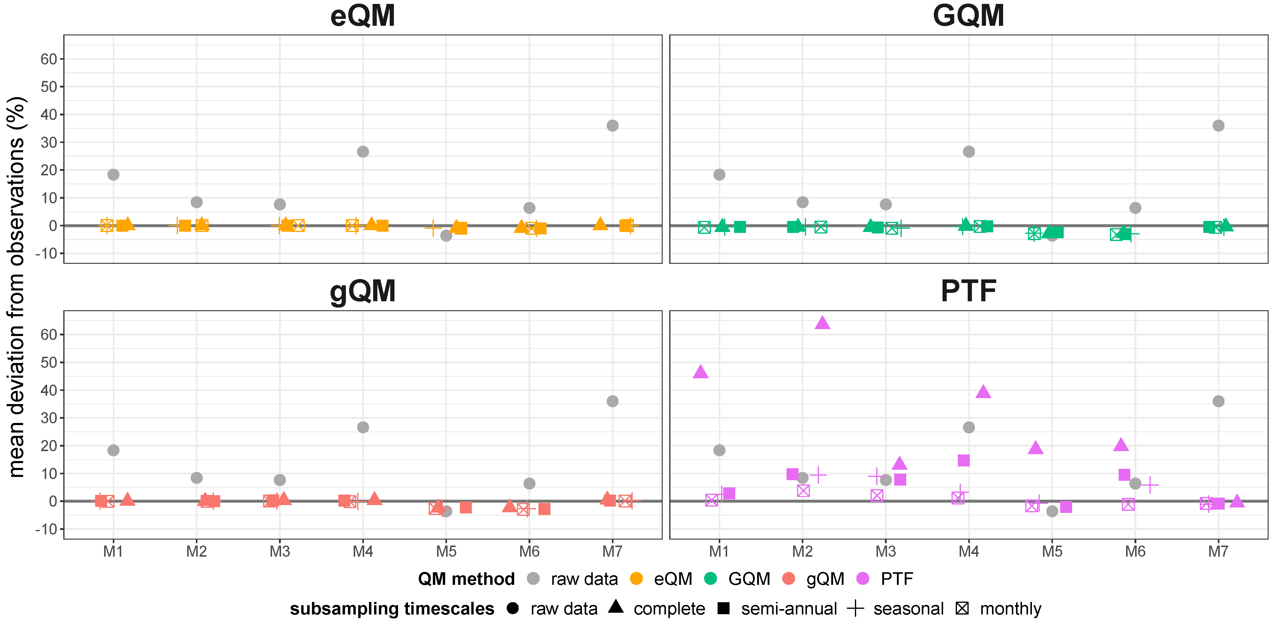
The uncorrected RCM simulations showed considerable deviations from the observations, as Figure 2 shows exemplary for the mean annual precipitation sum. Six out of the seven uncorrected RCM simulations overestimated the mean annual precipitation sum between approximately 5% and up to 35%. One RCM simulation (M5) underestimated it by approximately 5%. The majority of the applied BCs resulted in very good corrections of this characteristic. Only the QM method PTF failed in several cases to correct the bias for the coarser subsampling timescales (especially complete, but also semi-annual), even increasing it to deviations of up to 65% in one case. The QM method eQM resulted in the best corrections based on this characteristic.
The analysis of the annual cycle also showed substantial deviations from the observations for the uncorrected RCM simulations, ranging between approximately 5% and 15% (Figure 3). The bias-corrected data showed no clear improvement when no subsampling was applied in the BC (complete). With subsampling, the match of the annual cycle between the bias-corrected climate projections and observations improved. The finer the subsampling timescale, the better the match. The best match was again obtained when applying the eQM method. For climate projection M5, the very large deviation in the annual cycle of the uncorrected climate projections could be corrected to a nearly perfect fit by all QM methods when applying the monthly subsampling. For climate projection M2, the QM method PTF failed to improve the match of the annual cycle with the observations regardless of the subsampling timescale used.

3.2. Climate Change Signals

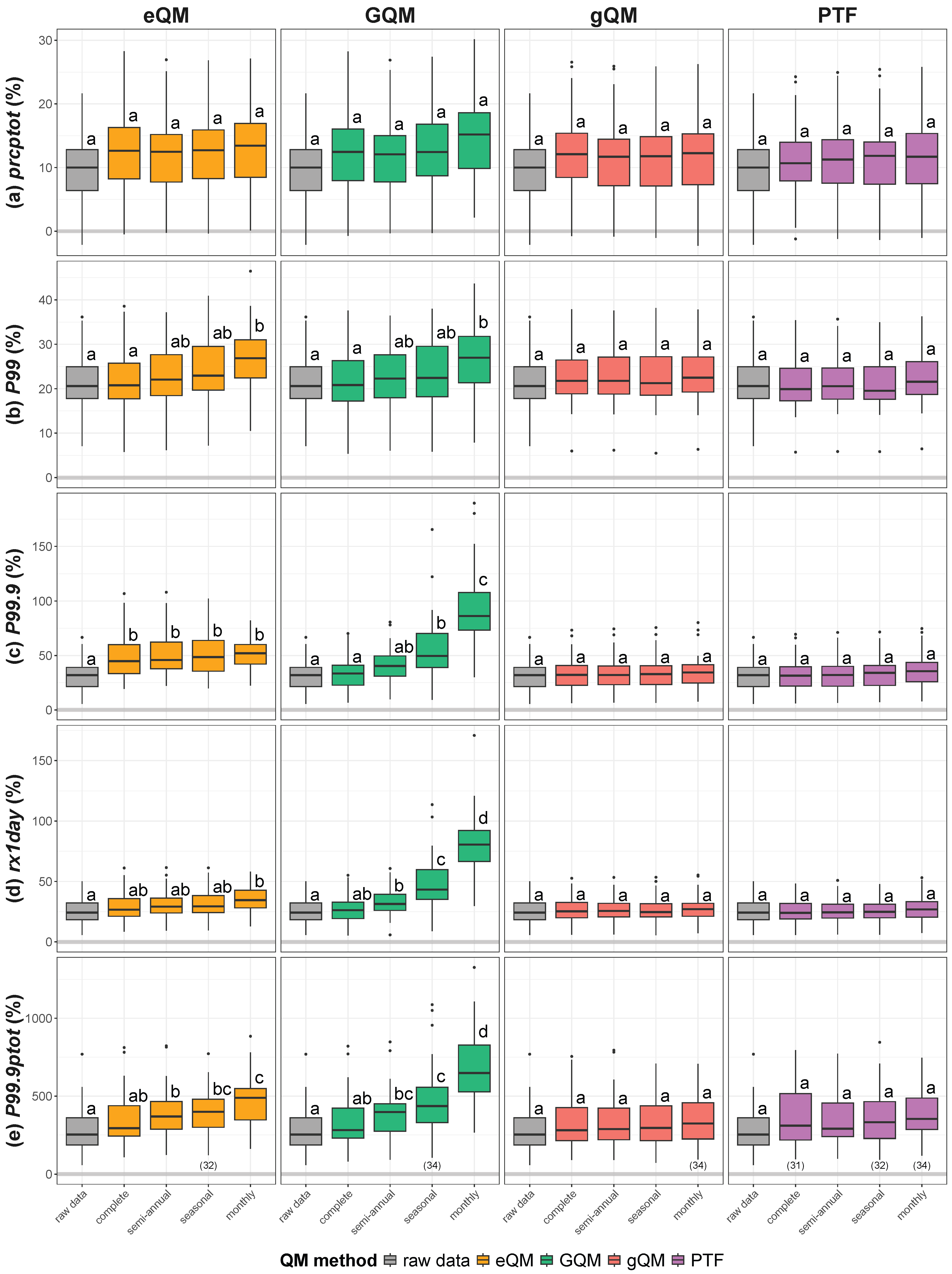
Figure 4 shows the CCSs for the period 2071 to 2100 compared to the base period 1971 to 2000 for the the five indices used in this study. BC did not significantly change the CCSs for the mean annual precipitation sum for wet days (prcptot) regardless of the QM method or subsampling timescale used (Figure 4a).
However, we observed that the BC affected the CCSs for the other indices, dependending on the QM method and the subsampling timescale. The CCSs of index P 99 increased when applying the more complex QM methods eQM and GQM with the monthly subsampling (Figure 4b). For P 99.9 , the CCSs generally increased when the climate projections were bias corrected with eQM. However, there were no further differences in the CCSs between the different subsampling timescales for this QM method (Figure 4c). For GQM, the CCSs of the seasonally bias-corrected climate projections were larger than those of the uncorrected climate projections as well as those of the bias-corrected climate projections without subsampling (complete). In addition, the CCSs for the monthly GQM were even larger than those of the seasonally corrected climate projections. For index rx1day, the CCSs of the climate projections using eQM increased only for the monthly subsampling timescale (Figure 4d). For GQM, however, the CCSs already increased with a semi-annual subsampling compared to the CCSs of the uncorrected climate projections. The CCSs of rx1day then increased again with seasonal respectively monthly subsampling for GQM. Figure 4e shows that the results for index P 99.9 ptot are comparable to those for index rx1day when using the QM method GQM. When applying the QM method eQM, the CCSs increased with a semi-annual subsampling timescale compared to the uncorrected climate projections, and the CCSs of the climate projections increased again with a monthly subsampling timescale. For all five indices, no increase of the CCSs was observed when applying the less complex QM methods gQM and PTF for the BC regardless of the subsampling timescale used.

4. Discussion

The analysis showed that all QM methods generally resulted in good corrections of the RCM simulations in relation to observations. Overall, eQM showed the best corrections for the data of the calibration period. This was to be expected due to its empirical nature and is in agreement with other studies [13,24,39,55,56,57]. For QM method PTF, deficiencies were found in individual cases when applied without or with semi-annual subsampling. Instead of reducing the deviation from the observations, the rsm values increased. This is due to failed calibrations of the BC transfer function at single grid cells, resulting in much too high corrected values for the tail of the distribution. As a result, these were reflected in the mean annual precipitation sum and hence also in the rsm values.
All QM methods were predominantly able to correct for errors in the annual cycle when applied with subsampling. The correction was again best for the QM method eQM. The results also clearly showed that the finer the subsampling timescale, the better the correction of the annual cycle.
However, the results for the effect of applying subsampling in the BC on the CCS have shown that there are also significant negative impacts. For several indices, we observed changes in the CCS when applying subsampling in the BC for the more complex QM methods eQM and GQM. Potentially, these changes of the CCS could be a positive effect, e.g., if there were incorrect representations of processes or for example the annual cycle. This is one of the main reasons why subsampling is applied in the BC process [36,37,38,39]. However, we explicitly used indices in this study that are independent of the annual cycle. On the contrary, it is obvious that these changes in the CCS are not a positive consequence of the subsampling. First, this is because we did not observe such changes for the less complex QM methods when these were applied with subsampling. Second, studies have shown that the robustness of the BC decreases when reducing the calibration sample size. Reiter et al. [38,46] analysed the effects of a reduction of the length of the calibration period and the effects of a decreasing calibration sample size due to subsampling on the QM performance and robustness in detail. Their results showed a decrease in BC performance and robustness for certain QM methods. Other studies have consistently shown that reducing the calibration sample size leads to an increase in sampling uncertainty [36,37,40,41,42]. Additionally, the more complex QM methods are vulnerable to overfitting [38,43,44,46]. The observed changes in the CCS for eQM and GQM are clearly connected to these issues. This shows on the grid cell level, where very high and implausible values appear at single grid cells, which are ultimately responsible for the change of the CCS. Such implausible bias-corrected values can have disastrous consequences in climate change impact studies. Studies in the important field of extreme value analysis (e.g., [58,59,60]) focus on the tail of the distribution, and therefore implausibly high values can lead to incorrect results and ultimately to incorrect decisions in climate change adaptation.

5. Conclusions

The application of a BC using any of the four QM methods without subsampling did not significantly affect the CCS of any index except in one case. The results showed a clear advantage of applying subsampling in the BC on the agreement of the annual cycle between the RCM simulations and the observations. However, the results also showed that not all subsampling timescales are safe to use for all QM methods. For the less complex QM methods gQM and PTF, we did not observe any significant changes in the CCS even when applying the monthly subsampling. This is consistent with studies on their BC robustness [38,46]. For eQM, at most the seasonal subsampling is to be recommended, which is also consistent with other studies [38,46] and also with more general studies of BC performance [36,37]. The QM method GQM was found to be even more vulnerable, and here even semi-annual subsampling changed the CCS for some indices, which is more extreme than the findings in the studies of their BC robustness [38,46] where at least a semi-annual subsampling could be recommended. When applying BC with subsampling, we would recommend to also apply a BC without subsampling in order to be able to assess the effect of the subsampling on the CCS.

Author Contributions

Conceptualisation, P.R. and M.C.C.; methodology, P.R.; software, P.R.; validation, P.R.; formal analysis, P.R.; investigation, P.R.; resources, P.R.; data curation, P.R.; writing—original draft preparation, P.R. and M.C.C.; writing—review and editing, P.R. and M.C.C.; visualisation, P.R.; supervision, M.C.C.; project administration, P.R. All authors have read and agreed to the published version of the manuscript.

Funding

This research received no external funding.

Data Availability Statement

The original data presented in the study are openly available in FigShare at https://doi.org/10.6084/m9.figshare.26502622.

Acknowledgments

We acknowledge the World Climate Research Programme’s Working Group on Regional Climate, and the Working Group on Coupled Modelling, former coordinating body of CORDEX and responsible panel for CMIP5. We also thank the climate modelling groups (listed in Table 1 of this paper) for producing and making available their model output. We also acknowledge the Earth System Grid Federation infrastructure, which is an international effort led by the U.S. Department of Energy’s Program for Climate Model Diagnosis and Intercomparison, the European Network for Earth System Modelling and other partners in the Global Organisation for Earth System Science Portals (GO-ESSP).

Conflicts of Interest

The authors declare no conflicts of interest.

Abbreviations

The following abbreviations are used in this manuscript:
rsmrobust spatial mean
QMquantile mapping
BCbias correction
CCSclimate change signal
RCMregional climate model
GCMglobal climate model

References

  1. Intergovernmental Panel On Climate Change (IPCC). Climate Change 2021—The Physical Science Basis: Working Group I Contribution to the Sixth Assessment Report of the Intergovernmental Panel on Climate Change, 1st ed.; Cambridge University Press: Cambridge, UK, 2023. [Google Scholar] [CrossRef]
  2. Haerter, J.O.; Hagemann, S.; Moseley, C.; Piani, C. Climate model bias correction and the role of timescales. Hydrol. Earth Syst. Sci. 2011, 15, 1065–1079. [Google Scholar] [CrossRef]
  3. Ehret, U.; Zehe, E.; Wulfmeyer, V.; Warrach-Sagi, K.; Liebert, J. HESS Opinions “Should we apply bias correction to global and regional climate model data?”. Hydrol. Earth Syst. Sci. 2012, 16, 3391–3404. [Google Scholar] [CrossRef]
  4. Vogel, E.; Johnson, F.; Marshall, L.; Bende-Michl, U.; Wilson, L.; Peter, J.R.; Wasko, C.; Srikanthan, S.; Sharples, W.; Dowdy, A.; et al. An evaluation framework for downscaling and bias correction in climate change impact studies. J. Hydrol. 2023, 622, 129693. [Google Scholar] [CrossRef]
  5. Papadimitriou, L.V.; Koutroulis, A.G.; Grillakis, M.G.; Tsanis, I.K. High-end climate change impact on European runoff and low flows—exploring the effects of forcing biases. Hydrol. Earth Syst. Sci. 2016, 20, 1785–1808. [Google Scholar] [CrossRef]
  6. Trancoso, R.; Syktus, J.; Toombs, N.; Ahrens, D.; Wong, K.K.H.; Pozza, R.D. Heatwaves intensification in Australia: A consistent trajectory across past, present and future. Sci. Total Environ. 2020, 742, 140521. [Google Scholar] [CrossRef] [PubMed]
  7. Eccles, R.; Zhang, H.; Hamilton, D.; Trancoso, R.; Syktus, J. Impacts of climate change on streamflow and floodplain inundation in a coastal subtropical catchment. Adv. Water Resour. 2021, 147, 103825. [Google Scholar] [CrossRef]
  8. Maraun, D.; Wetterhall, F.; Ireson, A.M.; Chandler, R.E.; Kendon, E.J.; Widmann, M.; Brienen, S.; Rust, H.W.; Sauter, T.; Themeßl, M.; et al. Precipitation downscaling under climate change: Recent developments to bridge the gap between dynamical models and the end user. Rev. Geophys. 2010, 48, RG3003. [Google Scholar] [CrossRef]
  9. Maraun, D.; Huth, R.; Gutiérrez, J.M.; Martín, D.S.; Dubrovsky, M.; Fischer, A.; Hertig, E.; Soares, P.M.M.; Bartholy, J.; Pongrácz, R.; et al. The VALUE perfect predictor experiment: Evaluation of temporal variability. Int. J. Climatol. 2019, 39, 3786–3818. [Google Scholar] [CrossRef]
  10. Widmann, M.; Bedia, J.; Gutiérrez, J.M.; Bosshard, T.; Hertig, E.; Maraun, D.; Casado, M.J.; Ramos, P.; Cardoso, R.M.; Soares, P.M.M.; et al. Validation of spatial variability in downscaling results from the VALUE perfect predictor experiment. Int. J. Climatol. 2019, 39, 3819–3845. [Google Scholar] [CrossRef]
  11. Maraun, D. Bias Correction, Quantile Mapping, and Downscaling: Revisiting the Inflation Issue. J. Clim. 2013, 26, 2137–2143. [Google Scholar] [CrossRef]
  12. Wilcke, R.A.I.; Mendlik, T.; Gobiet, A. Multi-variable error correction of regional climate models. Clim. Chang. 2013, 120, 871–887. [Google Scholar] [CrossRef]
  13. Enayati, M.; Bozorg-Haddad, O.; Bazrafshan, J.; Hejabi, S.; Chu, X. Bias correction capabilities of quantile mapping methods for rainfall and temperature variables. J. Water Clim. Chang. 2021, 12, 401–419. [Google Scholar] [CrossRef]
  14. Themeßl, M.J.; Gobiet, A.; Leuprecht, A. Empirical-statistical downscaling and error correction of daily precipitation from regional climate models. Int. J. Climatol. 2011, 31, 1530–1544. [Google Scholar] [CrossRef]
  15. Teutschbein, C.; Seibert, J. Bias correction of regional climate model simulations for hydrological climate-change impact studies: Review and evaluation of different methods. J. Hydrol. 2012, 456–457, 12–29. [Google Scholar] [CrossRef]
  16. Fang, G.H.; Yang, J.; Chen, Y.N.; Zammit, C. Comparing bias correction methods in downscaling meteorological variables for a hydrologic impact study in an arid area in China. Hydrol. Earth Syst. Sci. 2015, 19, 2547–2559. [Google Scholar] [CrossRef]
  17. Hagemann, S.; Chen, C.; Haerter, J.O.; Heinke, J.; Gerten, D.; Piani, C. Impact of a Statistical Bias Correction on the Projected Hydrological Changes Obtained from Three GCMs and Two Hydrology Models. J. Hydrometeor. 2011, 12, 556–578. [Google Scholar] [CrossRef]
  18. Maurer, E.P.; Pierce, D.W. Bias correction can modify climate model simulated precipitation changes without adverse effect on the ensemble mean. Hydrol. Earth Syst. Sci. 2014, 18, 915–925. [Google Scholar] [CrossRef]
  19. Wootten, A.M.; Dixon, K.W.; Adams-Smith, D.J.; McPherson, R.A. Statistically downscaled precipitation sensitivity to gridded observation data and downscaling technique. Int. J. Climatol. 2021, 41, 980–1001. [Google Scholar] [CrossRef]
  20. Zhang, H.; Chapman, S.; Trancoso, R.; Toombs, N.; Syktus, J. Assessing the impact of bias correction approaches on climate extremes and the climate change signal. Meteorol. Appl. 2024, 31, e2204. [Google Scholar] [CrossRef]
  21. Gobiet, A.; Suklitsch, M.; Heinrich, G. The effect of empirical-statistical correction of intensity-dependent model errors on the temperature climate change signal. Hydrol. Earth Syst. Sci. 2015, 19, 4055–4066. [Google Scholar] [CrossRef]
  22. Boberg, F.; Christensen, J.H. Overestimation of Mediterranean summer temperature projections due to model deficiencies. Nat. Clim. Chang. 2012, 2, 433–436. [Google Scholar] [CrossRef]
  23. Ivanov, M.A.; Luterbacher, J.; Kotlarski, S. Climate Model Biases and Modification of the Climate Change Signal by Intensity-Dependent Bias Correction. J. Clim. 2018, 31, 6591–6610. [Google Scholar] [CrossRef]
  24. Cannon, A.J.; Sobie, S.R.; Murdock, T.Q. Bias Correction of GCM Precipitation by Quantile Mapping: How Well Do Methods Preserve Changes in Quantiles and Extremes? J. Clim. 2015, 28, 6938–6959. [Google Scholar] [CrossRef]
  25. Pierce, D.W.; Cayan, D.R.; Maurer, E.P.; Abatzoglou, J.T.; Hegewisch, K.C. Improved Bias Correction Techniques for Hydrological Simulations of Climate Change*. J. Hydrometeorol. 2015, 16, 2421–2442. [Google Scholar] [CrossRef]
  26. Tefera, G.W.; Dile, Y.T.; Ray, R.L. Evaluating the Impact of Statistical Bias Correction on Climate Change Signal and Extreme Indices in the Jemma Sub-Basin of Blue Nile Basin. Sustainability 2023, 15, 10513. [Google Scholar] [CrossRef]
  27. Casanueva, A.; Herrera, S.; Iturbide, M.; Lange, S.; Jury, M.; Dosio, A.; Maraun, D.; Gutiérrez, J.M. Testing bias adjustment methods for regional climate change applications under observational uncertainty and resolution mismatch. Atmos. Sci. Lett. 2020, 21, e978. [Google Scholar] [CrossRef]
  28. Hempel, S.; Frieler, K.; Warszawski, L.; Schewe, J.; Piontek, F. A trend-preserving bias correction – the ISI-MIP approach. Earth Syst. Dynam. 2013, 4, 219–236. [Google Scholar] [CrossRef]
  29. Grillakis, M.G.; Koutroulis, A.G.; Daliakopoulos, I.N.; Tsanis, I.K. A method to preserve trends in quantile mapping bias correction of climate modeled temperature. Earth Syst. Dynam. 2017, 8, 889–900. [Google Scholar] [CrossRef]
  30. Switanek, M.B.; Troch, P.A.; Castro, C.L.; Leuprecht, A.; Chang, H.I.; Mukherjee, R.; Demaria, E.M.C. Scaled distribution mapping: A bias correction method that preserves raw climate model projected changes. Hydrol. Earth Syst. Sci. 2017, 21, 2649–2666. [Google Scholar] [CrossRef]
  31. Maraun, D.; Shepherd, T.G.; Widmann, M.; Zappa, G.; Walton, D.; Gutiérrez, J.M.; Hagemann, S.; Richter, I.; Soares, P.M.M.; Hall, A.; et al. Towards process-informed bias correction of climate change simulations. Nat. Clim. Chang. 2017, 7, 764–773. [Google Scholar] [CrossRef]
  32. Maraun, D. Bias Correcting Climate Change Simulations - a Critical Review. Curr. Clim. Chang. Rep. 2016, 2, 211–220. [Google Scholar] [CrossRef]
  33. Maraun, D.; Truhetz, H.; Schaffer, A. Regional Climate Model Biases, Their Dependence on Synoptic Circulation Biases and the Potential for Bias Adjustment: A Process-Oriented Evaluation of the Austrian Regional Climate Projections. Geophys. Res. Atmos. 2021, 126, e2020JD032824. [Google Scholar] [CrossRef]
  34. Dosio, A. Projections of climate change indices of temperature and precipitation from an ensemble of bias-adjusted high-resolution EURO-CORDEX regional climate models. Geophys. Res. Atmos. 2016, 121, 5488–5511. [Google Scholar] [CrossRef]
  35. Ugolotti, A.; Anders, T.; Lanssens, B.; Hickler, T.; François, L.; Tölle, M.H. Impact of bias correction on climate change signals over central Europe and the Iberian Peninsula. Front. Environ. Sci. 2023, 11, 1116429. [Google Scholar] [CrossRef]
  36. Räty, O.; Räisänen, J.; Ylhäisi, J.S. Evaluation of delta change and bias correction methods for future daily precipitation: Intermodel cross-validation using ENSEMBLES simulations. Clim. Dyn. 2014, 42, 2287–2303. [Google Scholar] [CrossRef]
  37. Rajczak, J.; Kotlarski, S.; Salzmann, N.; Schär, C. Robust climate scenarios for sites with sparse observations: A two-step bias correction approach. Int. J. Climatol. 2016, 36, 1226–1243. [Google Scholar] [CrossRef]
  38. Reiter, P.; Gutjahr, O.; Schefczyk, L.; Heinemann, G.; Casper, M. Does applying quantile mapping to subsamples improve the bias correction of daily precipitation? Int. J. Climatol. 2018, 38, 1623–1633. [Google Scholar] [CrossRef]
  39. Gutiérrez, J.M.; Maraun, D.; Widmann, M.; Huth, R.; Hertig, E.; Benestad, R.; Roessler, O.; Wibig, J.; Wilcke, R.; Kotlarski, S.; et al. An intercomparison of a large ensemble of statistical downscaling methods over Europe: Results from the VALUE perfect predictor cross-validation experiment. Int. J. Climatol. 2019, 39, 3750–3785. [Google Scholar] [CrossRef]
  40. Boé, J.; Terray, L.; Habets, F.; Martin, E. Statistical and dynamical downscaling of the Seine basin climate for hydro-meteorological studies. Int. J. Climatol. 2007, 27, 1643–1655. [Google Scholar] [CrossRef]
  41. Berg, P.; Feldmann, H.; Panitz, H.J. Bias correction of high resolution regional climate model data. J. Hydrol. 2012, 448–449, 80–92. [Google Scholar] [CrossRef]
  42. Räisänen, J.; Räty, O. Projections of daily mean temperature variability in the future: Cross-validation tests with ENSEMBLES regional climate simulations. Clim. Dyn. 2013, 41, 1553–1568. [Google Scholar] [CrossRef]
  43. Piani, C.; Weedon, G.P.; Best, M.; Gomes, S.M.; Viterbo, P.; Hagemann, S.; Haerter, J.O. Statistical bias correction of global simulated daily precipitation and temperature for the application of hydrological models. J. Hydrol. 2010, 395, 199–215. [Google Scholar] [CrossRef]
  44. Gudmundsson, L.; Bremnes, J.B.; Haugen, J.E.; Engen-Skaugen, T. Technical Note: Downscaling RCM precipitation to the station scale using statistical transformations—A comparison of methods. Hydrol. Earth Syst. Sci. 2012, 16, 3383–3390. [Google Scholar] [CrossRef]
  45. Piani, C.; Haerter, J.O. Two dimensional bias correction of temperature and precipitation copulas in climate models. Geophys. Res. Lett. 2012, 39, L20401. [Google Scholar] [CrossRef]
  46. Reiter, P.; Gutjahr, O.; Schefczyk, L.; Heinemann, G.; Casper, M. Bias correction of ENSEMBLES precipitation data with focus on the effect of the length of the calibration period. Meteorol. Z. 2016, 25, 85–96. [Google Scholar] [CrossRef]
  47. Jacob, D.; Petersen, J.; Eggert, B.; Alias, A.; Christensen, O.B.; Bouwer, L.M.; Braun, A.; Colette, A.; Déqué, M.; Georgievski, G.; et al. EURO-CORDEX: New high-resolution climate change projections for European impact research. Reg. Environ. Chang. 2014, 14, 563–578. [Google Scholar] [CrossRef]
  48. Rauthe, M.; Steiner, H.; Riediger, U.; Mazurkiewicz, A.; Gratzki, A. A Central European precipitation climatology? Part I: Generation and validation of a high-resolution gridded daily data set (HYRAS). Meteorol. Z. 2013, 22, 235–256. [Google Scholar] [CrossRef]
  49. Piani, C.; Haerter, J.O.; Coppola, E. Statistical bias correction for daily precipitation in regional climate models over Europe. Theor. Appl. Climatol. 2010, 99, 187–192. [Google Scholar] [CrossRef]
  50. Gutjahr, O.; Heinemann, G. Comparing precipitation bias correction methods for high-resolution regional climate simulations using COSMO-CLM. Theor. Appl. Climatol. 2013, 114, 511–529. [Google Scholar] [CrossRef]
  51. Denis, B.; Laprise, R.; Caya, D.; Côté, J. Downscaling ability of one-way nested regional climate models: The Big-Brother Experiment. Clim. Dyn. 2002, 18, 627–646. [Google Scholar] [CrossRef]
  52. Boberg, F.; Berg, P.; Thejll, P.; Gutowski, W.J.; Christensen, J.H. Improved confidence in climate change projections of precipitation evaluated using daily statistics from the PRUDENCE ensemble. Clim. Dyn. 2008, 32, 1097–1106. [Google Scholar] [CrossRef]
  53. Zwiers, F.W.; Zhang, X. Guidelines on Analysis of Extremes in a Changing Climate in Support of Informed Decisions for Adaptation; Technical Report 72; World Meteorological Organization (WMO): Geneva, Switzerland, 2009. [Google Scholar]
  54. Wilcoxon, F. Individual Comparisons by Ranking Methods. Biom. Bull. 1945, 1, 80–83. [Google Scholar] [CrossRef]
  55. Themeßl, M.J.; Gobiet, A.; Heinrich, G. Empirical-statistical downscaling and error correction of regional climate models and its impact on the climate change signal. Clim. Chang. 2012, 112, 449–468. [Google Scholar] [CrossRef]
  56. Lafon, T.; Dadson, S.; Buys, G.; Prudhomme, C. Bias correction of daily precipitation simulated by a regional climate model: A comparison of methods. Int. J. Climatol. 2013, 33, 1367–1381. [Google Scholar] [CrossRef]
  57. Luo, M.; Liu, T.; Meng, F.; Duan, Y.; Frankl, A.; Bao, A.; De Maeyer, P. Comparing Bias Correction Methods Used in Downscaling Precipitation and Temperature from Regional Climate Models: A Case Study from the Kaidu River Basin in Western China. Water 2018, 10, 1046. [Google Scholar] [CrossRef]
  58. De Luca, D.L.; Ridolfi, E.; Russo, F.; Moccia, B.; Napolitano, F. Climate change effects on rainfall extreme value distribution: The role of skewness. J. Hydrol. 2024, 634, 130958. [Google Scholar] [CrossRef]
  59. Kotz, M.; Lange, S.; Wenz, L.; Levermann, A. Constraining the Pattern and Magnitude of Projected Extreme Precipitation Change in a Multimodel Ensemble. J. Clim. 2024, 37, 97–111. [Google Scholar] [CrossRef]
  60. Pant, M.; Bhatla, R.; Ghosh, S.; Das, S.; Mall, R.K. How climate change is affecting the summer monsoon extreme rainfall pattern over the Indo-Gangetic Plains of India: Present and future perspectives. Clim. Dyn. 2024, 62, 1055–1075. [Google Scholar] [CrossRef]
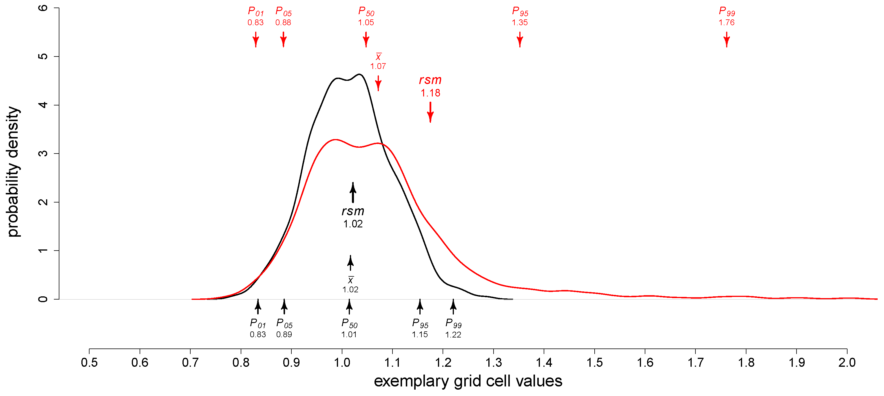
Figure 1. Visualisation of the rsm value for two exemplary distributions. Additionally, the arithmetic mean x ¯ and the percentiles used to calculate rsm ( P 01 , P 05 , the median P 50 , P 95 and P 99 ) are shown.
Hydrology 11 00143 g001
Figure 2. rsm values for the deviation of the mean annual precipitation sum for the uncorrected and bias-corrected climate projections from the observations for the base period 1951 to 2005.
Hydrology 11 00143 g002
Figure 3. rsm values of the match of the monthly assessed annual cycle between observations and the uncorrected as well as bias-corrected RCM simulations for the base period 1951 to 2005.
Hydrology 11 00143 g003
Figure 4. rsm values of the CCSs for the period 2071 to 2100 compared to the base period 1971 to 2000 for indices (a) prcptot, (b) P 99 , (c) P 99.9 , (d) rx1day and (e) P 99.9 ptot depending on the QM method used. Significant differences ( α = 0.05) are indicated by the letters. Each boxplot is based on 35 rsm values (7 climate projections × 5 20% samples) unless otherwise noted below the respective boxplot. Lower numbers for some boxplots are due to infinite values at single grid cells.
Hydrology 11 00143 g004
Table 1. Climate projections from the CORDEX project used in this study.
GCM 1RunRCM 2Institution
M1CNRM-CERFACS-CNRM-CM5r1i1p1CLMcom-CCLM4-8-17Climate Limited-area Modelling Community
M2ICHEC-EC-EARTHr12i1p1CLMcom-CCLM4-8-17Climate Limited-area Modelling Community
M3ICHEC-EC-EARTHr1i1p1KNMI-RACMO22ERoyal Netherlands Meteorological Institute
M4ICHEC-EC-EARTHr3i1p1DMI-HIRHAM5Danish Meteorological Institute
M5MOHC-HadGEM2-ESr1i1p1CLMcom-CCLM4-8-17Climate Limited-area Modelling Community
M6MOHC-HadGEM2-ESr1i1p1KNMI-RACMO22ERoyal Netherlands Meteorological Institute
M7MPI-M-MPI-ESM-LRr1i1p1CLMcom-CCLM4-8-17Climate Limited-area Modelling Community
1 Global Climate Model. 2 Regional Climate Model.
Table 2. QM methods used in this study.
QM MethodTypeDescriptionReference
eQMnon-parametricempirical QMBoé et al. [40]
gQMparametricgamma distribution based QMPiani et al. [49]
GQMparametricgamma distribution and GPD based QMGutjahr and Heinemann [50]
PTFsemi-parametricexponential tendency toward an asymptotePiani et al. [43]
Table 3. Subsampling timescales used in his study.
Subsampling TimescaleReferred to asNumber of Subsamples
no subsamplingcomplete1
separately for winter (NDJFMA) and summer (MJJASO)semi-annual2
separately for each meteorological seasonseasonal4
separately for each calendar monthmonthly12
Table 4. Indices used in this study to assess the effect of BC on the CCS.
IndexDescriptionReference
prcptotmean annual precipitation sum for wet-days (≥1 mm)Zwiers and Zhang [53]
P 99 99th percentile of precipitation on wet days (≥1 mm)-
P 99.9 99.9th percentile of precipitation on wet days (≥1 mm)-
rx1daymean annual maximum daily precipitationZwiers and Zhang [53]
P 99.9 ptotprecipitation amount for days with precipitation larger than the 99.9th percentile on wet days (≥1 mm) of the base period 1951 to 2005modified in reference to Zwiers and Zhang [53]
Disclaimer/Publisher’s Note: The statements, opinions and data contained in all publications are solely those of the individual author(s) and contributor(s) and not of MDPI and/or the editor(s). MDPI and/or the editor(s) disclaim responsibility for any injury to people or property resulting from any ideas, methods, instructions or products referred to in the content.