Article

Simulating the Potential Evapotranspiration of Egypt Using the RegCM4: Sensitivity to the Land Surface and Boundary Layer Parameterizations

by
Samy A. Anwar
1,* and
Christiana F. Olusegun
2
1
Egyptian Meteorological Authority, Qobry EL-Kobba, Cairo P.O. Box 11784, Egypt
2
Department of Earth and Environmental Sciences, Michigan State University, East Lansing, MI 48824, USA
*
Author to whom correspondence should be addressed.
Hydrology 2024, 11(8), 121; https://doi.org/10.3390/hydrology11080121
Submission received: 7 July 2024 / Revised: 12 August 2024 / Accepted: 13 August 2024 / Published: 15 August 2024
(This article belongs to the Section Hydrology–Climate Interactions)

Abstract

:
Assessing the daily water requirements of crops and understanding the severity of drought necessitates precise estimation of potential evapotranspiration (PET), particularly in regions with arid climates such as Egypt. In the present study, the RegCM4 regional climate model was used to investigate the sensitivity of the PET of Egypt to two land surface schemes and boundary layer parameterizations. The land surface schemes are the Biosphere Atmosphere Transfer System (BATS) and the Community Land Model version 4.5 (CLM45). The boundary layer schemes considered are the HOLTSLAG (HOLT) and University of Washington (UW). To accomplish this task, four 32-year simulations were conducted spanning from 1979 to 2010, with the first two years considered as spin up. The ERA-Interim reanalysis was used to downscale the RegCM4 model. The simulated PET was evaluated with respect to the high-resolution ERA5-land PET-based product (hPET). The results showed that the BATS showed a bias of −0.8 to −1.8 mm day−1, while the CLM45 showed a bias of −0.8 to −3 mm day−1. Also, fine-tuning the coefficient of the daily mean air temperature succeeded in reducing the PET bias. Additionally, the UW had a lower PET bias than that noted in HOLT. To further reduce the PET bias, the linear-scaling (LS) bias-correction method was used. The LS showed its potential skills in reducing the mean bias of the PET from −2.2 to +0.4 mm day−1 in the evaluation period and to ±0.2 mm day−1 in the validation period. Furthermore, the added value of the LS was confirmed concerning the climatological annual cycle in different locations representing different climate zones of Egypt. In conclusion, accurate estimation of the PET can be ensured using the BATS, the UW schemes, and the LS technique in the present climate or under different warming scenarios.

1. Introduction

Evapotranspiration (ET) is an important variable in the global/regional terrestrial water cycle. ET plays a vital role in controlling the agricultural production, irrigation rate, environmental balance, and ecosystem stability [1,2,3,4]. Also, ET is affected by the accelerated rate of climate change as a global challenge in the 21st century [5,6]. There are multiple definitions to express the ET changes such as potential evapotranspiration (PET), reference evapotranspiration (ETo), crop evapotranspiration, and actual evapotranspiration [2]. PET is defined as the maximum rate of ET given the meteorological condition unlimited supply of water. It is important to highlight that ETo and PET share the same concept, except for that ETo is assigned to a healthy grass of height 0.12 m, a fixed surface resistance of 70 s m−1, and an albedo of 0.23.
The Food and Agriculture Organization (FAO) recommends the Penman–Monteith (PM [2]) equation to estimate the PET/ETo because it considers the physical exchange of water and energy fluxes between the surface and atmosphere. Nonetheless, the PM method does exhibit certain constraints, including (1) the requirement for numerous meteorological inputs, which may not always be readily available in all locations or at all times and (2) the reliance on empirical calculations for most variables, which introduces a degree of uncertainty into the estimated reference evapotranspiration (ETo) [7]. The authors of [8,9] stated that the PM is not suitable to calculate the PET under conditions of unlimited supply of moisture and very dry conditions. Therefore, there was an urgent need to seek a simple empirical formula that can estimate the PET within the accuracy degree of the PM [10]. The PET empirical formula can be categorized as a temperature-based formula (e.g., [11,12]; HS), radiation-based method (e.g., the Priestley–Taylor method [13]), and mass-transfer-based method [14].
The HS has proven its efficiency in estimating the PET in various regions across the globe. For instance, the authors of [15] investigated the ability of the HS method to calculate daily the daily ETo in the northwest of Iran. Also, the authors of [10] reported that the HS is the suitable alternative method to compute for all climate zones in Iran. Additionally, the authors of [16] reported that the HS can give PET records like the one calculated by the PM. In eastern India, the authors of [17] computed the ETo using the PM method, lysimeter data, and the Variable Infiltration Capacity (VIC-3L) land surface model. Also, they highlighted the added value of using the genetic-algorithm-based bias correction approach [18] to reduce the ETo bias, which increases the efficiency of the HS method with Nash–Sutcliffe efficiency from 30.12 to 81.75%. Because the HS method only requires extraterrestrial solar radiation as well as daily maximum, minimum, and mean air temperature, the HS can be used to track future PET changes (as a function of the temperature) or to make a daily prediction of the PET [19]. Additionally, the HS has been used in various applications such as the investigation of a wide range of hydro-climatic conditions [20], drought assessment, and hydrological modeling [9,17].
Various regional climate models (RCMs) have been used to estimate the PET/ETo under different future warming scenarios. For instance, the authors of [21] used different RCMs and their ensemble average to estimate the ETo over Spain. They showed that the fine tuning of the radiation coefficient can improve the calculated ETo with respect to observations of the PM. Furthermore, they highlighted the added value of considering the ensemble average to reduce the uncertainty of the meteorological inputs involved in the HS. Within the framework of the RegCM4 regional climate model [22], the PET of Egypt has been manipulated for various purposes. For instance, the authors of [23] used the RegCM4 to estimate water loss under the RCP4.5 scenario. Additionally, the authors of [24] examined the sensitivity of the PET to different lateral boundary conditions and checked whether the calibrated HS equation can reduce the PET bias (relative to the original version) compared to the ERA5-land PET-based product.
In Egypt, the authors of [25] investigated the sensitivity of the PET to different options of dynamical downscaling and boundary layer schemes. They observed that the PET is not sensitive to any of the aforementioned options, suggesting that the global incident solar radiation controls the PET changes. It is important to highlight that the HS equation has two versions. The first version is based on the extraterrestrial solar radiation as well as the daily maximum, minimum, and mean air temperature [11], and the second version includes the daily mean air temperature and global incident solar radiation [12]. The authors of [23] exclusively used the temperature-only formula, whereas other studies mentioned have applied the temperature-radiation formula. However, using the temperature-radiation-based formula limits the exploration of the PET’s sensitivity to various physical schemes, as global incident solar radiation remains unaffected by the choice of physical scheme [25]. Hence, to assess the impact of various physical schemes on the PET, this study employed the temperature-only-based formula. This approach necessitated an initial investigation into how different physical schemes affect daily air temperature, followed by an analysis of their influence on the PET.
The authors of [26] compared between the two boundary layer schemes of the RegCM4 (HOLTSLAG—HOLT [27] and University of Washington—UW [28]) concerning the daily mean air temperature. They found that the UW outperforms the HOLT with respect to the ERA5 [29]. Also, the authors of [30] observed that the community land model version 4.5 (CLM45 [31]) is better than the Biosphere Atmosphere Transfer Scheme (BATS [32]) in terms of simulating the daily maximum and minimum air temperature concerning the ERA5. However, the sensitivity of the PET to the land surface scheme was not considered in this study. In this study, we aimed to
  • Compare between the BATS and CLM45 land surface model (with respect to the high-resolution ERA5-land based product, hPET [33]).
  • Fine-tune the coefficients of the HS equation (using the best land surface scheme) and then compare between the original and calibrated version to check the added value of the fine tuning.
  • Assess the sensitivity of the PET to the boundary layer schemes (HOLT and UW) using the calibrated version of the HS to check which scheme is suitable in simulating the PET in comparison with the hPET.
  • Compare between the two versions of the calibrated HS equation: (1) temperature-only-based formula and (2) temperature-radiation-based formula (to examine which formula is the best to compute the PET).
  • Bias-correct the PET (for each season) using the suitable calibrated HS equation (from point 3) with respect to the hPET.
  • Plot the climatological cycle of the PET (before and after applying the bias-correction method) in the validation period.
The structure of this paper is as follows: Section 2 describes the study area and experiment design; Section 3 shows the results of the study; and Section 4 provides the discussion and conclusion.

2. Materials and Methods

2.1. Study Area

Egypt is a nation characterized by its civilization of more than 5000 years and its unique position among the three continents Asia, Africa, and Europe. According to Köppen climate classification [34], Egypt is classified as a hot desert climate (BWh). Geographically, Egypt is bounded by the Mediterranean Sea from the north and the Red Sea from the east. Also, Egypt has a mild winter season with rain falling along coastal areas and a hot and dry summer season (May to September). The authors of [35,36] reported that Egypt has an average amount of precipitation between 20 and 200 mm year−1. In the inland desert areas, temperature shows a notable variability (particularly during summer) from 7 °C at night to 43 °C during the day. Concerning the wind regime, the dominant wind direction is northwest in the Mediterranean Sea. In summer, average high temperatures can exceed 40 °C. Moreover, the Saint Catherine Mountains play an important role in cooling the nighttime temperature compared to other regions of Egypt. The reader can find additional details about Egypt’s climatic features and geographic description in [37,38,39].
In the PET analysis context, the results show a distinct seasonal pattern. The summer season exhibits the most pronounced PET values, ranging from 6 to 10 mm day−1. This is succeeded by the autumn season with 5 to 8 mm day−1. The spring season follows next, with PET values from 3 to 6 mm day−1. The winter season records the lowest PET values, ranging from 1 to 4 mm day−1. These observations are derived from the 30-year climatology of the ERA5-land-based product (hPET [33]). This study contributes to our understanding of PET and its seasonal variations, providing valuable insights for future research.

2.2. Model Description

The regional climate model (RegCM) of the International Center of Theoretical Physics was used in the present study. In essence, the RegCM was developed at the National Center for Atmospheric Research (NCAR, [40,41]). The RegCM is an open-source model and is used for various applications such as regional process studies, paleoclimate simulations, future climate projections, chemistry–climate interactions and aerosol effects, and biosphere–atmosphere interactions [42]. Also, RegCM passed through a series of developments from RegCM1 [41], RegCM2 [43,44], RegCM3 [45], and RegCM4 [22]. Recently, a new version of the RegCM has been developed and tested (RegCM5 [46]). During the time of the study, a stable version of the RegCM5 was not available. Instead, we used version 4.7 of the RegCM (hereafter, RegCM4). The RegCM4 has two dynamical cores: hydrostatic [43] and non-hydrostatic [47].
For the purpose of our study, the hydrostatic core was employed. Additionally, the RegCM4 includes different options for each component such as radiation (Modified Community Climate Model version 3—CCM3 [48] and Rapid Radiation Transfer Model—RRTM [49]), land surface (e.g., BATS [32] and CLM45 [31]), planetary boundary layer (HOLTSLAG—HOLT [29] and University of Washington—UW [30]), and cumulus convection (e.g., MIT [50]). Additional components and options can be found in [22]. In this study, we used the radiation scheme of RRTM and cumulus convection scheme of Emanuel. A comparison between different schemes of the land surface and planetary boundary layer was conducted (see Section 2.3).

2.3. Experimental Design

In this study, we customized the RegCM4’s domain with 25 km grid spacing, 60 grid points in both zonal and meridional directions to approximately cover the area of 24–38° E and 22–34° N. Caution was taken to ensure that the selected domain is away from the boundaries. The ERA-Interim reanalysis of 1.5 degrees (EIN15 [51]) was used to downscale the RegCM4 model to provide the lateral boundary condition and sea surface temperature. Figure 1 shows the surface elevation of Egypt (in meters) including ten locations following the work of [25]. To investigate the influence of different schemes of the land surface and planetary boundary layer, four simulations were conducted in the period 1 January 1979 to 31 December 2010. The first two years were considered as spin up to allow equilibration of the RegCM4 following the work of [52]. Therefore, the actual analysis started at 1 January 1981 and ended at 31 December 2010.
Land surface parameterization comprises the first two simulations: BATS and CLM45. Concerning the planetary boundary layer, the other simulations were designated as HOLT and UW. Note that all simulations were initialized with the ESACCI global satellite soil moisture product [53,54]. To accomplish the purpose of the present study, the PET was calculated using the temperature-only version of the HS. The HS equation is written as
P E T H S = 0.0023 × R a × ( T m a x T m i n ) 0.5 × ( T m e a n + 17.8 ) ,
where Ra is the extraterrestrial solar radiation (expressed in mm day−1 to match the PET unit [2]). Tmax, Tmin, and Tmean are the daily 2 m maximum, minimum, and mean air temperatures, respectively (°C). PETHS is the potential evapotranspiration (in mm day−1). First, a comparison between BATS and CLM45 was conducted. After selecting the best land surface scheme, fine-tuning the coefficient of the Tmean was performed (this step was performed after conduction of various trails to check which coefficient is suitable to be calibrated to obtain low PET bias). The calibrated HS equation can be written as
P E T H S ( c a l i b r a t e d ) = 0.0023 × R a × ( T m a x T m i n ) 0.5 × ( T m e a n + 20.8 ) ,
where PETHS (calibrated) is the calibrated PET (in mm day−1). Then, a comparison between the boundary layer schemes HOLT and UW was performed using the calibrated version of the HS equation. Upon selecting the best boundary layer scheme, a comparison between two calibrated versions of the HS: temperature-only (Equation (2)) and temperature-radiation based formula ([24]; Equation (3)) was performed. Equation (3) can be written as
P E T H S ( c a l i b r a t e d ) = 0.0105 × R S × ( T m e a n + 17.8 )
where Rs is the global incident solar radiation (expressed in mm day−1 to match the PET unit [2]). In all cases, the derived ERA5-land reanalysis product (hPET [33]) was used to evaluate the RegCM4. To possibly reduce the PET bias (using the best calibrated version of the HS equation), a bias-correction method was applied. The bias-correction methods can be categorized as follows: linear scaling (LS), power transformation (PT), local intensity scaling, distribution mapping (DM), variance scaling, quantile mapping (QM), and delta change [55]. The authors of [56] applied the LS, DM, empirical quantile mapping (EQM), and PT to bias-correct the precipitation. On the other hand, DM, EQM, LS, and variance scaling were used to bias-correct the temperature. In our study, we used the LS [57] based on the recommendations of [36,39].
To examine the potential skills of the LS, the period of 1981–2010 was divided into two equal time segments: 1981–1996 (as the evaluation period) and 1997–2010 (as the validation period) to ensure consistency in the PET bias. First, the PET (of the period 1981–1996) was bias-corrected using the LS by means of the climatological bias (between the hPET and RegCM4 for each season: winter, spring, summer, and autumn). After that, the aforementioned climatological bias was applied to the time segment 1997–2010 (to test the LS method outside the evaluation period). It is important to highlight that performance of the RegCM4 (in the evaluation/validation) period was investigated for each grid point. Note that the RegCM4’s output was available in the NetCDF format. Therefore, we used the Climate Data Operator (CDO; https://code.mpimet.mpg.de/projects/cdo/, accessed on 18 October 2022) to calculate the climatological bias of the evaluation period for each grid point. Also, figures (showing the spatial pattern of the PET) were visualized using NCAR Command Language (NCL; https://www.ncl.ucar.edu/, accessed on 18 October 2022).
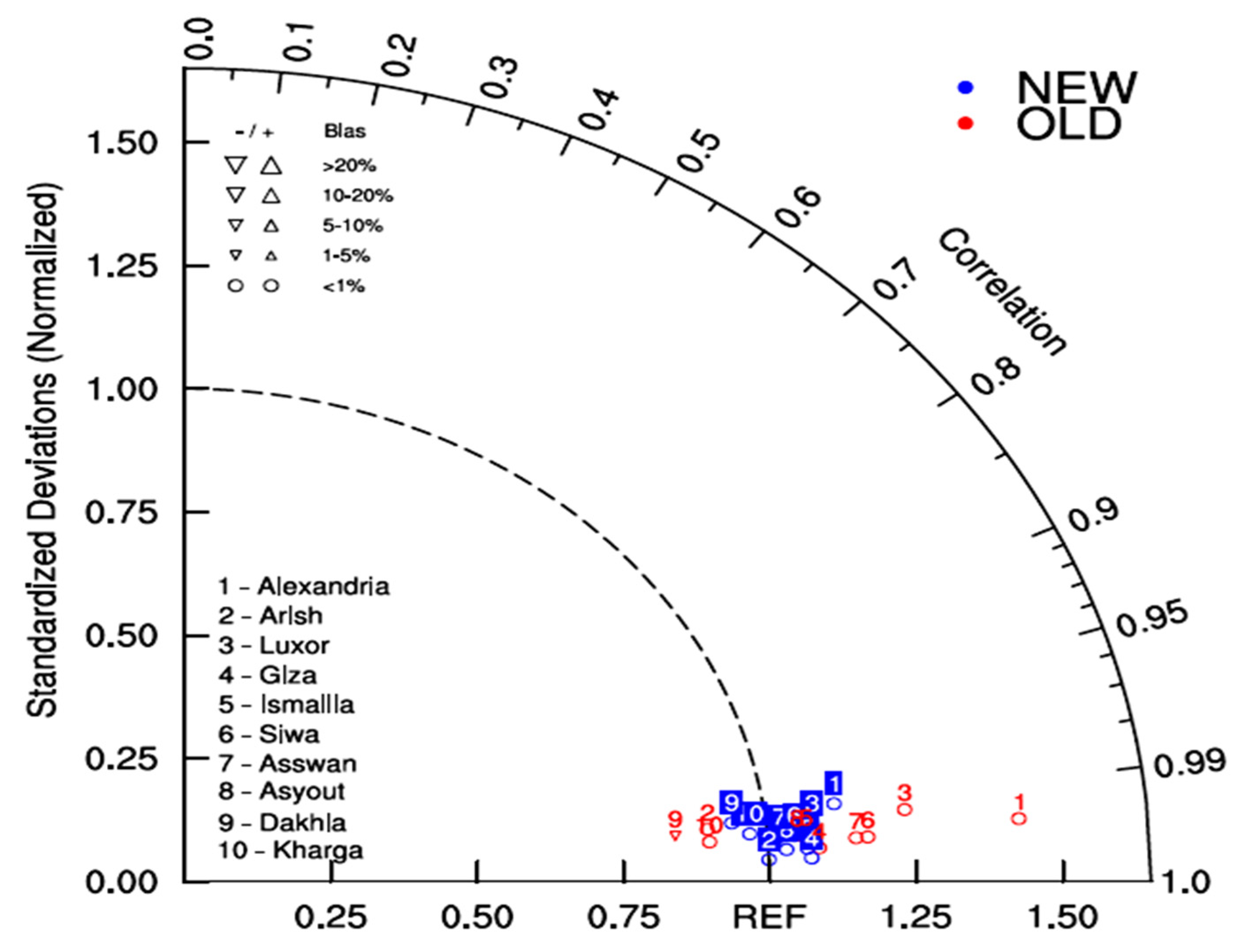
Additionally, performance of the RegCM4 (in the validation period) was quantified using the Taylor diagram [58,59]. The Taylor diagram adopts three statistical metrics to quantify the performance of the reanalysis product or model output with respect to observational dataset: Pearson correlation coefficient (CC), standard deviation ratio (Ratio), and bias percentage (Bias). In this study, we used the Taylor diagram to quantify the RegCM4’s performance (in the validation period) for ten locations (representing different climate zones [25]). The climatological annual cycle (for each location) was extracted (from the RegCM4 output) using netCDF Operator (NCO; https://nco.sourceforge.net/, accessed on 18 October 2022) and bilinear interpolation method [60].

2.4. Observational Dataset

Station data are an important source for monitoring the PET changes on a hierarchy of time scales (ranging from hourly to monthly). However, availability of the long-term observed PET data (for example in Egypt) was a limitation factor to evaluate the RegCM4’s performance. Also, in the present study, it is required to evaluate the PET for each grid point. Therefore, it was necessary to search for alternative products to evaluate the performance of the RegCM4 either spatially or for a specific location. In essence, there are different types of the evapotranspiration products such as MODIS16 (based on the MODerate Resolution Imaging Spectroradiometer MODIS [61]) and Global Land Evaporation Amsterdam Model (GLEAM [62]). However, these products are suitable to compute the PET (for vegetation units only).
Alternatively, a product (not restricted by the land unit) can be suitable for computing the PET such as hPET [33] and Climate Research Unit (CRU [63]). Both hPET and CRU adopt the PM equation to calculate the PET. In essence, the hPET product retrieves the meteorological inputs from the ERA5-land product [64]. Moreover, hPET is available at 0.1 degree grid spacing over the period of 1981 to 2021 over a hierarchy of time scales (hourly, daily sum, and monthly mean/sum). It is important to note that every meteorological input is calculated in the ERA5-land model (available in the period 1950 to 2023). On the other hand, CRU is available in 0.5 degree grid spacing in the period of 1901 to 2022 (only in the monthly mean time scale). Despite of the CRU’s advantage concerning the long time record, it has some limitations, such as (1) wind speed is calculated based on the climatology period of 1961–1990, (2) some derived variables (such as surface net radiation) are calculated using a simple empirical formula based on the total cloud cover, and (3) it is only available in a monthly mean time scale.
As discussed earlier, there are no long-term records of station PET data. Therefore, it was difficult to evaluate the hPET/CRU. Based on the aforementioned advantages of the hPET, we decided to choose the hPET product as the observational dataset to evaluate the performance of the RegCM4 model both spatially and for specific locations following the work of [25]. Another reason to use the hPET (as the observational dataset of the RegCM4) is the accurate ability of the ERA5 to reproduce the regional climate of Egypt, as reported by [65,66,67]. Additionally, the authors of [68] reported that the ERA5 is suitable to characterize the 2 m air temperature, 2 m relative humidity, and 10 m wind speed and mean sea level pressure. For the RegCM4 to be evaluated spatially (i.e., for each grid point), hPET needed to be interpolated on the curvilinear grid of the RegCM4 using the NCL package. The reader can find additional details of the hPET in [33].

3. Results

3.1. Land Surface Parameterization

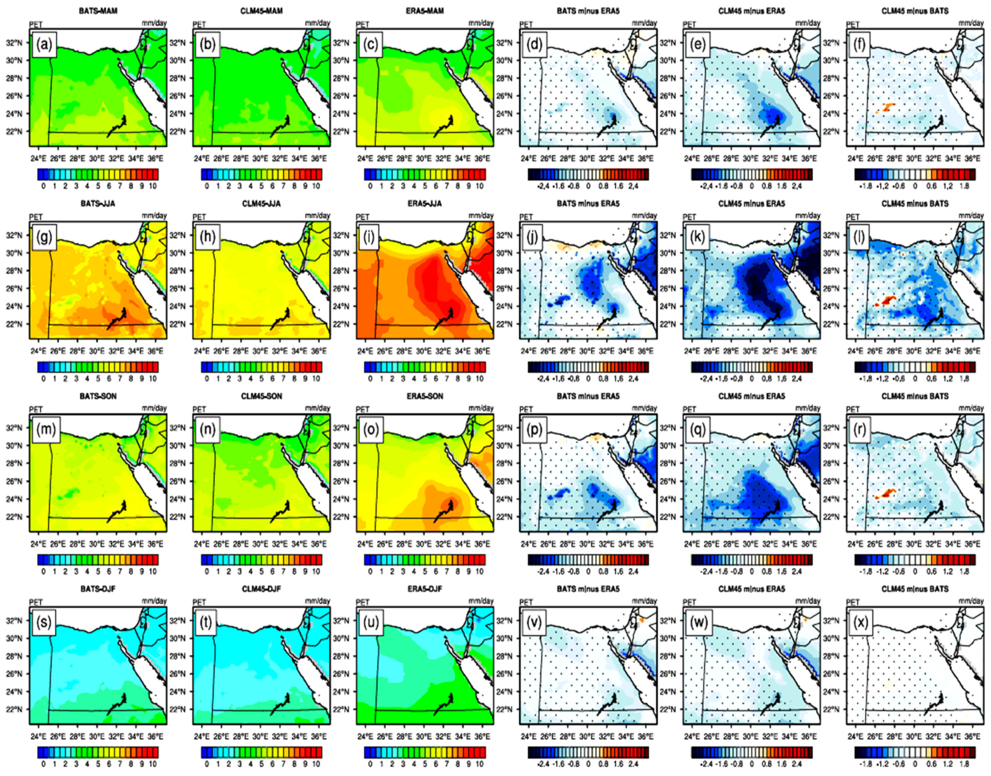
In this section, we investigate the role of land surface parameterization in simulating the PET concerning the ERA5 product. Figure 2 shows the comparison between the BATS and CLM45 (with respect to the ERA5) for the seasons: spring (March–April–May: MAM), summer (June–July–August: JJA), autumn (September–October–November: SON), and winter (December–January–February: DJF). From Figure 2, it can be observed that the RegCM4 was able to reproduce the PET spatial pattern in comparison with the ERA5 in the sense that PET approached its maximum values in JJA, followed by SON and MAM (Figure 2a–c,g–i,m–o). In DJF, the PET had minimum values compared to the other seasons (Figure 2s–u). Also, it can be shown that BATS/CLM45 underestimated the PET compared to the ERA5 (Figure 2d,e,j,k,p,q,v,w). Such behavior can be attributed to the fact that the original version of the temperature-only version of the HS was used (Equation (1)). Another possible reason is that the ERA5 uses the Tiled ECMWF Scheme for Surface Exchanges over Land (TESSEL) land surface model to generate the meteorological variables. In the MAM season, the BATS showed a bias of −0.6 to −1.2 mm day−1; while the CLM45 had a bias of −0.8 to −1.4 mm day−1 (Figure 2d,e).
In the JJA season, the RegCM4’s bias approached its maximum value. For example, the PET bias (induced by the BATS) ranged from −1.5 to −2 mm day−1 (Figure 2j). On the other hand, the PET bias (induced by the CLM45) approached −3 mm day−1 (Figure 2k). In SON, the RegCM4 had a lower bias than that noted in JJA (Figure 2p,q) because the BATS had a bias of −1 to −1.6 mm day−1 (restricted to the area of 22–26° N). Meanwhile, the CLM45 possessed a bias of −0.8 to −2.4 mm day−1 (in the area of 22–28° N). This means that the CLM45 showed a higher bias than the BATS, and its bias pattern had a broader extension than the one noted in the BATS. In DJF, it can be observed that BATS/CLM45 showed a bias of −0.6 to −1 mm day−1 (Figure 2v,w). Also, the PET bias (of the CLM45) showed a broader extension than the one observed in the BATS.
Despite the noted bias, it can be seen that the BATS outperformed the CLM45 in all seasons, particularly in JJA. Such behavior can be attributed to the fact that the BATS overestimated the daily Tmax/Tmin, while the CLM45 underestimated the Tmax/Tmin in comparison with the CRU. Therefore, the BATS succeeded in alleviating the negative bias of the PET (relative to the CLM45) when it was evaluated with the ERA5. Yet, the PET bias (of the BATS) was noted. Therefore, we calibrated the HS equation to possibly reduce the PET bias (see Section 3.2).

3.2. Calibrating the HS Equation

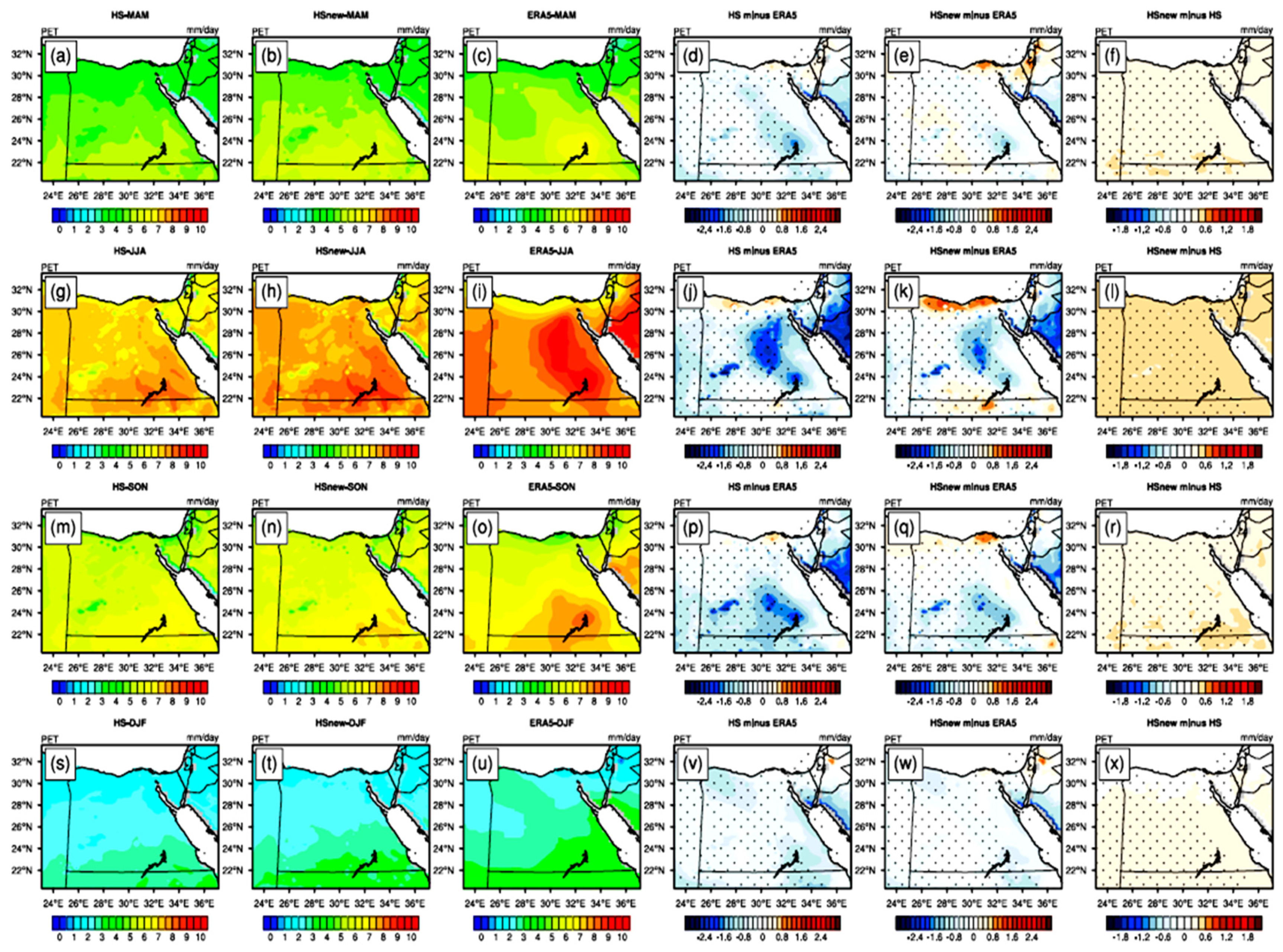
In Section 3.1, it was noted that the BATS had a better performance than the CLM45 compared to the ERA5. Therefore, the BATS scheme was selected to calibrate the HS equation. The old HS equation was designated as HS, while the calibrated version was referred to as HSnew. Figure 3 shows the comparison between the HS and HSnew (concerning the ERA5) for the seasons MAM, JJA, SON, and DJF. The comparison between the HS and HSnew was made with respect to the ERA5 (expressed by bias) and between themselves too (expressed by difference). Both bias/difference were calculated for each grid point using Student’s t-test with alpha equal to 5%. From Figure 3, it can be observed that HSnew succeeded in reducing the PET bias relative to the one noted in the HS. For instance, in the MAM season, the HS showed a bias of −0.6 to −1.2 mm day−1 (Figure 3d). On the other hand, the HSnew had a bias of −0.2 to −0.6 mm day−1 (Figure 3d). From a qualitative point of view, the HSnew had a higher PET than the HS by 0.6 to 0.8 mm day−1 (Figure 3f).
In the JJA season, the HS showed a PET bias of −0.8 to −2.4 mm day−1 (Figure 3j), while the HSnew had a bias of −0.8 to −1.8 mm day−1 (Figure 3k). Also, it can be observed that the HSnew increased the PET by 0.6 to 0.8 mm day−1 relative to the HS (Figure 3l). Both HS/HSnew had a negative bias of the PET in the region of 22–28° N in the SON season (Figure 3p,q). Yet, the PET bias (induced by the HS) was more negative than the one noted in the HSnew. Qualitatively, HSnew had a higher PET (by 0.4 to 0.6 mm day−1 and up to 0.8 mm day−1 in the region of 22–24° N; Figure 3r). Lastly in the DJF season, the HS indicated a PET bias of −0.6 to −1.6 mm day−1 (Figure 3v). Additionally, the HSnew showed a bias of −0.4 to −1 mm day−1 (Figure 3w). Also, the HSnew increased the PET by 0.4 to 0.6 mm day−1 (Figure 3x). It can be noticed that calibrating the HS equation showed its efficiency in the JJA season (where the PET bias was the largest compared to the other seasons), followed by MAM, SON, and finally DJF.

3.3. Boundary Layer Parameterization

The influence of the boundary layer parameterization on the PET is discussed in this section. Similar to Figure 2, the RegCM4 was able to capture the spatial pattern of the PET with respect to the ERA5 in all seasons (Figure 4a–c,g–i,m–o,s–u). Generally, the HOLT showed a positive bias of the PET (about 0.8–1.4 mm day−1) in the MAM, JJA, and SON seasons in the Mediterranean coast (30–32° N; Figure 4d,j,p). Also, the BATS showed a positive bias of 0.4 to 0.6 mm day−1 (in the region of 22–30° N) in the MAM season. In the DJF season, this positive bias was replaced with a negative bias of 0.2–0.4 mm day−1 (Figure 4v). Additionally, a negative bias dominated (0.6 to 1.6 mm day−1) in the region of 24–28° N (see Figure 4d,j,p) in the seasons MAM, JJA, and SON.
Concerning the UW, the situation was different. For example, in the MAM season, the positive bias was 0.6–0.8 mm day−1 in the Mediterranean coast and 0.2–0.4 mm day−1 in the region of 22–30° N (Figure 4e). In the JJA season, the PET bias (in the Mediterranean coast) was less than that noted in the HOLT by 0.4 to 0.6 mm day−1 (Figure 4k,l). Yet, the negative bias (in the region of 24–28° N) was almost similar to the one observed in the HOLT. In addition, the UW succeeded in alleviating the PET bias in the Mediterranean coast (0.6 to 0.8 mm day−1) compared to the noticed bias of the HOLT (0.8 to 1.6 mm day−1) in the SON season (Figure 4q). Finally, in the DJF season, the UW was able to reduce the PET bias (by 0.4 to 0.8 mm day−1; see Figure 4w,x). From a qualitative point of view, it can be observed that UW had a lower PET than HOLT (by 0.4 to 1 mm day−1) in the MAM, JJA, and SON seasons (Figure 4f,l,r).
From Figure 4, it can be seen that the HOLT had a higher PET than UW, particularly in the Mediterranean coast. This noted behavior can be attributed to the fact that the HOLT tends to overestimate the daily temperature, while the UW succeeds in alleviating this warm bias, as reported by [26]. As a result, we selected the UW boundary layer scheme to compare between the two calibrated versions of the HS equation and check which version was the best to compute the PET (see Section 3.4). Compared to the results reported by [26], there was a difference between the HOLT and UW, because the temperature-only version was used. On the other hand, there was no difference noted (between the HOLT and UW) in [26] because the global incident solar radiation was not sensitive to the choice of the boundary layer scheme, and this was the major variable controlling the PET changes followed by the daily mean air temperature.

3.4. Comparison between Two Calibrated Versions of the HS Equation

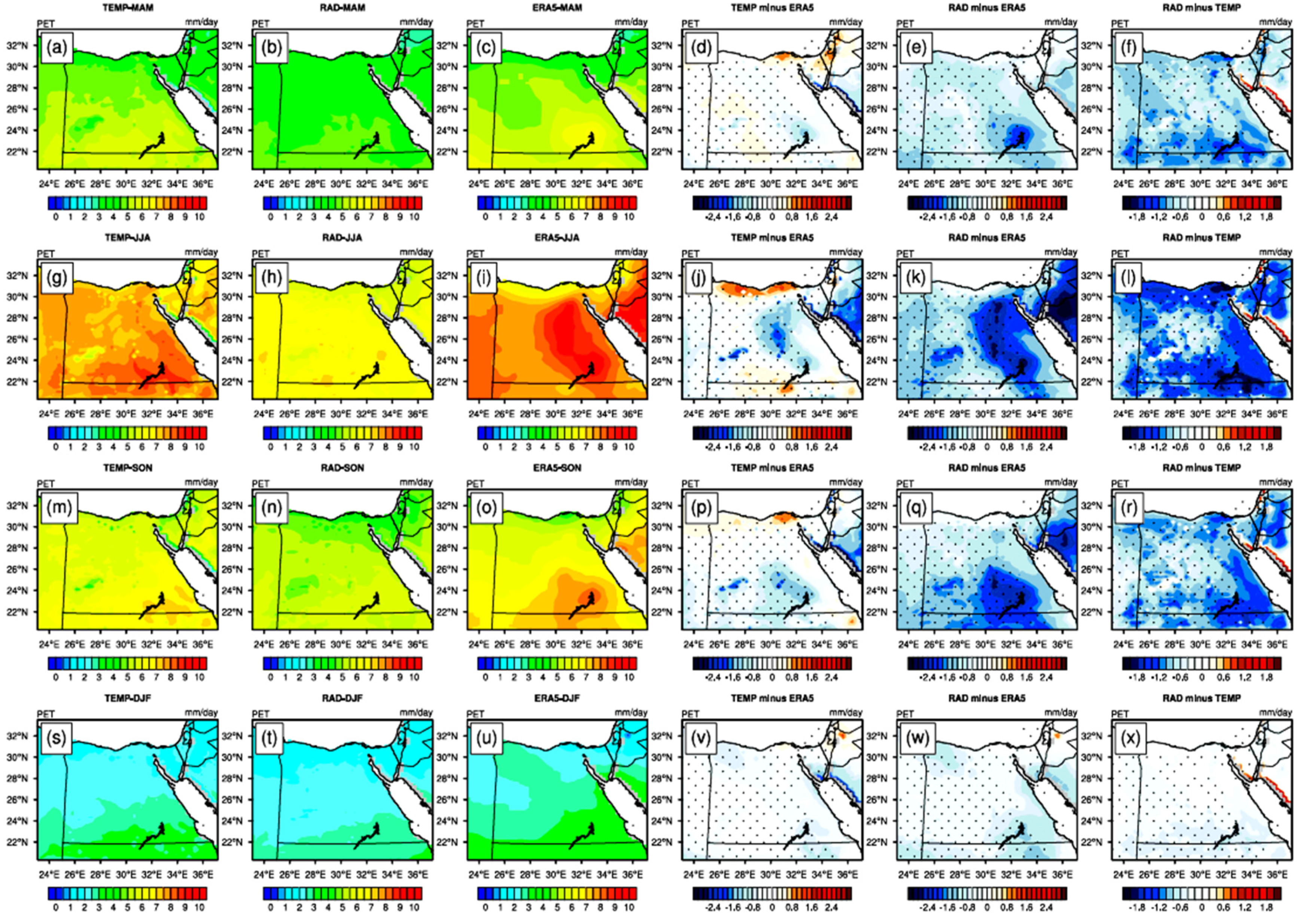
In this section, we compare the two calibrated versions of the HS equations: temperature-only-based formula (TEMP) and temperature-radiation-based formula (RAD) with respect to the ERA5 (Figure 5). Generally, the TEMP and RAD showed a good ability to reproduce the PET pattern concerning the ERA5 in all seasons (Figure 5a–c,g–i,m–o,s–u). Also, the difference between the TEMP and RAD was noted in all seasons. For instance, in the MAM season, the TEMP showed a bias of −0.4 to −0.8 mm day−1, mainly around Lake Nasser (22–24° N; Figure 5d). On the other hand, the RAD had a bias of −0.6 to −1 mm day−1 and −2 mm day−1 around Lake Nasser (Figure 5e). Qualitatively, the RAD was less than the TEMP by 0.4 to 1.4 mm day−1 (Figure 5f). In JJA, the RAD showed a negative bias of −0.6 to 3 mm day−1 (Figure 5k) compared to the RAD that showed a positive bias of 0.6 to 0.8 mm day−1 along the Mediterranean coast and around 1.2 mm day−1 in the region of 24–26° N (Figure 5j). Therefore, the RAD had a lower PET than the TEMP by 1.2 to 2 mm day−1 (Figure 5l). Both the TEMP and RAD had a negative bias in the region of 22 to 26° N, yet the TEMP had a bias of −0.4 to −0.8 mm day−1 and up to −1.2 mm day−1 (along the latitude 24° N) in the SON season (Figure 5p). On the other hand, the RAD showed a bias of −0.8 to −2.6 mm day−1, particularly in the region of 24–26° N (Figure 5q).
In the DJF season, it can be observed that the TEMP had a bias of −0.2 to −0.6 mm day−1 (Figure 5v). On the other hand, the RAD showed a bias of −0.4 to −1 mm day−1 (Figure 5w). Qualitatively, the RAD had a lower PET than the TEMP by 0.2 to 0.4 mm day−1 in the region of 28–32° N and 0.4 to 0.8 mm day−1 in the region of 22–24° N (Figure 5x). Such noted behavior (between TEMP and RAD) can be attributed to the fact that calibrating the radiation coefficient [24] resulted in lower PET values compared to the one noted when the temperature coefficient was tuned (Equation (2)). Among all seasons, it can be observed that the TEMP outperformed the RAD in comparison with the ERA5. Because of the noted biases in the TEMP, the LS bias-correction was applied, evaluated, and validated concerning the ERA5 (Section 3.5).

3.5. Bias-Correcting the PET

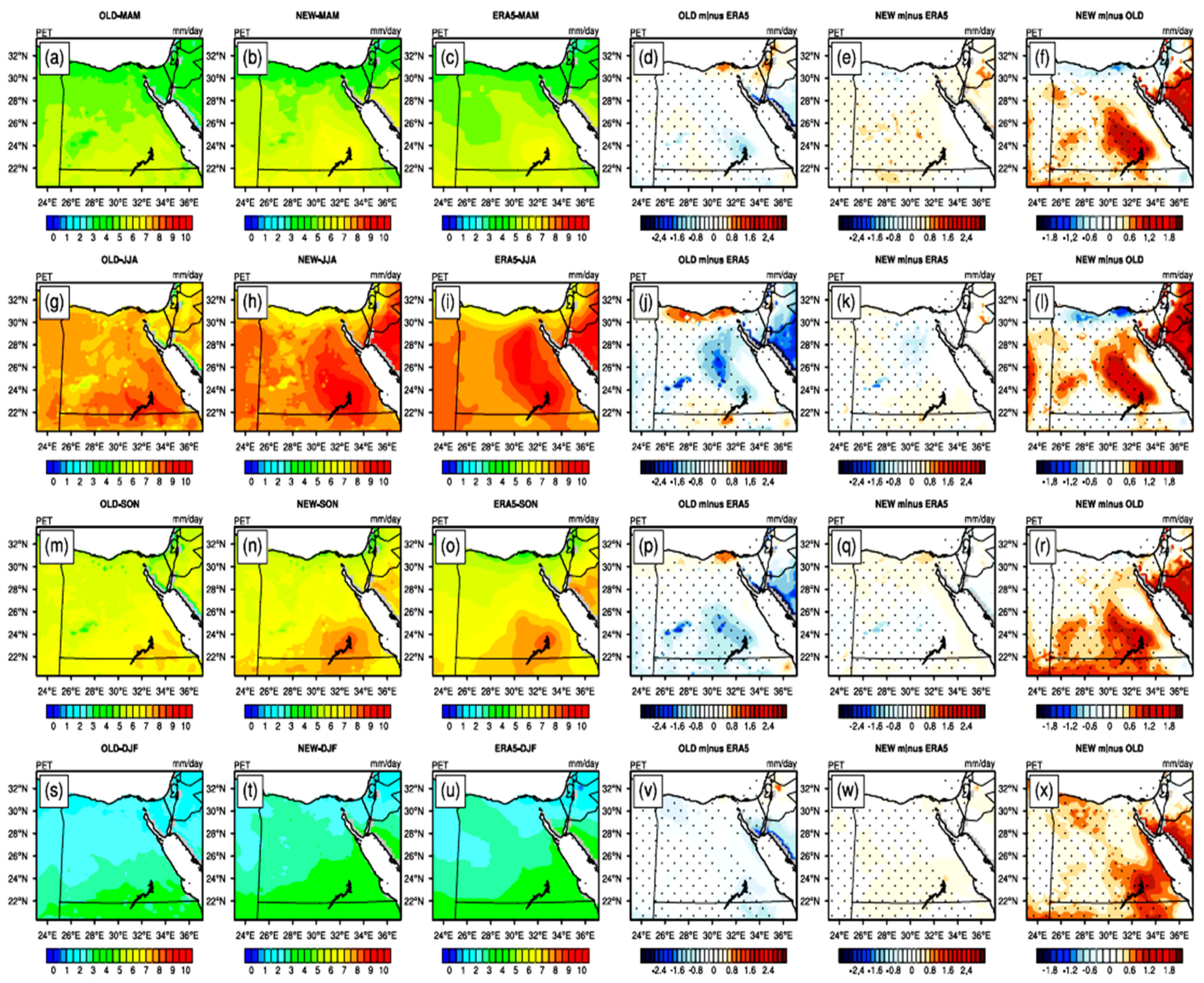
In Section 3.4, it was noted that TEMP exhibited biases, particularly in the JJA and SON seasons. Therefore, the LS bias-correction was applied to the RegCM4’s output. For the LS to be evaluated, the period 1981–2010 was divided to two segments: 1981–1996 as the evaluation period and 1997–2010 as the validation period. Then, the climatological bias (between the ERA5 and TEMP) for each season was calculated for the period 1981–1996, which was added to the periods 1981–1996 (to check the added value of the LS in the evaluation period) and 1997–2010 (to see if the climatological bias factor can be applied to any time segment outside the evaluation period). Figure 6 shows the TEMP before applying the LS (OLD) and after applying the LS (NEW) in comparison with the ERA5 in the period 1981–1996. In the MAM season, it can be noted that the OLD experienced a negative bias of 0.6 to 1 mm day−1 in the region of 22–30° N and a positive bias of 0.8 to 1 mm day−1 in the delta region (approximately 31° N; Figure 6d). On the other hand, the NEW showed a positive bias of 0.4 to 0.6 mm day−1 (Figure 6e). Qualitatively, the NEW was higher than the OLD by 0.4 to 1.2 mm day−1 (and in the area 22–26° N 1.6 mm day−1; see Figure 6f).
In the JJA and SON seasons, the efficiency of the LS (to reduce the PET bias) can be observed. For instance, the OLD showed a positive bias of 0.8 to 1.2 mm day−1 in the Mediterranean coast and a negative bias of 0.8 to 1.8 mm day−1 in the region of 24 to 28° N in the JJA season (Figure 6j). In the NEW, it can be noticed that the PET bias (in the Mediterranean coast) had disappeared. Additionally, the noted PET negative bias (in the region of 24 to 28° N) became 0.4 to 0.8 mm day−1 (Figure 6k). In other ways, the NEW had a higher PET than the OLD by 0.6 to 1.6 mm day−1 (see Figure 6l). In the SON season, it can be observed that the OLD showed a positive PET bias (in the delta region) of 0.8 to 1 mm day−1, while it had a negative PET bias of 0.8 to 1.8 mm day−1 (in the region 22–26° N; Figure 6p). When the LS was applied, the NEW showed a positive bias of 0.2 to 0.4 mm day−1 (and 0.6 to 0.8 mm day−1 in the delta region; Figure 6q). The bottom line is that the NEW was higher than the OLD by 0.4 to 1.8 mm day−1 (particularly in the region 22–26° N; Figure 6r). Lastly, in the DJF season, the noted negative bias of the OLD (0.6 to 1 mm day−1; Figure 6v) was replaced by a positive bias of 0.2 to 0.4 mm day−1 in the NEW (Figure 6w). Qualitatively, the NEW had a higher PET by 0.4 to 1.6 mm day−1, particularly around Lake Nasser (Figure 6x).
From Figure 6, the NEW not only succeeded in reducing the PET bias (in comparison with the ERA5), but also showed a better ability to capture the PET spatial pattern (than the OLD) with respect to the ERA5 (Figure 6a–c,g–i,m–o,s–u). The next step was to validate the LS outside the evaluation period. Figure 7 shows the comparison between the OLD and NEW (in the validation period 1997–2010) concerning the ERA5. From Figure 7, we can observe the added value of the LS in the validation period. For instance, in the MAM season, the OLD showed a PET bias of −0.6 to −1 mm day−1 (particularly in the region of 22–24° N; Figure 7d). On the other hand, the NEW had a PET bias of +0.2 to +0.4 mm day−1 (Figure 7e). Also, the NEW was higher than the OLD by 0.4 to 1.6 mm day−1 (Figure 7f). In the JJA season, it can be seen that the LS showed its potential skills in reducing the PET bias. For example, the OLD exhibited a positive bias of 0.6 to 1 mm day−1 along the Mediterranean coast and a negative bias of 0.6 to 2.4 mm day−1 elsewhere (Figure 7j).
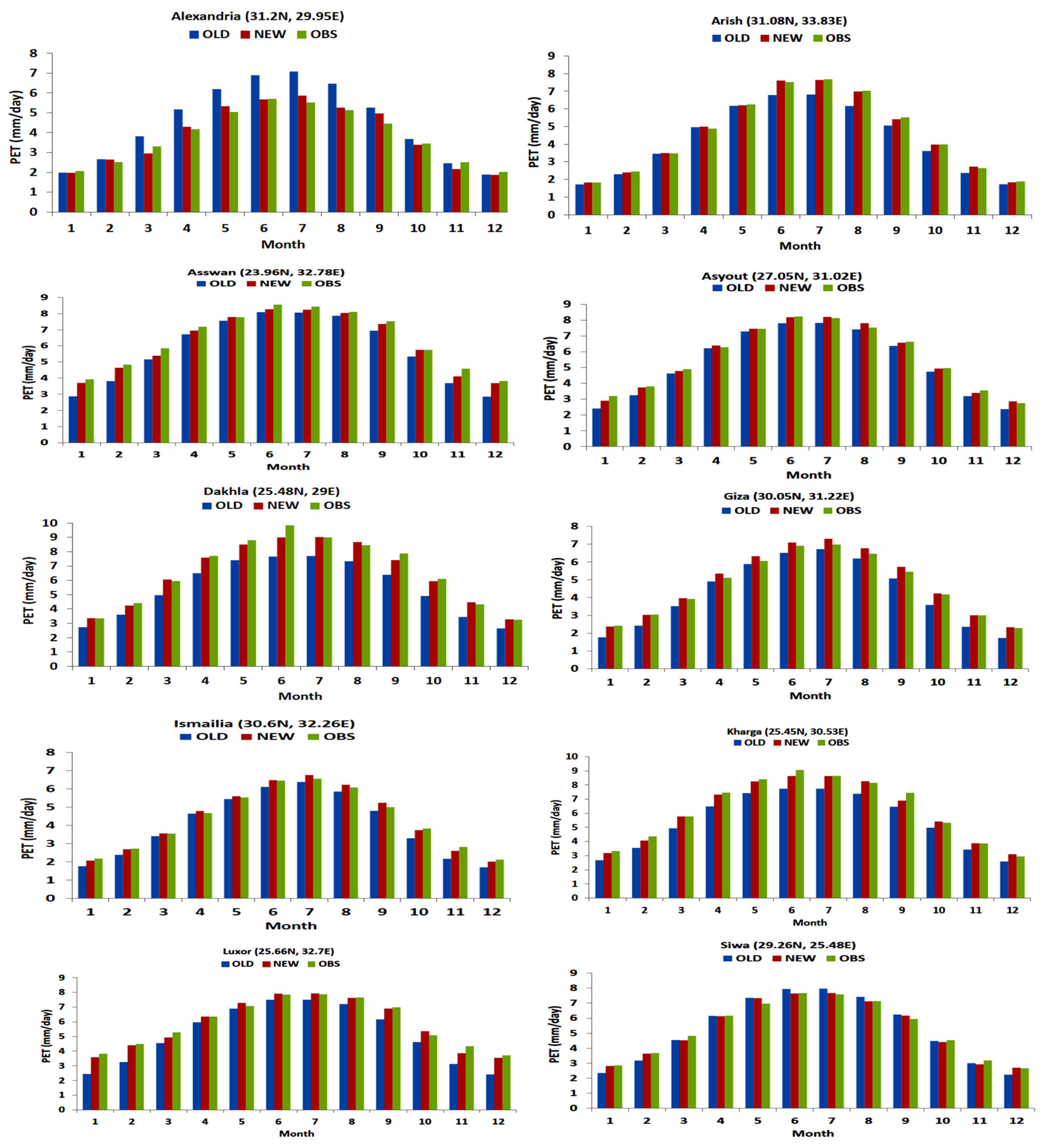
On the other hand, the NEW had a negative PET bias of 0.4 to 0.8 mm day−1 (Figure 7k). Therefore, it can be noticed that the NEW had a higher PET than the OLD by 0.6 to 1.4 mm day−1 (Figure 7l). In the SON season, it can be observed that the OLD had a negative bias of 0.6 to 1.8 mm day−1 (Figure 7p). Additionally, the NEW showed a PET bias of +0.2 mm day−1 (Figure 7q). Also, the NEW was higher than the OLD by 0.4 to 1.6 mm day−1 (Figure 7r). The same behavior was noted in the DJF season (see Figure 7v–x). From Figure 6 and Figure 7, it can be observed that the LS succeeded in reducing the PET bias either in the evaluation or the validation periods. To further evaluate the potential skills of the LS (in the validation period), a climatological annual cycle was plotted (before and after applying the LS) with respect to the ERA5 for the ten locations (indicated in Figure 1). Also, the Taylor diagram was used to quantify the performance of the RegCM4 for the ten locations (see Section 3.6).

3.6. Climatological Annual Cycle

Figure 8 shows the ERA5-PET (OBS) climatological annual cycle of the ten locations (see Figure 1) in the period 1981–2010. From Figure 8, it can be observed that the PET showed a gradient where Alexandria showed low PET values compared to Kharga (where PET values were high). That is, the PET amplitude was minimized in Alexandria and maximized in Dakhla. This noted behavior can be explained by the fact that Alexandria lies on the Mediterranean coast (receiving low incident solar radiation with high cloud cover), while Dakhla lies in the western desert (receiving high incident solar radiation with low cloud cover). Among the ten locations, Arish possessed the minimum PET values in January, February, and December. On the other hand, Alexandria had minimum PET records from March until November. Concerning the maximum PET values, Asswan constituted the months January, February, November, and December. Additionally, Dakhla possessed the maximum PET values from March to October.
For each location, maximum/minimum PET values vary with the month. For instance, in Arish, Giza, Ismailia, and Luxor, maximum PET values can be found in July. For the other locations, maximum PET values can be seen in June. Also, Arish has minimum PET values in January, while the other locations show minimum PET values in December. To further evaluate the performance of the RegCM4 in the validation period (Section 3.5), the PET climatological annual cycle was plotted with respect to the ERA5 (Figure 9). From Figure 9, it can be seen the NEW was closer to the OBS than the OLD. Such performance depends on the location and month. For instance, in Alexandria, it can be observed that both OLD and NEW were close to the OBS in January, February, and December. Also, OLD was closer to the OBS than the NEW in March and November. On the other hand, NEW outperformed the OLD during rest of months.
In Arish, both the OLD and NEW matched the OBS values in January to May and December, while the NEW outperformed the OLD during the rest of the months. Also, the NEW showed a better performance than the OLD (with respect to the OBS) in all months in Asswan, particularly during January, February, November, and December. Among the other locations, it can be observed that the NEW showed a superior performance (compared to the OLD) concerning the OBS.
Additionally, performance of the OLD/NEW (with respect to the OBS) was quantified using the Taylor diagram. Figure 10 shows the Taylor diagram exploring the performance of the OLD/NEW for the ten locations. From Figure 10, it can be noticed that both the OLD and NEW had a high CC (ranging from 0.96 to 0.998). Also, the Bias was between 1 and 5% (for the OLD) and less than 1% (for the NEW). Additionally, they differed in the Ratio. For example, in the OLD, the Ratio lay between 0.84 and 1.43, while the NEW ranged between 0.94 and 1.12.

4. Discussion and Conclusions

Potential evapotranspiration (PET) is an important variable for monitoring the daily crop water needs and for drought assessment [9]. Also, it is an essential input in the hydrological models. Therefore, it is necessary to accurately estimate the PET. The Penman–Monteith method is the major method (PM; recommended by the FAO) to compute the PET. However, the authors of [8] reported that the PM does not work properly with an unlimited supply of the soil moisture and very dry conditions. Additionally, the PM method involves many variables that contribute to an increased uncertainty in the calculated reference evapotranspiration [24]. Therefore, a simple empirical method is needed and to be calibrated with respect to the observations of the PM.
Among the available empirical methods, the Hargreaves and Samani (HS) method was recommended (after the PM method). The HS has proven its efficiency in estimating the PET in various regions across the globe [7,10,17,21]. Regional climate models (RCMs) are useful tools to compute the PET at any grid point or under different warming future scenarios. For example, the authors of [21] used different RCMs (and their ensemble average) to estimate the PET (by means of the HS equation) in Southern Spain. Also, they highlighted the added value of calibrating the coefficients of the HS to accurately calculate the PET with respect to PM observations. Furthermore, the authors of [23] used the RegCM4 regional climate model and the HS to estimate the water loss of Egypt under the RCP4.5 future scenario.
Additionally, the authors of [24] used the RegCM4 to investigate the sensitivity of the PET to different lateral boundary conditions. Also, they highlighted the added value of using the HS (and its calibrated version) to compute the PET in comparison with ERA5 observations. Until the present day, and to the best of our knowledge, no study has specifically investigated the impact of various physical schemes (which influence the meteorological inputs used in the Hargreaves and Samani equation) in arid regions such as Egypt.
Therefore, it was necessary to explore this point to understand how the physical schemes can affect the PET. For instance, the authors of [26] concluded that the UW boundary layer scheme outperforms the HOLT (concerning the daily mean air temperature) in comparison with the ERA5. Also, the authors of [32] used the RegCM4 model to investigate the role of the land surface parameterization in simulating the daily maximum and minimum air temperature (Tmax/Tmin) with respect to the CRU and station data. They observed that the CLM45 land surface model is the suitable scheme to simulate Tmax and Tmin.
In the present study, we examined the role of land surface and boundary layer parameterizations in simulating the PET. The added value of calibrating the HS equation and adopting the LS bias-correction method was also investigated. To achieve this task, four simulations were conducted in the period of 1979 to 2010 and configured with 25 km grid spacing. The ERA5-land-based product (hPET; ERA5 for short) was used as the observational dataset to evaluate the RegCM4 model performance for each grid point as well as for specific locations (see Figure 1). The results of this study can be summarized as follows:
  • With respect to the ERA5, the BATS outperformed the CLM45, and the UW was better than the HOLT in all seasons concerning the PET.
  • Calibrating the temperature coefficient (of the HS equation) succeeded in reducing the PET bias in comparison with the ERA5.
  • Comparison between the two calibrated versions of the HS revealed that the temperature-only version provided a lower PET bias compared to the one noted in the radiation-temperature version.
  • The LS method explored its added value in reducing the PET bias either in the evaluation or the validation period.
  • Concerning the climatological annual cycle, the calibrated HS equation provided a better performance than the original version (in the ten locations) in comparison with the ERA5.
Therefore, it can be concluded that the RegCM4 can be used to estimate the PET of Egypt using the BATS land surface model, the UW boundary layer scheme, and the LS bias-correction method either in the present climate or under different future scenarios from the pool of the Coupled Model Intercomparison Project Phase 6 (CMIP6). It is important to highlight that the current study relied on using one regional climate model and the bias-correction method. Therefore, a future work will manipulate an ensemble of the regional climate models following [22] and compare between different techniques of the bias-correction [61,62]. Also, a comparison between the hydrostatic core of the RegCM4 [45] and non-hydrostatic of the RegCM5 [48] will be performed to check if the PET can be affected by the hydrostatic regime.

Author Contributions

Conceptualization, S.A.A.; methodology, S.A.A.; software, S.A.A.; validation, S.A.A.; formal analysis, S.A.A. and C.F.O.; investigation, S.A.A. and C.F.O.; resources, S.A.A.; data curation, S.A.A.; writing—original draft preparation, S.A.A. and C.F.O.; writing—review and editing, S.A.A. and C.F.O.; visualization, S.A.A. and C.F.O.; supervision, S.A.A. and C.F.O.; project administration, S.A.A. All authors have read and agreed to the published version of the manuscript.

Funding

This research received no external funding.

Data Availability Statement

Data are contained within the article.

Acknowledgments

The Egyptian Meteorological Authority (EMA) is acknowledged for providing the computational power to conduct the model simulations. Hourly potential evapotranspiration (hPET) was retrieved from the web link https://data.bris.ac.uk/data/dataset/qb8ujazzda0s2aykkv0oq0ctp (accessed on 18 October 2022). However, the monthly mean can be acquired from the authors upon request. ERA-Interim reanalysis was retrieved from the ICTP data web link http://clima-dods.ictp.it/Data/RegCM_Data/EIN15 (accessed on 18 October 2022).

Conflicts of Interest

The authors declare no conflicts of interest.

References

  1. Currie, D.J. Energy and large-scale patterns of animal and plant species richness. Am. Nat. 1991, 137, 27–49. [Google Scholar] [CrossRef]
  2. Allen, G.R.; Pereira, S.L.; Raes, D.; Smith, M. Crop Evapotranspiration: Guidelines for Computing Crop Water Requirements; Report 56; Food and Agricultural Organization of the United Nations (FAO): Rome, Italy, 1998; 300p. [Google Scholar]
  3. Li, Z.; Yang, Y.; Kan, G.; Hong, Y. Study on the Applicability of the Hargreaves Potential Evapotranspiration Estimation Method in CREST Distributed Hydrological Model (Version 3.0) Applications. Water 2018, 10, 1882. [Google Scholar] [CrossRef]
  4. Hamed, M.M.; Iqbal, Z.; Nashwan, M.S.; Kineber, A.F.; Shahid, S. Diminishing evapotranspiration paradox and its cause in the Middle East and North Africa. Atmos. Res. 2023, 289, 106760. [Google Scholar] [CrossRef]
  5. Nooni, I.K.; Hagan, D.F.T.; Wang, G.; Ullah, W.; Lu, J.; Li, S.; Dzakpasu, M.; Prempeh, N.A.; Lim Kam Sian, K.T.C. Future Changes in Simulated Evapotranspiration across Continental Africa Based on CMIP6 CNRM-CM6. Int. J. Environ. Res. Public Health 2021, 18, 6760. [Google Scholar] [CrossRef]
  6. Zhang, Y.; Fu, B.; Feng, X.; Pan, N. Response of Ecohydrological Variables to Meteorological Drought under Climate Change. Remote Sens. 2022, 14, 1920. [Google Scholar] [CrossRef]
  7. Murat, C.; Hatice, C.; Tefaruk, H.; Kisi, O. Modifying Hargreaves–Samani equation with meteorological variables for estimation of reference evapotranspiration in Turkey. Hydrol. Res. 2017, 48, 480–497. [Google Scholar] [CrossRef]
  8. Brutsaert, W.; Parlange, M.B. Hydrologic cycle explains the evaporation paradox. Nature 1998, 396, 30. [Google Scholar] [CrossRef]
  9. Spinoni, J.; Barbosa, P.; Bucchignani, E.; Cassano, J.; Cavazos, T.; Cescatti, A.; Christensen, J.H.; Christensen, O.B.; Coppola, E.; Evans, J.P.; et al. Global exposure of population and land-use to meteorological droughts under different warming levels and SSPs: A CORDEX-based study. Int. J. Climatol. 2021, 41, 6825–6853. [Google Scholar] [CrossRef]
  10. Raziei, T.; Pereirab, L.S. Estimation of ETo with Hargreaves–Samani and FAO-PM temperature methods for a wide range of climates in Iran. Agric. Water Manag. 2013, 121, 1–18. [Google Scholar] [CrossRef]
  11. Hargreaves, G.H.; Samni, Z.A. Reference crop evapotranspiration from temperature. Appl. Eng. Agric. 1985, 1, 96–99. [Google Scholar] [CrossRef]
  12. Hargreaves, G.L.; Allen, R.G. History and evaluation of Hargreaves evapotranspiration equation. J. Irrigat. Drain. Eng. 2003, 129, 53–63. [Google Scholar] [CrossRef]
  13. Priestley, C.H.B.; Taylor, R.J. On the assessment of surface heat flux and evaporation using large-scale parameters. Mon. Weather Rev. 1972, 100, 81–92. [Google Scholar] [CrossRef]
  14. Rohwer, C. Evaporation from free water surface. USDA Tech. Null. 1931, 217, 1–96. [Google Scholar]
  15. Mohammadieh, M.; Noori, M.; Helali, J.; Nazari, B.; Sohrabi, T. Evaluation of Hargreaves equation for calculating daily ETo (Case study: North West of Iran). Adv. Nat. Appl. Sci. 2009, 3, 273–279. [Google Scholar]
  16. Rajabi, A.; Babakhani, Z. The study of potential evapotranspiration in future periods due to climate change in west of Iran. Int. J. Clim. Chang. Strateg. Manag. 2018, 10, 161–177. [Google Scholar] [CrossRef]
  17. Srivastava, A.; Sahoo, B.; Raghuwanshi, N.S.; Chatterjee, C. Modelling the dynamics of evapotranspiration using Variable Infiltration Capacity model and regionally calibrated Hargreaves approach. Irrig. Sci. 2018, 36, 289–300. [Google Scholar] [CrossRef]
  18. Swain, R.; Sahoo, B. Improving river water quality monitoring using satellite data products and a genetic algorithm processing approach. Sustain. Water Qual. Ecol. 2017, 9–10, 88–114. [Google Scholar] [CrossRef]
  19. Er-Raki, S.; Chehbouni, A.; Khabba, S.; Simonneaux, V.; Jarlan, L.; Ouldbba, A.; Rodriguez, J.C.; Allen, R. Assessment of reference evapotranspiration methods in semi-arid regions: Can weather forecast data be used as alternate of ground meteorological parameters? J. Arid. Environ. 2010, 74, 1587–1596. [Google Scholar] [CrossRef]
  20. Elagib, N.A.; Musa, A.A. Correcting Hargreaves-Samani formula using geographical coordinates and rainfall over different timescales. Hydrol. Process. 2022, 37, e14790. [Google Scholar] [CrossRef]
  21. Giménez, P.O.; García-Galiano, S.G. Assessing Regional Climate Models (RCMs) Ensemble-Driven Reference Evapotranspiration over Spain. Water 2018, 10, 1181. [Google Scholar] [CrossRef]
  22. Giorgi, F.; Coppola, E.; Solmon, F.; Mariotti, L.; Sylla, M.B.; Bi, X.; Elguindi, N.; Diro, G.T.; Nair, V.; Giuliani, G.; et al. RegCM4: Model description and preliminary tests over multiple CORDEX domains. Clim. Res. 2012, 52, 7–29. [Google Scholar] [CrossRef]
  23. Abdel Wahab, M.M.; Essa, Y.H.; Khalil, A.A.; Elfadli, K.; Giulia, P. Water Loss in Egypt Based on the Lake Nasser Evaporation and Agricultural Evapotranspiration. Environ. Asia 2018, 11, 192–204. [Google Scholar] [CrossRef]
  24. Anwar, S.A.; Lazić, I. Estimating the Potential Evapotranspiration of Egypt Using a Regional Climate Model and a High-Resolution Reanalysis Dataset. Environ. Sci. Proc. 2023, 25, 29. [Google Scholar] [CrossRef]
  25. Anwar, S.A.; Srivastava, A. On the Sensitivity of Potential Evapotranspiration in Egypt to Different Dynamical Downscaling Options and Boundary Layer Schemes Using a High-Resolution Regional Climate Model. Eng. Proc. 2023, 56, 116. [Google Scholar] [CrossRef]
  26. Anwar, S.A.; Mostafa, S.M. On the Sensitivity of the Daily Mean Air Temperature of Egypt to Boundary Layer Schemes Using a High-Resolution Regional Climate Model (RegCM4). J. Biomed. Res. Environ. Sci. 2023, 4, 474–484. [Google Scholar] [CrossRef]
  27. Holtslag, A.A.M.; Boville, B.A. Local versus nonlocal boundary layer diffusion in a global model. J. Clim. 1993, 6, 1825–1842. [Google Scholar] [CrossRef]
  28. Grenier, H.; Bretherton, C.S. A moist PBL parameterization for large scale models and its application to subtropical cloud topped marine boundary layers. Mon. Weather Rev. 2001, 129, 357–377. [Google Scholar] [CrossRef]
  29. Hersbach, H.; Bell, B.; Berrisford, P.; Hirahara, S.; Horanyi, A.; Muñoz-Sabater, J.; Nicolas, J.; Peubey, C.; Radu, R.; Schepers, D.; et al. The ERA5 global reanalysis. Q. J. R. Meteorol. Soc. 2020, 146, 1999–2049. [Google Scholar] [CrossRef]
  30. Anwar, S.A.; Mostafa, S.M. Assessment of the Sensitivity of Daily Maximum and Minimum Air Temperatures of Egypt to Soil Moisture Status and Land Surface Parameterization Using RegCM4. Eng. Proc. 2023, 56, 115. [Google Scholar] [CrossRef]
  31. Oleson, K.W.; Lawrence, D.M.; Bonan, G.B.; Drewniak, B.; Huang, M.; Koven, C.D.; Levis, S.; Li, F.; Riley, W.J.; Subin, Z.M.; et al. Technical Description of Version 4.5 of the Community Land Model (CLM); NCAR Technical Note NCAR/TN-503+STR; National Center for Atmospheric Research: Boulder, CO, USA, 2013. [Google Scholar] [CrossRef]
  32. Dickinson, R.E.; Henderson-Sellers, A.; Kennedy, P.J. Biosphere-Atmosphere Transfer Scheme (BATS) Version 1e as Coupled to the NCAR Community Climate Model (No. NCAR/TN-387+STR); University Corporation for Atmospheric Research: Boulder, CO, USA, 1993. [Google Scholar] [CrossRef]
  33. Singer, M.; Asfaw, D.; Rosolem, R.; Cuthbert, M.O.; Miralles, D.G.; MacLeod, D.; Michaelides, K. Hourly potential evapotranspiration (hPET) at 0.1degs grid resolution for the global land surface from 1981-present. Sci. Data 2021, 8, 224. [Google Scholar] [CrossRef] [PubMed]
  34. Peel, M.C.; Finlayson, B.L.; McMahon, T.A. Updated World Map of the Köppen-Geiger Climate Classification. Hydrol. Earth Syst. Sci. 2007, 11, 1633–1644. [Google Scholar] [CrossRef]
  35. El Kenawy, A.; Lopez-Moreno, J.I.; Vicente-Serrano, S.M.; Morsi, F. Climatological modeling of monthly air temperature and precipitation in Egypt through GIS techniques. Clim. Res. 2010, 42, 161–176. [Google Scholar] [CrossRef]
  36. Nashwan, M.S.; Shahid, S.; Chung, E.-S. High-Resolution Climate Projections for a Densely Populated Mediterranean Region. Sustainability 2020, 12, 3684. [Google Scholar] [CrossRef]
  37. Hamed, M.M.; Nashwan, M.S.; Shahid, S. Inter-comparison of Historical Simulation and Future Projection of Rainfall and Temperature by CMIP5 and CMIP6 GCMs Over Egypt. Int. J. Climatol. 2022, 42, 4316–4332. [Google Scholar] [CrossRef]
  38. Hamed, M.M.; Nashwan, M.S.; Shiru, M.S.; Shahid, S. Comparison between CMIP5 and CMIP6 Models over MENA Region Using Historical Simulations and Future Projections. Sustainability 2022, 14, 10375. [Google Scholar] [CrossRef]
  39. Mostafa, S.M.; Anwar, S.A.; Zakey, A.S.; Wahab, M.M.A. Bias-correcting the maximum and minimum air temperatures of Egypt using a high-resolution Regional Climate Model (RegCM4). Eng. Proc. 2023, 31, 73. [Google Scholar] [CrossRef]
  40. Dickinson, R.E.; Errico, R.M.; Giorgi, F.; Bates, G.T. A regional climate model for the western United States. Clim. Chang. 1989, 15, 383–422. [Google Scholar] [CrossRef]
  41. Giorgi, F.; Bates, G.T. The climatological skill of a regional model over complex terrain. Mon. Weather Rev. 1989, 117, 2325–2347. [Google Scholar] [CrossRef]
  42. Giorgi, F. Thirty years of regional climate modeling: Where are we and where are we going? J. Geophys. Res. 2019, 124, 5696–5723. [Google Scholar] [CrossRef]
  43. Giorgi, F.; Marinucci, M.R.; Bates, G.T. Development of a second generation regional climate model (RegCM2). Part I: Boundary layer and radiative transfer processes. Mon. Weather Rev. 1993, 121, 2794–2813. [Google Scholar] [CrossRef]
  44. Giorgi, F.; Marinucci, M.R.; Bates, G.T.; DeCanio, G. Development of a second generation regional climate model (RegCM2). Part II: Convective processes and assimilation of lateral boundary conditions. Mon. Wea. Rev. 1993, 121, 2814–2832. [Google Scholar] [CrossRef]
  45. Pal, J.S.; Giorgi, F.; Bi, X.; Elguindi, N.; Solmon, F.; Gao, X.; Rauscher, S.A.; Francisco, R.; Zakey, A.; Winter, J.; et al. The ICTP RegCM3 and RegCNET: Regional climate modeling for the developing World. Bull. Amer. Meteor. Soc. 2007, 88, 1395–1409. [Google Scholar] [CrossRef]
  46. Giorgi, F.; Coppola, E.; Giuliani, G.; Ciarlo‘, J.M.; Pichelli, E.; Nogherotto, R.; Raffaele, F.; Malguzzi, P.; Davolio, S.; Stocchi, P.; et al. The Fifth Generation Regional Climate Modeling System, RegCM5: Description and Illustrative Examples at Parameterized Convection and Convection-Permitting Resolutions. J. Geophys. Res. Atmos. 2023, 128, e2022JD038199. [Google Scholar] [CrossRef]
  47. Coppola, E.; Stocchi, P.; Pichelli, E.; Torres Alavez, J.A.; Glazer, R.; Giuliani, G.; Di Sante, F.; Nogherotto, R.; Giorgi, F. Non-Hydrostatic RegCM4 (RegCM4-NH): Model description and case studies over multiple domains. Geosci. Model. Dev. 2021, 14, 7705–7723. [Google Scholar] [CrossRef]
  48. Kiehl, J.T.; Hack, J.; Bonan, G.; Boville, B.; Breigleb, B.; Williamson, D.; Rasch, P. Description of the Ncar Community Climate Model (ccm3), National Center for Atmospheric Research Technical Note NCAR/TN-420+STR; National Center for Atmospheric Research: Boulder, CO, USA, 1996; 95p. [Google Scholar]
  49. Mlawer, E.J.; Taubman, S.J.; Brown, P.D.; Iacono, M.J.; Clough, S.A. Radiative transfer for inhomogenoeus atmoshere: RRTM, a validated correlated-k model for the longwave. J. Geophys. Res. 1997, 102, 16663–16682. [Google Scholar] [CrossRef]
  50. Emanuel, K.A.; Zivkovic-Rothman, M. Development and evaluation of a convection scheme for use in climate models. J. Atmos. Sci. 1999, 56, 1766–1782. [Google Scholar] [CrossRef]
  51. Dee, D.P.; Uppala, S.M.; Simmons, A.J.; Berrisford, P.; Poli, P.; Kobayashi, S.; Andrae, U.; Balmaseda, M.A.; Balsamo, G.; Bauer, P.; et al. The ERA-Interim reanalysis: Configuration and performance of the data assimilation system. Q. J. R. Meteorol. Soc. 2011, 137, 553–597. [Google Scholar] [CrossRef]
  52. Steiner, A.L.; Pal, J.S.; Rauscher, S.A.; Bell, J.L.; Diffenbaugh, N.S.; Boone, A.; Sloan, L.C.; Giorgi, F. Land surface coupling in regional climate simulations of the West African monsoon. Clim. Dyn. 2009, 33, 869–892. [Google Scholar] [CrossRef]
  53. Dorigo, W.; Wagner, W.; Albergel, C.; Albrecht, F.; Balsamo, G.; Brocca, L.; Chung, D.; Ertl, M.; Forkel, M.; Gruber, A.; et al. ESA CCI Soil Moisture for improved Earth system understanding: State-of-the art and future directions. Remote Sens. Environ. 2017, 203, 185–215. [Google Scholar] [CrossRef]
  54. Gruber, A.; Scanlon, T.; van der Schalie, R.; Wagner, W.; Dorigo, W. Evolution of the ESA CCI Soil Moisture climate data records and their underlying merging methodology. Earth Syst. Sci. Data. 2019, 11, 717–739. [Google Scholar] [CrossRef]
  55. Teutschbein, C.; Seibert, J. Bias correction of regional climate model simulations for hydrological climate-change impact studies: Review and evaluation of different methods. J. Hydrol. 2012, 456–457, 12–29. [Google Scholar] [CrossRef]
  56. Daniel, H. Performance assessment of bias correction methods using observed and regional climate model data in different watersheds, Ethiopia. J. Water Clim. 2023, 14, 2007–2028. [Google Scholar] [CrossRef]
  57. Lafon, T.; Dadson, S.; Buys, G.; Prudhomme, C. Bias correction of daily precipitation simulated by a regional climate model: A comparison of methods. Int. J. Climatol. 2013, 33, 1367–1381. [Google Scholar] [CrossRef]
  58. Taylor, K.E. Summarizing multiple aspects of model performance in a single diagram. J. Geophys. Res. Atmos. 2001, 106, 7183–7192. [Google Scholar] [CrossRef]
  59. Baker, N.C.; Taylor, P.C. A Framework for Evaluating Climate Model Performance Metrics. J. Clim. 2016, 29, 1773–1782. [Google Scholar] [CrossRef]
  60. Perez, J.; Menendez, M.; Mendez, F.J.; Losada, I.J. Evaluating the performance of CMIP3 and CMIP5 global climate models over the north-east Atlantic region. Clim. Dyn. 2014, 43, 2663–2680. [Google Scholar] [CrossRef]
  61. Chen, H.; Zhu, G.; Zhang, K.; Bi, J.; Jia, X.; Ding, B.; Zhang, Y.; Shang, S.; Zhao, N.; Qin, W. Evaluation of Evapotranspiration Models Using Different LAI and Meteorological Forcing Data from 1982 to 2017. Remote Sens. 2020, 12, 2473. [Google Scholar] [CrossRef]
  62. Martens, B.; Miralles, D.G.; Lievens, H.; van der Schalie, R.; de Jeu, R.A.M.; Fernández-Prieto, D.; Beck, H.E.; Dorigo, W.A.; Verhoest, N.E.C. GLEAM v3: Satellite-based land evaporation and root-zone soil moisture. Geosci. Model. Dev. 2017, 10, 1903–1925. [Google Scholar] [CrossRef]
  63. Harris, I.; Osborn, T.J.; Jones, P.; Lister, D. Version 4 of the CRU TS monthly high-resolution gridded multivariate climate dataset. Sci. Data 2020, 7, 109. [Google Scholar] [CrossRef]
  64. Muñoz-Sabater, J.; Dutra, E.; Agustí-Panareda, A.; Albergel, C.; Arduini, G.; Balsamo, G.; Boussetta, S.; Choulga, M.; Harrigan, S.; Hersbach, H.; et al. ERA5-Land: A state-of-the-art global reanalysis dataset for land applications. Earth Syst. Sci. Data 2021, 13, 4349–4383. [Google Scholar] [CrossRef]
  65. Gleixner, S.; Demissie, T.; Diro, G.T. Did ERA5 improve temperature and precipitation reanalysis over East Africa? Atmosphere 2020, 11, 996. [Google Scholar] [CrossRef]
  66. Hamed, M.M.; Nashwan, M.S.; Shahid, S. Performance evaluation of reanalysis products in Egypt using Fuzzy Entropy Time Series Similarity Analysis. Int. J. Climatol. 2021, 41, 5431–5446. [Google Scholar] [CrossRef]
  67. Gebaly, A.M.; Nashwan, M.S.; Khadr, W.M.; Shahid, S. Future changes in wind energy resources in Egypt under the Paris Climate agreements’ goals. Reg. Environ. Chang. 2023, 23, 63. [Google Scholar] [CrossRef]
  68. Ayman, M.; Salah, Z.; Tonbol, K.; Shaltout, M. Evaluating ERA5 weather parameters data using remote sensing and in situ data over north red sea. Int. Arch. Photogramm. Remote Sens. Spatial Inf. Sci. 2023, 48, 77–84. [Google Scholar] [CrossRef]
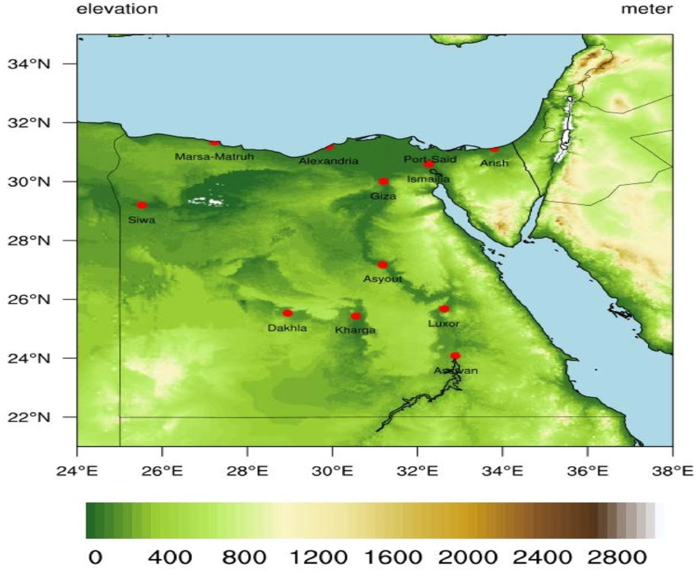
Figure 1. Surface elevation of Egypt (in meters). The red dots indicate the location of the ten locations for evaluating the RegCM’s performance concerning the climatological annual cycle.
Hydrology 11 00121 g001
Figure 2. Potential evapotranspiration over the period 1981–2010 (PET; in mm day−1) for the MAM season in the first row (af); JJA in the second (gl); SON in the third (mr); and DJF in the fourth (sx). For each row, BATS is on the left, followed by CLM45; ERA5 is the third from the left, BATS minus ERA5, CLM45 minus ERA5, and the difference between CLM45 and BATS. Significant difference/bias are indicated in black dots using Student’s t-test with alpha equal to 5%. ERA5 is the ERA5-land-based product (hPET).
Hydrology 11 00121 g002
Figure 3. Potential evapotranspiration over the period 1981–2010 (PET; in mm day−1) for the MAM season in the first row (af); JJA in the second (gl); SON in the third (mr); and DJF in the fourth (sx). For each row, HS is on the left, followed by HSnew; ERA5 is the third from the left, HS minus ERA5, HSnew minus ERA5 and the difference between HSnew and HS. Significant difference/bias are indicated in black dots using Student’s t-test with alpha equal to 5%. Note that HS stands for the Hargreaves and Samani equation before the calibration, while HSnew refers to the calibrated Hargreaves and Samani equation. ERA5 is the ERA5-land-based product (hPET).
Hydrology 11 00121 g003
Figure 4. Potential evapotranspiration over the period 1981–2010 (PET; in mm day−1) for MAM season in the first row (af); JJA in the second (gl); SON in the third (mr); and DJF in the fourth (sx). For each row, the HOLT is on the left, followed by the UW; ERA5 is the third from left, HOLT minus ERA5, UW minus ERA5, and the difference between the UW and HOLT. Significant difference/bias are indicated in black dots using Student’s t-test with alpha equal to 5%. ERA5 is the ERA5-land-based product (hPET).
Hydrology 11 00121 g004
Figure 5. Potential evapotranspiration over the period 1981–2010 (PET; in mm day−1) for the MAM season in the first row (af); JJA in the second (gl); SON in the third (mr); and DJF in the fourth (sx). For each row, the TEMP is on the left, followed by the RAD; ERA5 is the third from left, TEMP minus ERA5, RAD minus ERA5, and the difference between RAD and TEMP. Significant difference/bias are indicated in black dots using Student’s t-test with alpha equal to 5%. Note that TEMP refers to the temperature-only version of the Hargreaves and Samani equation, while RAD refers to the temperature-radiation version of the Hargreaves and Samani equation. ERA5 is the ERA5-land-based product (hPET).
Hydrology 11 00121 g005
Figure 6. Potential evapotranspiration over the evaluation period 1981–1996 (PET; in mm day−1) for the MAM season in the first row (af); JJA in the second (gl); SON in the third (mr); and DJF in the fourth (sx). For each row, the OLD is on the left, followed by the NEW; ERA5 is the third from the left, OLD minus ERA5, NEW minus ERA5, and the difference between NEW and OLD. Significant difference/bias are indicated in black dots using Student’s t-test with alpha equal to 5%. Note that OLD refers to the calibrated Hargreaves and Samani equation before applying the LS bias-correction method, while NEW refers to the calibrated Hargreaves and Samani equation after applying the LS bias-correction method. ERA5 is the ERA5-land-based product (hPET).
Hydrology 11 00121 g006
Figure 7. Potential evapotranspiration over the validation period 1997–2010 (PET; in mm day−1) for the MAM season in the first row (af); JJA in the second (gl); SON in the third (mr); and DJF in the fourth (sx). For each row, the OLD is on the left, followed by the NEW; ERA5 is the third from the left, OLD minus ERA5, NEW minus ERA5, and the difference between NEW and OLD. Significant difference/bias are indicated in black dots using Student’s t-test with alpha equal to 5%. Note that OLD refers to the calibrated Hargreaves and Samani equation before applying the LS bias-correction method, while NEW refers to the calibrated Hargreaves and Samani equation after applying the LS bias-correction method. ERA5 is the ERA5-land-based product (hPET).
Hydrology 11 00121 g007
Figure 8. Climatological annual cycle of the potential evapotranspiration over the period 1981–2010 (PET; in mm day−1) derived from the ERA5-land-based product (hPET) for the ten locations: Alexandria, Arish, Asswan, Asyout, Dakhla, Giza, Ismailia, Kharga, Luxor, and Siwa.
Hydrology 11 00121 g008
Figure 9. Climatological annual cycle of the simulated PET with respect to the ERA5 over the validation period 1997–2010 (for the locations indicated in Figure 1). Note that OLD (in blue) refers to the calibrated Hargreaves and Samani equation before applying the LS bias-correction method, while NEW (in red) refers to the calibrated Hargreaves and Samani equation after applying the LS bias-correction method. OBS is the ERA5-land-based product (hPET).
Hydrology 11 00121 g009
Figure 10. Taylor diagram to quantify the performance of the RegCM4 concerning the PET climatological annual cycle over the validation period 1997–2010 (for the locations indicated in Figure 1). Note that OLD (in red) refers to the calibrated Hargreaves and Samani equation before applying the LS bias-correction method, while NEW (in blue) refers to the calibrated Hargreaves and Samani equation after applying the LS bias-correction method.
Hydrology 11 00121 g010
Disclaimer/Publisher’s Note: The statements, opinions and data contained in all publications are solely those of the individual author(s) and contributor(s) and not of MDPI and/or the editor(s). MDPI and/or the editor(s) disclaim responsibility for any injury to people or property resulting from any ideas, methods, instructions or products referred to in the content.