Abstract
A univariate analysis that relies solely on precipitation data in low flow frequency analysis is a technique to express meteorological drought, so it is limited to analyzing the characteristics of hydrological drought related to available water resources. In addition, if the data for the model calibration are insufficient, the uncertainty of a single variable limits the construction of a reliable model. To improve this problem, a frequency analysis was performed by constructing a bivariate copula model as a multivariate model with a high correlation between variables targeting reservoir inflows. The methodology utilizes the theory of runs to identify low flow events, establishing a threshold based on the mandatory regional water supply plan, and determining the low flow duration and cumulative water deficit. The Gumbel copula function, effective in capturing correlations between hydrological variables, was applied to derive a joint bivariate probability distribution, facilitating the calculation of combined low flow event return periods. This study compared low flow frequencies at Soyanggang dam (’74–’22) and Chungju dam (’86–’22), which are in the same Han River basin but have different capacities and water demands, using a bivariate copula model. The top four extreme low flow events for the two adjacent dam basins did not occur in the same year and, in the years of the extreme low flow events at one of the two dam basins, there was an insignificant magnitude at the remaining dam basin. This result is noteworthy because it shows that the possibility of extreme low flow events appearing simultaneously in both watersheds is not as high as expected. The operational efficiency can be improved by setting the coordinated operation rules of the two reservoirs using the copula dependency structure.
1. Introduction
Drought, characterized by an extended period of abnormally low precipitation resulting in water scarcity, exerts significant impacts on agriculture, ecosystems, water resources, and society. Quantifying drought magnitude is essential for its analysis and frequency assessment. However, due to the ambiguity in delineating its onset and termination, various methodologies are possible to establish clear thresholds based on rainfall or river runoff. In the assessment of meteorological drought, researchers have pursued univariate low flow frequency analysis predicated on precipitation data [1,2,3]. Univariate low flow frequency analysis, utilizing precipitation as its primary variable, involves establishing a baseline precipitation level to ascertain both the duration and magnitude of the low flow event. Each of these parameters is treated as an independent variable in order to derive the frequency of low flow occurrences, referred to as the return period. While univariate analysis considers either the duration or magnitude of low flow independently, there is also a growing interest in multivariate low flow frequency analysis, which takes into account the dependency between the duration and the magnitude [4,5]. A univariate analysis that relies solely on precipitation data in low flow frequency analysis is a technique to express meteorological drought, so it is limited to analyzing the characteristics of hydrological drought related to available water resources. In addition, if the data for the model calibration are insufficient, the uncertainty of a single variable limits the construction of a reliable model. In order to improve this problem, a frequency analysis was performed by constructing a bivariate copula model as a multivariate model with a high correlation between variables targeting reservoir inflows. The multivariate copula model has been the subject of significant research attention, as evidenced by studies conducted by [6,7].
Particularly, research on multivariate frequency analysis has predominantly utilized the copula model, as evidenced by studies conducted by [1,2,3,8]. Within the framework of the copula model, the interrelation among various low flow factors in a low flow frequency analysis can be encapsulated and elucidated through the copula function. This enables the derivation of a combined return period that accounts for both the duration and severity of low flow events. The copula function serves to articulate the dependence structure and correlation among low flow components, which are crucial for estimating low flow frequency. Furthermore, it facilitates the analysis of the impact of multiple parameters, including uncertainty, in multivariate frequency analysis. Consequently, it becomes feasible to ascertain the frequency of low flow events that comprehensively encapsulates the influence of various low flow characteristics, in contrast to the conventional univariate frequency analysis method [8]. While meteorological models focusing on precipitation have historically dominated low flow analysis, there is a growing recognition of the necessity for hydrological low flow analysis targeting basin or river runoff. Such an analysis is imperative for assessing the decline in river and reservoir inflows, consequent reductions in dam water storage capacities, and the inadequacy of the water supply to meet demand.
In a hydrological investigation conducted by [9], a copula bivariate low flow frequency analysis was employed utilizing streamflow data. This approach enables a quantitative assessment of the low flow return period, facilitating the inference of low flow severity and duration corresponding to specific return periods, thereby allowing for the characterization of low flow tendencies. Notably, it is crucial to acknowledge that the outcomes of such an analysis can exhibit substantial variability contingent upon the threshold criteria applied to runoff measurements. For instance, if the average monthly outflow is designated as the threshold, and daily outflow is classified as indicative of low flow, the identified low flow events may diverge significantly from actual occurrences. Furthermore, ref. [10] conducted a study where the threshold was established based on water supply and the low flow return period was exclusively derived from low flow duration, highlighting a limitation wherein considerable uncertainty was observed, particularly regarding low flow conditions.
In this investigation, a bivariate low flow frequency analysis employing the copula model was conducted utilizing dam inflow data from both the Soyanggang dam and the Chungju dam. Initially, the onset and termination of low flow events were delineated utilizing the Theory of Runs proposed by [11]. To facilitate a quantitative interpretation of low flow occurrences, the mean of the monthly mandatory water supply served as the threshold level, enabling the derivation of characteristic low flow events. Low flow events were then subjected to bivariate analysis utilizing the copula model, which allows for the simultaneous consideration of multiple low flow characteristics. The evaluation of low flow events was further enhanced through the calculation of their return periods. Finally, the geographically adjacent two dam basins were compared with respect to the return periods and the resulting hydro-statistical homo- or heterogeneity, which could offer insights for establishing the coordinated operation rules applicable during low flow events.
2. Study Area and Data Sets
In this study, the Soyanggang dam and Chungju dam basins were chosen as the target areas for conducting low flow frequency analysis (see Figure 1). The Soyanggang dam, located in Chuncheon-si, Gangwon-do, is a rockfill dam recorded as the highest in Korea. It encompasses a total basin area of 2783.3 km2 and spans a flow path of 234.2 km. Conversely, the Chungju dam, located in Chungju-si, Chungcheongbuk-do, is a concrete gravity dam holding the largest storage capacity in Korea, covering a total basin area of 4257.2 km2 with a flow path of 261.2 km. For the duration of this study, daily inflow data during ’74–’22 from the Soyanggang dam and during ’86–’22 from the Chungju dam were utilized, spanning the months of February to October each year. These data were employed to assess the sensible extent of low flow based on water demand. The inflow data were sourced from the National Water Resources Management Comprehensive Information System (WAMIS http://www.wamis.go.kr/ accessed on 1 April 2024), managed by the Han River Flood Control Center. Upon preliminarily examining the data, it was observed that there was a notable number of freezing days causing missing data. Those seasonal missing or extreme low flow data were excluded from the analysis because they would result in underestimating the low flow return period. Additionally, there were no long-term missing values during the analysis period except for winter season, and missing values within 3 days were interpolated by averaging the daily data before and after the missing value standard. The basic statistics of the inflow data at two dam basins are summarized in the Table 1.
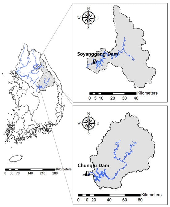
Figure 1.
Basin map for Soyanggang dam and Chungju dam.

Table 1.
Basic statistics of the dam inflows at Soyanggang and Chungju dam basins.
3. Methodology
Figure 2 illustrates a procedural flow chart delineating the steps involved in conducting copula low flow frequency analysis within the context of this study. (1) Initially, the Theory of Runs is utilized to establish the threshold level, duration of low flow, and cumulative water deficit (depth). (2) Subsequently, individual univariate probability distributions are computed based on the predetermined duration of low flow and cumulative water deficit. The return period is then determined using the non-exceedance probability associated with each univariate probability distribution. (3) The bivariate combined probability distribution is then computed by combining the previously obtained univariate probability distributions through the utilization of the copula function. Consequently, the combined return period is derived. Ultimately, the evaluation of low flow events is conducted by comparing the return period associated with each low flow duration and cumulative deficit, derived from univariate low flow frequency analysis, with the combined copula return period resulting from bivariate low flow frequency analysis.
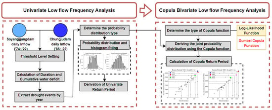
Figure 2.
Procedure for the copula low flow frequency analysis.
3.1. Theory of Runs
Before conducting low flow frequency analysis, it is essential to establish the onset and termination of low flow periods and quantify the magnitude of the low flow. The data available for this study comprised time-series data, which constitute a sequential set of observations over time. To compute the univariate probability distribution and conduct low flow frequency analysis utilizing the copula function, the parameters associated with the copula function derived from time-series data are necessary. The theory of runs, a statistical method, was introduced for delineating the initiation and termination of low flows and estimating their severity [11].
A “Run” denotes a continuous time-series segment featuring solely negative runs for values below the specified threshold level and positive runs for values exceeding the threshold level, observed between two consecutive intersection points. To calculate runs, parameters such as threshold, supply, demand, low flow intensity, low flow depth, and duration should be defined. Depending on the analysis objective, precipitation, runoff, surplus or deficit in supply, low flow indices, etc., can be used for defining the threshold in diverse manners. To interpret low flow frequency utilizing the theory of runs, it is imperative to select an appropriate threshold level, criteria for identifying extreme low flows, and to investigate and analyze the statistical and time-series characteristics of low flow events.
Unlike existing low flow frequency analysis using rainfall or river flow, in this study, a copula model was constructed for the inflow of multi-purpose dams. Consequently, the low flow duration was based on inflow utilizing the runs theory, and parameters such as duration and cumulative water deficit were determined. As depicted in Figure 3, the area below the threshold level was designated as the cumulative water deficit (SD), the duration (TD) was defined as the time between the onset and termination of the cumulative water deficit, and the threshold (X0) was established. In the drought analysis based on the run theory, the average daily flow rate expressed as m3/s was used as the raw data. A drought event was defined using a daily flow rate time series and a specific threshold, and the duration of an event usually lasted from several weeks to months (Figure 3b).
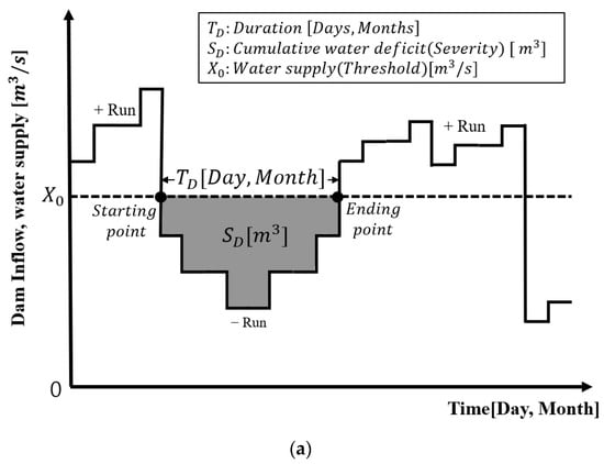
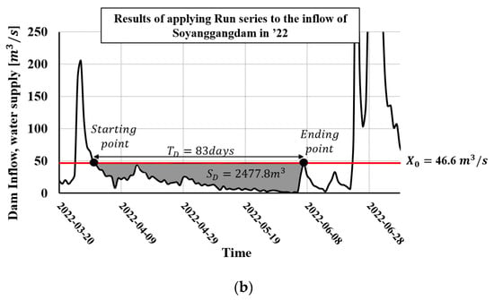
Figure 3.
Conceptual diagram of the runs theory and its actual application [11]. (a) Conceptual diagram. (b) Duration and cumulative water deficit in actual time-series data.
The mandatory water supply corresponds to the constant water supply volume pro-vided by the reservoir, accounting for inflow, storage, outflow, and demand. The water supply encompasses municipal, agricultural, and in-stream water requirements, with varying values for each month to accommodate seasonality. However, in this study, as events were derived annually and the return period was expressed in years, the mandatory water supply amount was utilized as the threshold for defining the low flow events from the entire inflow time series, which can be regarded as the deficit between the reservoir inflow and water supply from a reservoir.
3.2. Univariate Low Flow Frequency Analysis
To estimate the duration of low flow and the return period of cumulative deficit through univariate low flow frequency analysis, it is imperative to first calculate the univariate probability distribution. Additionally, since the copula model is a statistical framework that expresses the correlation between variables by deriving a joint probability distribution from the univariate probability distributions of individual variables, it is indispensable to compute the univariate probability distribution for both univariate and bivariate low flow frequency analyses.
Initially, the optimal probability distribution and parameters were determined through a goodness-of-fit test based on the maximum duration (in days) and cumulative water deficit (in cm) of daily inflow data from the Soyanggang dam (’74–’22) and Chungju dam (’86–’22). Subsequently, the probability distribution type was determined through the aforementioned test methods, and the univariate probability distribution was computed by applying it to both the duration and cumulative water deficit variables. Next, the return period was derived using the results of the univariate probability distribution for low flow duration and cumulative water deficit. Typically, univariate frequency analysis includes methods such as the probability plotting position method, which generates series with the highest values or exceedance series from hydrological data, and probability distribution tests employing probability paper. These methods aim to determine the return period of a hydrological event of a specific magnitude or the magnitude of a hydrological event during a specific return period. In this study, a methodology was employed to derive the return period for each duration and cumulative deficit using the non-exceedance probability (P = 1 − exceedance probability) derived from the univariate joint probability distribution based on the aforementioned methods. The return period is defined as a certain magnitude occurring more than once on average every T year and is expressed as the reciprocal of the probability of exceedance.
3.3. Bivariate Copula Low Flow Frequency Analysis
The copula model, introduced by Sklar (1959), has predominantly been employed in the finance sector to explain complex dependency structures [12]. Conventional low flow frequency analysis is typically grounded in the derivation and analysis of return periods based on univariate probability distributions for each duration and severity of low flow events. However, when examining low flow frequency, the copula function can serve as a valuable tool for establishing connections between individual univariate probability distributions, thereby facilitating the creation of a joint probability distribution to uncover correlations between variables that may not be discernible from the univariate probability distributions alone. In the context of this study, the copula model is represented by Equation (1), which pertains to scenarios involving two random variables X and Y, and encompasses a joint distribution function C linking the two variables. Herein, the joint probability distribution is expressed as a function of FX(x), FY(y).
Copula models are categorized into two main types: Elliptical copula and Archimedean copula. While Elliptical copula has an advantage of being represented as a multi-dimensional distribution, it is noted that its parameter estimation can be complex, especially for high-dimensional data or when dealing with non-standard copula families. Therefore, careful attention should be paid to the assumptions underlying the chosen model and the validity of the estimation procedure. Hence, in the context of low flow frequency analysis, the Archimedean copula is often preferred due to its ability to effectively capture correlations between hydrological variables [2]. Common types of Archimedean copula functions utilized in copula frequency analysis include Clayton copula, Frank copula, and Gumbel copula [13,14]. The choice of the distribution function is made based on the symmetricity of the observed data considering the shape parameters, e.g., skewness and kurtosis. However, if the size of the dataset is not sufficient, the determination of the probability distribution should not depend solely on the shape parameter and is bound to involve empirical judgment.
The Clayton copula is characterized by enhancing the dependency of the left tail structure in the probability distribution, thereby modeling strong correlation between variables in the left tail. This function is suitable for scenarios where one region’s rainfall tends to correlate with rainfall in a non-adjacent region, indicating low correlation between the two variables. The Frank copula is favored for identifying correlations between two variables exhibiting both negative and positive correlations. It is well-suited for examining trends across a broad range of data. For instance, it is useful when analyzing how the average and extreme values of rainfall variables in distinct regions correlate differently. Lastly, the Gumbel copula is effective for modeling the tail of a symmetrical probability distribution, particularly for extreme values exhibiting positive correlation. This function is commonly applied in hydrological research to understand the behavior of variables associated with extreme events, such as extreme floods and droughts. The types and parameter ranges of Archimedean copula functions are summarized in Table 2 [15].

Table 2.
Types of copula functions.
The canonical maximum likelihood method (CML) was used to determine the copula parameter, θc. CML is a method of estimating the copula parameter using the parameters of each distribution function by converting individual data into a uniform distribution. After deriving the probability distribution function of the cumulative deficit, denoted as FX(x), FY(y), and determining the suitable copula function, the joint distribution probability is calculated using the corresponding copula function to ascertain the bivariate low flow return period. This calculation considers both the duration of the low flow and the cumulative deficit concurrently. Specifically, when both conditions that ① the duration exceeds a certain threshold and ② the cumulative deficit surpasses a specific value are met simultaneously, Equation (2) is applied. Conversely, when only one of the conditions is satisfied, the scenario is expressed using Equation (3). Here, TDS represents the joint return period when both the duration and the cumulative deficit exceed their specific thresholds.
4. Application and Results
In this study, the threshold for low flow assessment was established as the average annual planning water supply for both Soyanggang dam and Chungju dam. The average annual mandatory water supplies are 46.6 m3/s for Soyanggang dam and 107.2 m3/s for Chungju dam, respectively. Utilizing the runs theory outlined in Section 3.1, the maximum annual events for both dams were computed based on the thresholds set for duration and cumulative deficit, as illustrated in columns 2, 3, 6, and 7 of Table 6. Before bivariate copula model calibration, the univariate model calibration should be performed. The goodness-of-fit test for univariate data assesses how well the data align with the theoretical distribution or expected value and typically employs validation methods such as the Chi-squared test, Kolmogorov–Smirnov test, and Anderson–Darling test [16]. However, the normal distribution was adopted as the probability distribution of the two parameters through the empirical intuition based on the assumption that there are insufficient reasons that the low flow variables are unsymmetrically skewed as explained in the following.
To compute the univariate probability distribution, the variables for duration and cumulative deficit at both dams were partitioned into equal intervals, and a histogram was plotted (Figure 4). Upon examination of the histogram, it was observed that the frequency exhibited a symmetrical structure as a whole. The interval with peak frequency did not appear clearly but tended to be concentrated at the center of the distribution. This characteristic is indicative of a normal distribution, and measures of skewness and kurtosis were calculated to objectively assess the data’s suitability for normal distribution. An ideal normal distribution is indicated when the skewness equals 0 and the kurtosis equals 3. In general, for a normal distribution, the skewness should not exceed an absolute value of 3, and the kurtosis should not exceed an absolute value of 10. The skewness and kurtosis values for the data under consideration are presented in Table 3. Based on the results, it was determined that the skewness of all datasets fell within an absolute value of 3, and the kurtosis fell within an absolute value of 10. Consequently, the probability distribution for all copula variables was assumed to follow a normal distribution. The normal distribution referred to in the following sentence is a probability distribution known as the standard error curve when the sample size approaches infinity. The histogram and the derived normal distribution function curves are depicted in Figure 4a–d. The histogram was generated by dividing the data into eight equal-sized intervals.
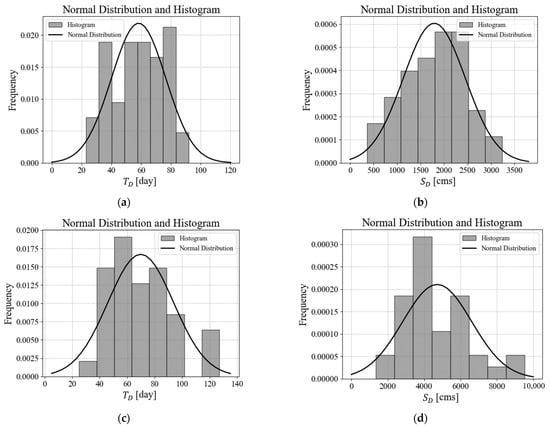
Figure 4.
The derived normal distribution and the histogram. (a) Duration for the Soyanggang dam. (b) Cumulative water deficit for the Soyanggang dam. (c) Duration for the Chungju dam. (d) Cumulative water deficit of the Chungju dam.

Table 3.
Skewness and kurtosis of the derived distribution for Soyanggang and Chungju dams.
To determine the univariate probability distribution as a normal distribution and calculate the bivariate return period, the sum of the copula joint probability distributions must be the same as the marginal probability distribution. The joint probability distribution refers to the cumulative probability distribution of two random variables X and Y defined in the sample space S, and it is expressed as Equation (4).
The copula function is an effective technique for analyzing whether the variables to be analyzed are correlated with interdependence. Therefore, the correlation coefficients between the durations and cumulative deficits of Soyanggang dam and Chungju dam were calculated to test whether there was a correlation between variables before applying the copula function. The correlation coefficient values between the duration and the cumulative deficit were 0.9584 for Soyanggang dam and 0.9796 for Chungju dam, respectively, indicating that both dams had a positive correlation between the duration and the cumulative deficit. As mentioned in Section 3, the Clayton copula is suitable when there is a high correlation between the left tail of the data distribution, the Frank copula is suitable when the correlation between the right tail data is high, and the Gumbel copula is a suitable copula function when the correlation between both tails of the data is high. Referring to Figure 5, it was judged that the duration and cumulative water deficit data distribution of Soyanggang dam and Chungju dam were very highly correlated in all ranges, including the right and left tail structure. From this, it can be inferred that it was appropriate to use the Gumbel copula among the Clayton, Frank, and Gumbel copulas.
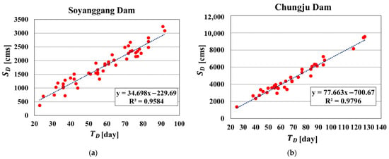
Figure 5.
Correlation between duration and cumulative water deficit for Soyanggang and Chungju dams. (a) Soyanggang dam. (b) Chungju dam.
Based on the correlation analysis, the logarithmic likelihood function was used as mentioned in Section 3.3 to determine whether the Gumbel copula function could be set as a joint distribution function. As for the logarithmic likelihood function, a copula function with a large value was selected as the optimal function as an index to determine the feasibility of the copula function [17]. The following is a table showing the results of applying the logarithmic likelihood function (Table 4).

Table 4.
Estimation of log-likelihood function for Soyanggang and Chungju dams.
As for the log-likelihood function value, the Gumbel copula function was the most feasible function for both Soyanggang and Chungju dams, and the results of calculating the Gumbel copula parameter through the estimated normal distribution parameter and log-likelihood function are suggested in Table 5.

Table 5.
Gumbel copula parameters for Soyanggang and Chungju dams.
Based on the application of the Gumbel copula for calculating return periods, the most severe low flow at the Soyanggang dam occurred in 1996, characterized by a duration of 91 days, a cumulative deficit of 3237.8 m3/s, and a copula return period of 69.6 years (Table 6). Subsequent notable events included copula return periods of 39.6 years in 1979, 17.1 years in 2008, and 11.8 years in 1982. The average dam inflow in 1996 and 1995 was 59.6 and 125.0 m3/s, respectively, indicating a decrease of approximately 47% in the dam inflow in 1996 compared to the previous year. Notably, during the flood season of the same year, the daily inflow increased by up to 1279.5 m3/s, and this was attributed to significantly increased rainfall. However, a comprehensive evaluation of the water supply safety index, comprising the dam inflow, dam water supply, and water deficit, concluded that a water supply failure did not occur at Soyanggang dam in 1996. Similarly, in 1979, the second most severe year after 1996, there was no significant water supply failure, with non-flood season inflows not markedly different from the previous year, 1978, although the flood season inflow increased to 392.8 m3/s. Furthermore, an analysis of rainfall in Gangwon-do in 2008, during the record high low flow, revealed that only 63% of the average monthly rainfall occurred, dropping to approximately 45% in October at the onset of the dry season.

Table 6.
Summary of low flow events and associated copula return periods.
In this analysis, the four most extreme low flow events for each dam were selected and the copula return periods were compared with univariate return periods between two dam basins (Figure 6, Table 7). Initially, when employing the normal distribution to compute return periods for individual durations and cumulative deficits, substantial deviations in ranking were observed. Similarly, when applying the Gumbel copula function to calculate the joint return periods, significant deviations in ranking persisted. The normal distribution probability and copula joint probability calculated in this study exhibited lower statistical estimation errors, offering more reliable results as the dataset expanded for statistical analysis. However, due to the ambiguity in delineating its onset and termination, various methodologies are possible to establish clear thresholds based on rainfall or river runoff. In the assessment of meteorological drought, researchers have pursued univariate low flow frequency analysis predicated on precipitation data [1,2,3]. Both dams showed that the copula return periods were closer to the univariate return periods for severity rather than duration. The top four extreme low flow events in Soyanggang dam basin were observed in 1996, 1979, 2008, and 1982, giving 69.6, 39.6, 17.1, and 11.8, respectively. The years of the top four extreme events between the two dam basins were completely different. The top four extreme low flow events in Chungju dam basin were observed in 1989, 1988, 2000, and 2014, giving 180.1, 156.0, 45.6 and 11.0, respectively.
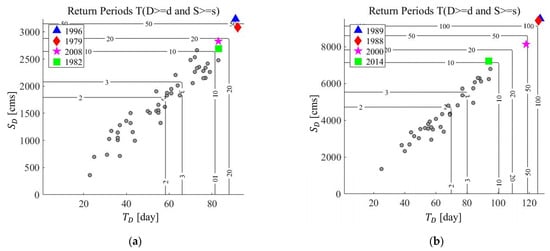
Figure 6.
SDF curves for the Soyanggang and Chungju dam basins. (a) Soyanggang dam. (b) Chungju dam.

Table 7.
Results of the top 4 return periods for each dam basin.
5. Conclusions
In order to quantify and evaluate hydrological drought, the return period of low flow that occurred in the target watershed in the past was derived through copula frequency analysis using inflow data from Soyanggang dam (’74–’22) and Chungju dam (’86–’22) in this study. The low flow occurrence event was extracted by defining the onset and termination of the low flow period using the theory of runs, calculating the size of the low flow that occurred during this period, and setting the duration and cumulative deficit as variables. The two defined variables (duration, cumulative deficit) were set as parameters for copula bivariate frequency analysis. A normal distribution was adopted as the probability distribution of the two parameters through empirical intuition based on the assumption that there were insufficient reasons that the low flow variables were unsymmetrically skewed. In addition, the Gumbel copula function was adopted as a result of calculating using the logarithmic likelihood function to determine the appropriate copula function for the data used in this study, and the Gumbel copula parameter was calculated. Then, based on the calculated parameters, the Gumbel copula return periods of the annual low flow event of Soyanggang and Chungju dams were calculated.
In this study, a bivariate low flow frequency analysis was performed using the copula function, and two independent variables were used to express a low flow that could not be quantitatively defined as a single return period to define the characteristics of low flow. Through the low flow frequency analysis using the copula function based on the inflow of dams, it was possible to confirm the duration of insufficient inflows corresponding to the extreme low flow years of the Soyanggang and Chungju dams, and the corresponding inflows were possible to determine the quantitative low flow frequency by deriving the copula return period. Based on the results of the copula frequency analysis, it was possible to confirm the lack of precipitation, the inflow of low flow rates, and the decrease in the water reserve rates, which are the causes of the hydrological low flow that occurred in the low flow year.
Soyanggang dam and Chungju dam are both located within the same Han River basin and are geographically close to each other, but the size of the reservoir, basin area, and water supply capacity are different, so the low flow characteristics may appear very different despite being under similar weather conditions. In addition, low flow events are different from flood events, and any protocol is rarely found for calculating the frequency (or return period) of low flow events that can be used for planning and (/or) operation of water resources facilities. This means that the planning of water resource facilities to prepare for low flow, water shortage events, or the low flow management criteria for water supply in case of a low flow inevitably depend on the operator’s subjective judgment. A low flow frequency analysis for dam operation can provide a more realistic criterion for determining the dam operator when set based on the amount of dam inflow observation.
Most of the low flow frequency analysis conducted in Korea until recently was based on rainfall. However, in this study, the frequency analysis was performed based on the inflow of the Soyanggang and Chungju dams. As a result, the top four most extreme low flow events were in 1996, 1979, 2008, and 1982 at Soyanggang dam basin, whereas the Chungju dam showed somewhat different years for the top extreme events in 1989, 1988, 2000, and 2014. The return periods of the top four years were 69.6, 39.6, 17.1, 11.8 years for Soyanggang dam basin, and 180.1, 156.0, 45.6, and 10.7 years for Chungju dam basin, indicating that the magnitudes of the low flow events of Chungju dam were somewhat greater. Since none of the top four low flow events of the two dams occurred in the same year, the low flow frequency for eight years was compared. Among the top four events of Soyanggang dam, the low flow return periods of Chungju dam in 1996 and 2008, except for 1979 and 1982, were 4.7 and 6.4 years, respectively, which were quite small compared to 69.6 and 17.1 years for Soyanggang dam. On the other hand, the low flow return periods of Soyanggang dam in the years corresponding to the top four disasters of Chungju Dam (1989, 1988, 2000, and 2014) were 1.1, 6.7, 8.0, and 7.6 years, respectively, which were very small compared to the 180.1, 156.0, 45.6, and 10.7 years for Chungju dam. This result is noteworthy because while high-frequency (low return period) low flow events may have had a high correlation between the two basins, the correlation in low-frequency (high reproduction period) low flow events with high magnitude was not high.
In general, it is estimated that meteorological correlations will be high in geographically adjacent basins, but hydrological correlations may not be very high. In other words, it means that the possibility of extreme low flow events appearing simultaneously in both watersheds is not as high as expected, suggesting that the effect of the coordinated operation of the two reservoirs may be high. If this fact can be more clearly proved through the accumulated data in the future, it means that operational efficiency can be improved by setting the coordinated operation rules of the two reservoirs using it. In addition, based on the evaluation of extreme low flow years and water demand based on inflows conducted in this study, it can be taken as a signal that the long-term management and planning of Soyanggang dam and Chungju dam due to temporary or climate change are necessary.
Author Contributions
Conceptualization, J.S. and B.K.; methodology, J.S. and B.K.; validation, J.S. and B.K.; formal analysis, J.S.; data curation, J.S.; writing—original draft preparation, J.S. and B.K.; writing—review and editing, J.S. and B.K.; visualization, J.S.; supervision, B.K.; project administration, B.K.; funding acquisition, B.K. All authors have read and agreed to the published version of the manuscript.
Funding
The present research was supported by the research fund of Dankook university in 2021 (Grant #: R202101255).
Data Availability Statement
The data used for this study are available in the Korean Water Resources Management Information System (WAMIS) at http://www.wamis.go.kr/ accessed on1 April 2024.
Conflicts of Interest
The authors declare no conflicts of interest. The funders had no role in the design of the study; in the collection, analyses, or interpretation of data; in the writing of the manuscript; or in the decision to publish the results.
References
- Yoo, J.Y.; Shin, J.Y.; Kim, D.; Kim, T.W. Drought risk analysis using stochastic rainfall generation model and copula functions. J. Korea Water Resour. Assoc. 2013, 46, 425–437. [Google Scholar] [CrossRef]
- Yoo, J.; Kim, D.; Kim, H.; Kim, T.W. Application of copula functions to construct confidence intervals of bivariate drought frequency curve. J. Hydro-Environ. Res. 2016, 11, 113–122. [Google Scholar] [CrossRef]
- Kim, J.-Y.; So, B.-J.; Kim, T.-W.; Kwon, H.-H. A development of trivariate drought frequency analysis approach using copula function. J. Korea Water Resour. Assoc. 2016, 49, 823–833. [Google Scholar]
- Zhang, L.; Singh, V.P. Bivariate flood frequency analysis using the copula method. J. Hydrol. Eng. 2006, 11, 150–164. [Google Scholar] [CrossRef]
- González, J.; Valdés, J.B. Bivariate drought recurrence analysis using tree ring reconstructions. J. Hydrol. Eng. 2003, 8, 247–258. [Google Scholar] [CrossRef]
- Bayazit, M.; Fernandez, B.; Salas, J. Return Period and Risk of Hydrologic Events. I: Mathematical Formulation. J. Hydrol. Eng. 2001, 6, 358–363. [Google Scholar] [CrossRef]
- Son, K.-H.; Bae, D.-H.; Chung, J.-S. Drought Analysis and Assessment by Using Land Surface Model on South Korea. J. Korea Water Resour. Assoc. 2011, 44, 667–681. [Google Scholar] [CrossRef]
- Van deVyver, H.; Van den Bergh, J. The Gaussian copula model for the joint deficit index for droughts. J. Hydrol. 2018, 561, 987–999. [Google Scholar] [CrossRef]
- Kwak, J.W.; Kim, D.G.; Lee, J.S.; Kim, H.S. Hydrological Drought Analysis using Copula Theory. KSCE J. Civ. Environ. Eng. Res. 2012, 32, 161–168. [Google Scholar] [CrossRef]
- Sung, J.H.; Chung, E.-S. Application of Streamflow Drought Index using Threshold Level Method. J. Korea Water Resour. Assoc. 2014, 47, 491–500. [Google Scholar] [CrossRef]
- Yevjevich, V.M. Objective Approach to Definitions and Investigations of Continental Hydrologic Droughts; Hydrology Paper 23; Colorado State University: Fort Collins, CO, USA, 1967. [Google Scholar]
- Lee, G.H.; Lee, M.H.; Lee, J.H. Measuring the Systemic Risk in the Korean Banking Sector: The Copula Approach. J. Money Financ. 2013, 27, 81–123. [Google Scholar] [CrossRef]
- Haugh, M. An Introduction to Copulas: Quantitative Risk Management; Springer Science & Business Media: Berlin/Heidelberg, Germany, 2016. [Google Scholar]
- Boateng, M.A.; Omari-Sasu, A.Y.; Avuglah, R.K.; Frempong, N.K. A Mixture of Clayton, Gumbel, and Frank Copulas: A Complete Dependence Model. J. Probab. Stat. 2022, 1422394. [Google Scholar] [CrossRef]
- Nelssen, R.B. An Introduction to Copula; Springer: New York, NY, USA, 2006; pp. 109–115. [Google Scholar]
- Ang, A.H.-S.; Tang, W.H. Probability Concepts in Engineering: Emphasis on Applications in Civil & Environmental Engineering, 2nd ed.; Alfredo, H.-S., Ed.; John Wiley & Sons Inc.: Califonia, CA, USA, 2007. [Google Scholar]
- Ju, G.-W.; Shin, J.-Y.; Heo, J.-H. Bivariate Frequency Analysis of Rainfall using Copula Model. J. Korea Water Resour. Assoc. 2012, 45, 827–837. [Google Scholar] [CrossRef]
Disclaimer/Publisher’s Note: The statements, opinions and data contained in all publications are solely those of the individual author(s) and contributor(s) and not of MDPI and/or the editor(s). MDPI and/or the editor(s) disclaim responsibility for any injury to people or property resulting from any ideas, methods, instructions or products referred to in the content. |
© 2024 by the authors. Licensee MDPI, Basel, Switzerland. This article is an open access article distributed under the terms and conditions of the Creative Commons Attribution (CC BY) license (https://creativecommons.org/licenses/by/4.0/).